

Evaluation of Tree-Growth Rate in the Laurentides Wildlife Reserve Using GEDI and Airborne-LiDAR Data

Jet Propulsion Laboratory, California Institute of Technology, Pasadena, CA 91109, USA
*
Author to whom correspondence should be addressed.
Remote Sens. 2023, 15(22), 5352; https://doi.org/10.3390/rs15225352
Submission received: 6 October 2023
/
Revised: 10 November 2023
/
Accepted: 13 November 2023
/
Published: 14 November 2023
(This article belongs to the Special Issue Lidar for Environmental Remote Sensing: Theory and Application)
Abstract
:Loss of forest cover and derived effects on forest ecosystems services has led to the establishment of land management policies and forest monitoring systems, and consequently to the demand for accurate and multitemporal data on forest extent and structure. In recent years, spaceborne Light Detection and Ranging (LiDAR) missions, such as the Global Ecosystem Dynamics Investigation (GEDI) instrument, have facilitated the repeated acquisition of data on the vertical structure of vegetation. In this study, we designed an approach incorporating GEDI and airborne LiDAR data, in addition to detailed forestry inventory data, for estimating tree-growth dynamics for the Laurentides wildlife reserve in Canada. We estimated an average tree-growth rate of 0.32 ± 0.23 (SD) m/year for the study site and evaluated our results against field data and a time series of NDVI from Landsat images. The results are in agreement with expected patterns in tree-growth rates related to tree species and forest stand age, and the produced dataset is able to track disturbance events resulting in the loss of canopy height. Our study demonstrates the benefits of using spaceborne-LiDAR data for extending the temporal coverage of forestry inventories and highlights the ability of GEDI data for detecting changes in forests’ vertical structure.
1. Introduction
Establishing forest monitoring systems has become an important objective of international agencies and national governments due to concerns over current deforestation rates and derived loss of forest ecosystem services [1,2]. In particular, forests’ function as sinks of carbon emissions has become a focal point for strategies of climate change mitigation, and different countries have adopted policies for enhancing carbon storage in forests via afforestation and reforestation in accordance with Global climate agreements and environmental conventions [3,4,5]. Programs such as reducing emissions from deforestation and forest degradation (REDD+) rely on the estimation of baselines of carbon stocks in forests and on carbon stock change detection to evaluate the achievement of goals and determine result-based payments [6,7,8]. The implementation of these land management policies and monitoring systems has resulted in the need to produce accurate and multitemporal data on forest extent and structure [9].
As part of the assessment of forest condition, the estimation of tree-growth rates is essential for understanding forest regeneration capacity after disturbance events [10] and carbon sequestration potential [11]. Furthermore, spatially explicit quantification of tree-growth dynamics is important for designing forest management strategies and estimating sustainable harvest levels [12], as well as for identifying climate change-related alterations on forest productivity [11,12,13].
Remote sensing technologies have become fundamental in the implementation of forest monitoring initiatives, due to their coverage of large areas, long-term monitoring capabilities, and the information on vegetation structure they produce [9,14,15]. For these reasons, and in contrast to ground inventories, remote sensing data are considered a cost- and time-effective solution for obtaining information over large or remote forested areas and for multitemporal-change detection [16]. Passive multispectral satellite imagery is widely used in forest monitoring systems, such as the Global Forest Watch [17], due to its capacity to acquire data over regular intervals, and the large repository of data available, particularly for Landsat imagery which spans several decades [18]. However, passive sensors are limited by cloud cover, and spectral signal saturation, especially in dense forests, that limits the estimation of some vegetation parameters such as tree-canopy height [19]. More recently, radar imagery has become commonly used in monitoring forested areas as this active remote sensing technology is less constrained by weather conditions [20,21,22]. Particularly, Interferometric Synthetic Aperture Radar (InSAR) is considered an efficient technique for estimating tree height [23,24,25,26]. Still, InSAR datasets for large-scale mapping and monitoring are not yet readily available in public repositories [20,27].
In contrast to optical and radar imagery, light detection and ranging (LiDAR) technology produces accurate data on the vertical forest structure at both regional and global scales [28,29,30,31,32]. However, despite its benefits in accuracy, data collection with airborne LiDAR systems can be cost prohibitive for large areas and for multitemporal acquisitions [33]. An alternative to producing repeated LiDAR acquisitions is spaceborne missions. NASA’s Global Ecosystems Dynamics Investigation (GEDI) instrument, launched to the International Space Station in 2018, has been successfully used to track changes in forest vertical structure, improving on the temporal coverage of global forest datasets [34,35,36]. GEDI is specifically designed to map ecosystem structure by using a full waveform LiDAR system with a nominal footprint size of ~25 m diameter that acquires information on the vertical structure of vegetation [37]. Moreover, GEDI data are publicly available with different levels of processing, which facilitates their use in various forestry applications [37]. In this study, we evaluate the benefits of using spaceborne and airborne LiDAR data in addition to forestry field measurements to track multitemporal changes in forest canopy height (i.e., tree growth) for a forest reserve in Canada. This study is in support of the Surface Topography and Vegetation, a Target Observable identified for maturation by the U.S. National Academies’ Decadal Survey [38].
2. Materials and Methods
We used the information from a forestry inventory containing airborne LiDAR and in situ data to determine the baseline conditions of a forested area, and the repeated acquisitions of GEDI to track changes in forest height beyond the initial acquisition date of the forestry inventory. As part of our approach, we first evaluate the accuracy of the GEDI Relative Height (RH) metrics compared to the airborne LiDAR data, then, we estimate average tree height growth at the forest stand level using GEDI height estimates, with airborne LiDAR estimates as a baseline. We evaluate our canopy growth results against the in situ forestry data and Landsat imagery.
2.1. Study Area and Input Data
Our study area was the Laurentides Wildlife Reserve (Réserve faunique des Laurentides), located 100 km north of Québec city, Canada. The reserve extends for 8900 km2 and is dominated by boreal and temperate forest cover and sustains an important ecotourism industry [39]. Intense forestry exploitation during the 20th century significantly reduced mature forest stands in the reserve, which, in addition to natural perturbations such as insect outbreaks, windthrow, and fires, has resulted in a heterogeneous landscape [39]. The differences in forest stand development makes the Laurentides reserve an interesting study area for assessing changes in canopy height due to different types of disturbances.
The Laurentides reserve has detailed field data available and complete coverage of airborne LiDAR data as part of the forestry inventories produced by the Québec government: “Inventaire Écoforestiere de Quebec Meridionel” [40]. Currently, there are five forestry inventories publicly available for the reserve. For our analysis we used the field data from permanent sample plots, the airborne-LiDAR raster products, and the forest stand classification defined in the inventory. All the information of the forestry inventory, as well as its documentation and user guides, were downloaded from the Québec government data portal: https://www.donneesquebec.ca/ (accessed on 12 July 2022).
The field data of the forestry inventory includes values of dbh, height, and species for individual trees located in permanent sample plots covering a large portion of the study area (Figure 1). The data from the permanent sample plots include a total of 3758 individual trees with available measurements for more than one survey date. This dataset was used for calculating rates of tree growth using the repeated measurements.
The airborne LiDAR data covering the Laurentides reserve were acquired over a total of five years, including 2013, 2015, 2016, 2017, and 2019 (Figure 1), and they are publicly available as processed products of Canopy Height Model (CHM), Digital Elevation Model (DEM) of 1 m pixel resolution, and a Slope product of 2 m pixel resolution. We used all three raster products in the analysis to determine the baseline conditions of the forest and to evaluate the terrain conditions of the study area.
The forest stand classification defined in the inventory was produced based on photointerpretation and expert knowledge of the area [40]. In this classification, each individual forest stand polygon indicates a group of trees relatively homogeneous in age, structure, composition, and environmental conditions [41]. The shapefile with the forest stand classification was processed following the forestry inventory documentation [40] to include information on type and year of disturbances.
We based the evaluation of tree growth with the forest stand as the unit of analysis and used the forest stand classification shapefile as the base layer of our workflow. The main assumption of our study was that the canopy height of individual trees in a specific forest stand is homogeneous and the average tree height within a stand represents the height of the trees in that polygon. Following this assumption, the sparse coverage of the GEDI data, which have a large separation between footprints, should still produce a good representation of the average tree height conditions of the forest stand.
All the available GEDI satellite passes covering the study area for dates between the years 2019 and 2022, inclusively, were downloaded and the relative height metrics of the L2A product “Elevation and Height Metrics Data”, and the canopy cover values of the L2B product “Canopy Cover and Vertical Profile Metrics data” were incorporated into the analysis. The dataset is available at the NASA/USGS Land Processes Distributed Active Archive Center [37].
![Remotesensing 15 05352 g001]()
Figure 1.
Study area and input data: (a) location of the Laurentides Wildlife reserve and its land-cover classification according to the Copernicus Global Land Service land cover map for 2019 [42]; (b) CHM product in meters; (c) coverage of the GEDI data available for the study area; (d) acquisition year of the airborne LiDAR data, with the coverage of each airborne acquisition represented in a different color; (e) location of the field-data permanent sample plots from the forestry inventory.

2.2. Data Preprocessing
We produced two accuracy assessments of the GEDI data against the CHM product, one at the footprint level, and another at the forest stand level. The objective of the assessment at the footprint level was to determine the best filtering process for the GEDI data, while the goal for the second assessment was to identify the aggregated GEDI RH metric that best represented the average-canopy-height condition for each forest stand. For these analyses, we assumed that the CHM product accurately represented the canopy-height conditions of the study area. Although airborne-LiDAR data are not exempt from biases and errors [43], there is agreement in the literature regarding the high accuracy of this data source [44,45]. For both analyses, only the overlapping airborne-LiDAR and GEDI data from the year 2019 were used as input, as this was the only concurrent acquisition date for the two datasets, which corresponded to a total of 130,374 GEDI footprints and to 2369 forests stands.
For the accuracy assessment at the footprint level, the GEDI data were filtered, following the products’ guides, by using the quality and degraded flags to filter out GEDI footprints with degraded or invalid measurements. Additionally, we removed footprints with zero detected modes, and filtered out any footprint that had a difference between the elevation of the highest return and the TanDEM-X value (included in the GEDI product) below or over 20 m. Considering that the GEDI data have a footprint of ~25 m in diameter, we processed the GEDI dataset as polygons instead of points, and evaluated the correspondence of the different RH metrics with the information from the CHM for each GEDI footprint.
For each GEDI footprint we first extracted the data from the CHM pixels within the footprint polygon and calculated different percentile values of canopy height. Using this approach, we evaluated how the GEDI RH metrics are related to the vertical structure detected by the airborne-LiDAR data. The correspondence between the GEDI RH metrics and the CHM percentiles was evaluated by visual assessment of the plotted data, and by calculating the Root Mean Squared Error (RMSE), Mean Absolute Error (MAE), bias, and Pearson’s correlation coefficient (CORR). The GEDI RH values 50, 70, 75, 80, 85, 88, 90, 95, 99, and 100, were evaluated against the CHM percentiles 30, 35, 40, 45, 50, 55, 60, 65, 70, 75, 80, 85, 88, 90, 95, and 100. After identifying the GEDI RH metric and CHM percentile with the best agreement, we analyzed the error distribution due to different parameters to determine the best filtering process for the GEDI data. The following parameters were considered: beam type, slope, elevation, tree cover (from the GEDI L2B product), Landsat tree cover, number of modes of the waveform, local and total energy of the return, solar elevation, acquisition date of the GEDI data, Landsat water permanence, and latitude. We used the performance statistics (CORR, RMSE, MAE, bias) in addition to the visual assessment of the plotted data to evaluate if a specific filtering process improved the correspondence of the datasets. Following this accuracy assessment analysis, the complete filtering processes for the GEDI data was established to include the parameters and thresholds listed in Table 1. The complete filtering process resulted in a final dataset of 688,249 GEDI footprints covering the study area, with a significant portion in the year 2020 (255,011 footprints).
For the second accuracy assessment, we aggregated the filtered GEDI data to the forest stand level by selecting only the GEDI points that were at least 11.2 m from the border of any forest stand. This threshold was determined so that approximately 90% of the GEDI footprint was inside a specific forest stand and the relative height information from the GEDI point was representative of the tree height within the forest stand. Using the GEDI points that overlapped each forest stand polygon, we calculated the mean, minimum, maximum, and standard deviation values of different RH metrics (85, 88, 90, 95, 99, 100) of the GEDI points grouped by acquisition year (2019, 2020, 2021, and 2022). Additionally, we calculated the number of GEDI footprints per forest stand and the point density, i.e., the number of GEDI points divided by the forest stand area; this last parameter was used for establishing whether a specific forest stand had sufficient GEDI data to be included in the tree-growth analysis. A minimum density threshold of 40 points per km2 was estimated by calculating an idealized circular GEDI-footprint coverage area of 145 m of diameter, or 0.0165 km2 (~25 m diameter of the footprint plus the 60 m along track separation between footprints, on each side of the footprint). We wanted to make sure that at least two thirds of the area of each forest stand were covered by GEDI points, which would result in a minimum ratio of one GEDI point per forest stand with an area of 0.025 km2.
The CHM, DEM, and terrain slope rasters were also aggregated by forest stand by calculating the mean and standard deviation values of all pixels overlapping each forest stand polygon. Finally, we evaluated the correspondence between the aggregated values of CHM and GEDI RH by visual assessment of the plotted data and by using the performance statistics (CORR, RMSE, MAE, bias). Following our assumption of tree-height homogeneity within each forest stand, our goal was to identify the aggregated GEDI RH metric that best represented the average-canopy-height condition, and then use this metric and the average CHM value to calculate tree growth. Therefore, we specifically focused on identifying the aggregated GEDI RH metric with the best fit against the mean CHM value.
2.3. Tree-Growth Estimation
For this study, tree growth was evaluated as the rate of change in average canopy height per forest stand. First, we filtered out forest stand polygons with an annual GEDI point density below 40 points/km2, then we constructed a time series of forest stand-height values using the average-CHM data, and the annual GEDI stand height estimates. The year range of the time series for each forest stand varied depending on the acquisition year of the airborne-LiDAR data (Figure 1d). Due to limitations in data availability, the resulting time series were not filtered by any specific year range; therefore, the shortest time difference between the GEDI and CHM data was one year, and the longest was nine years. Finally, we calculated the Theil–Sen slope [46,47] for each forest stand with the available data. The Theil–Sen slope analysis was selected due to its robustness to outliers, and for its higher efficiency for small datasets [46,48,49].
To calculate the statistics of tree growth in the Laurentides reserve, only forest stands with Theil–Sen slope values between 0 and 1 m/year were considered. The selection of these cut-off values aimed to improve the representation of actual tree-growth rates in the analysis dataset by removing values that were unlikely to correspond to real gains in canopy height, thus improving the quality of the data. Positive slope values beyond 1 m/year were likely not related to actual biological rates of gain in tree height, particularly considering that trees in the boreal forest grow at a rate of up to 1 m per year [50]. Furthermore, negative slope values likely correspond to disturbance events within the forest stands that resulted in partial or total loss of the canopy cover; therefore, including these values in the estimation of tree-growth statistics would bias our results.
2.4. Assessment of Tree-Growth Rates
To validate our tree-growth rate estimates, we used the field data from the permanent sample plots. We selected trees with multitemporal measurements and calculated the Theil–Sen slope for the available survey dates. Negative values in individual tree-growth estimates were attributed to human error, differences in instrument accuracy, or partial loss of the top stem between survey years and were removed from the analysis. Finally, the average-tree-growth rates of the individual trees from the field data were compared to the growth rate at the forest stand level calculated from the LiDAR data to determine whether the results were within the same order of magnitude.
Further evaluation of the correspondence between the tree-growth rates from the field data and the LiDAR data included inspecting variations in the datasets by species and forest type. The goal of this analysis was to determine if similar patterns in tree-growth rate would emerge at the individual-tree and forest stand levels when grouped by these categories, particularly considering that tree growth is largely affected by species and forest composition [51,52].
The information on species is reported in the field data measurements for all the trees in the permanent sample plots, while at the forest stand level, the forestry inventory reports the tree species in each forest stand and the proportion of the total basal area they occupy. For this analysis, the tree species with the highest proportion of the total basal area for each forest stand was selected as the dominant species and was used to compare the LiDAR tree-growth rates against the permanent plot data. Only the five most abundant species were used in the analysis; these species include, from higher to lower abundance: Balsam fir (Abies balsamea (L.) Mill.), Black Spruce (Picea mariana (Mill.) BSP), Paper Birch (Betula papyrifera Marsh.), White Spruce (Picea glauca (Moench) Voss), and Quaking Aspen (Populus tremuloides Michx.).
The information on forest type is included in the forest stand dataset, and covers three categories: deciduous, coniferous, and mixed forests. The class of forest type was assigned to each individual tree in the permanent sample plots based on the corresponding forest stand where the plot is located.
Using the information on disturbance events available in the forestry inventory, we also evaluated the variation in tree-growth rates at the forest stand level by disturbance type and years since the disturbance. The time since the disturbance was used as a proxy of forest stand age and the type of disturbance would indicate recovery dynamics that could also affect tree-growth rates. Both of these factors were expected to result in distinct patterns of tree-growth rates for the forest stand dataset and were used as an indicator of the accuracy of the calculated tree growth.
Finally, as an additional accuracy analysis of the tree-growth estimations from the LiDAR data, we evaluated temporal changes in Normalized difference Vegetation Index (NDVI) for the forest stand polygons with negative tree-growth rates and positive slopes over 1 m/year to determine if these values coincided with changes in NDVI as a proxy of tree-cover loss or permanence. The goal of this analysis was to determine whether extreme tree-growth rates could be explained by actual changes in the forest stand canopy. Positive tree-growth values were expected to coincide with tree-cover permanence between the evaluated years, resulting in stable or increasing values of NDVI, and negative tree-growth values were expected to correspond to tree-cover loss, which may coincide with a decline in NDVI or a break in the NDVI time series. For this analysis, we used Google Earth Engine [53] to query and extract data from the Landsat 8 Level 2 collection 2 Tier 1 repository. For each of the forest stand polygons included in this accuracy analysis, we calculated annual mean NDVI values for all years between the available airborne-LiDAR and GEDI data dates by constructing cloud-free annual maximum-value composites of NDVI [54] using all available Landsat images for each year and averaging all the Landsat pixels in each forest stand polygon. This process guaranteed that the NDVI values corresponded to vegetation’s peak productivity, which would indicate maximum tree cover.
3. Results
3.1. GEDI Footprint Accuracy Assessment
The accuracy assessment for the GEDI data at the footprint level resulted in the best agreement between the GEDI RH 99 metric and the 95th CHM percentile (Figure 2b,e), with performance statistics after filtering of CORR = 0.77, RMSE = 2.65 m, MAE = 1.77 m, and bias = 0.33 m, similar to values reported in the literature on GEDI’s accuracy [55,56,57]. Contrary to other studies on GEDI data performance, we did not find a significant relationship between the error and slope, or elevation [55,56]. However, the GEDI footprints used in the analysis are mostly located in low elevation areas with slopes below 20%, which likely explains our results. We found that the number of detected modes and the GEDI L2B tree cover were the stronger indicators of flawed GEDI measurements, with values of tree cover over 90% and a number of detected modes over seven resulting in errors on the relative height of approximately −6.4 m (Figure 2c,d).
The complete filtering process for the GEDI data resulted in the removal of approximately 82% of the GEDI footprints from the original 2019 raw dataset, from 130,374 original footprints to 22,880 filtered footprints. A large portion of the removed points were located at the lower end of the distribution (Figure 2b) where the GEDI RH values overestimate the canopy height, compared to the CHM 95th percentile. This cluster of points drove the linear relation between the GEDI RH and the CHM percentile away from the 1:1 line and toward a line with an intercept around 1.2 m. For this reason, the removal of these points reduced the correlation and bias parameters, but greatly improved the RMSE and MAE values.
Although the accuracy statistics of the filtered data improved after the complete filtering process, a pattern of over- and underestimation of canopy height in areas of low and high canopy height, respectively, still remained in the dataset as shown in Figure 2f. We believe that this pattern could be related to the signal reflected from the terrain in low height and sparse canopy areas, and to poor signal penetration in tall and dense canopy areas [56,57]. Additionally, errors in the horizontal geolocation accuracy of the GEDI data [58], or differences in the acquisition date between the airborne-LiDAR and GEDI footprints could also be related to the remaining error in the filtered dataset.
3.2. Correspondence of Aggregated GEDI RH and Mean CHM
The analysis of correspondence between the aggregated GEDI RH values and the mean CHM, using the forest stands that had overlapping data for the year 2019, resulted in the best fit between the average GEDI RH 88 and the mean CHM value (Figure 3b), with performance statistics of CORR = 0.8, RMSE = 2.04 m, MAE = 1.41 m, and bias = −0.01 m, similar to the statistics at the footprint-level analysis. We calculated the error as the difference between the mean CHM value and the aggregated GEDI RH 88 and evaluated its variation according to the mean and standard deviation of the CHM of the forest stands, as well as the GEDI point count and density.
We found that the aggregated GEDI RH values tend to overpredict tree height in areas with short canopy, and underpredict tree height in areas with tall canopy (Figure 3c), following the same pattern observed in the GEDI accuracy analysis at the footprint level. Additionally, we found that there is higher variance in the tree-height error for forest stands with high CHM standard deviation (Figure 3d), and for forest stands that are only covered by one GEDI footprint (Figure 3e). The intersection of a heterogeneous forest stand that was only covered by one GEDI point would likely result in large errors of estimated average tree height, as the GEDI footprint could fall in an area of the forest stand with a tree height that is not representative of average canopy-height conditions. Finally, we did not find any pattern in the error variance due to the GEDI point density, which indicates that the threshold of 40 points·km−2 was adequate for filtering forest stands with enough GEDI data.
3.3. Tree-Growth Results
We calculated tree-growth rates for 56,562 forest stand polygons (Figure 4a), representing 27% of the forest stands in the Laurentides study area. Of these polygons, 31,325 (55.4%) had tree-growth rates between 0 and 1 m/year (Figure 5a) and were used for calculating statistics, resulting in an average tree growth of 0.32 m/year with a standard deviation of 0.23 m/year (Table 2). This average rate is of the same order of magnitude as the mean tree-growth rate calculated from the survey data of the permanent plots: 0.21 m/year with a standard deviation of 0.12 m/year (Table 2).
The forest stands with negative slopes corresponded to a total of 22,108 polygons (39.1%) and the forest stands with tree-growth rates over 1 m/year comprised a total of 3129 (5.5%). Although the majority of the forest stands with data (90%) have tree-growth values between ±1 m/year (Figure 4b), there were large outliers in the calculated dataset. The extreme tree-growth values were partially related to the scarcity of the GEDI data and the location of the GEDI footprint inside the forest stand polygon, as mentioned in the previous section. Due to the sparse coverage of the GEDI data, and the filtering process that we established, most of the polygons with growth rates (80%) only had one year of GEDI data available. Moreover, 18% of the polygons with growth rates only had one year and one footprint of GEDI data for the year. The effects of the GEDI data scarcity are evident in the larger variance in tree-growth rates for higher values of CHM standard deviation per forest stand (Figure 4c). This pattern indicates that a more heterogeneous forest stand with only one GEDI footprint is likely to produce extreme growth rates due to the GEDI data not being representative of average canopy-height conditions (Figure 4d,e).
3.4. Patterns of Tree-Growth per Species, Forest Type, and Disturbances
The analysis of correspondence between the tree-growth rates from the field survey and the LiDAR data show similar patterns between the two datasets when classified by species and forest type. For the species classification (Figure 5d), both the individual trees and the forest stands dataset show the highest mean-tree-growth rates for Quaking aspen, Balsam fir, and White spruce, which are medium- to fast-growing tree species [10,59], and a lower mean-tree-growth for Black spruce, a tree species of moderate growth [10,59]. Interestingly, both datasets indicate below-average tree-growth rates for Paper birch, with the individual tree dataset showing the lowest mean rate for this tree species which is typically considered a fast-growing species [59]. These results indicate that, as expected, tree species is an important factor in determining tree-growth rates, and that the dominant species in a forest stand will also influence the overall gain in canopy height for temperate forests.
As for the forest-type classification, both datasets show that the mean tree-growth values per forest type are not significantly different from the global average of each dataset (Figure 5e). These results indicate that forest type alone is not a relevant factor affecting tree growth and canopy-height gain for the study site, and that other environmental conditions or management practices are likely producing local effects on tree growth.
The analysis of tree growth based on the disturbance information show that the forest stands follow some expected patterns in relation to the year-of-occurrence of disturbances if we consider this variable a proxy for forest stand age. Younger trees are expected to grow faster than older trees [60], and that pattern between tree growth and year-of-disturbance is present in our resulting dataset (Figure 5c). We found that forest stands with registered disturbances after 2016 have a higher average-tree-growth rate, while forest stands with disturbances before 2016 show a progressive reduction in average tree-growth rates, reaching the smallest average-tree-growth for the forest stands with disturbances before 1980 (correlation of forest stands with time-since-disturbance: −0.11). This pattern indicates that disturbance events create younger forest stands with overall larger growth rates that decrease as the forest stand ages.
3.5. Evaluation of Extreme Tree-Growth Rates with NDVI
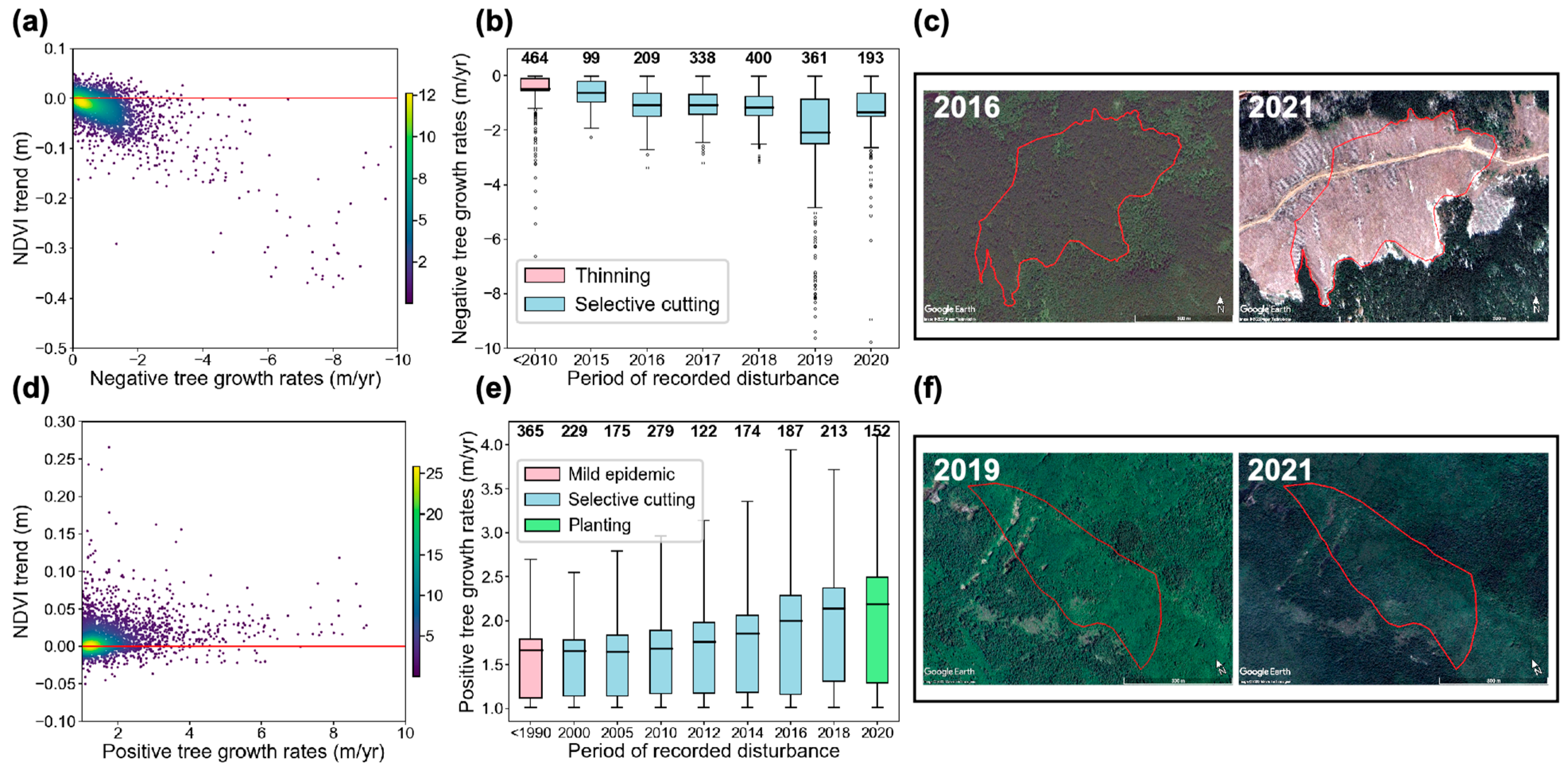
For the analysis of temporal variation in NDVI as a proxy of canopy cover permanence or loss, polygons with negative slopes and positive slopes over 1 m/year were evaluated separately. We found that 13% (2821) of polygons with negative values (tree growth below 0 m/year) underwent tree-canopy loss events, as indicated by a significant negative NDVI slope (p value < 0.05), or by a detected break in the NDVI time series (Figure 6a). Moreover, 6% (1554) of negative polygons have a reported disturbance occurring after the airborne-LiDAR acquisition date, which matches a break in the NDVI time series. Most of the reported disturbances correspond to different types of selective cutting. These results indicate that some negative values in the tree-growth dataset correspond to actual change in canopy height (Figure 6c).
For the forest stands with positive values over 1 m/year, we found that 95% (2961) of polygons correspond with tree-canopy cover gain or permanence as indicated by NDVI slopes that are not significantly different from zero (p value ≥ 0.05), or significant positive NDVI slopes (p value < 0.05), and, in all cases, forest stands that do not register any breaks in the NDVI time series (Figure 6d). Of these polygons, 64% (1896) have at least one reported disturbance event, which mostly occurred before the CHM acquisition date. Most of the reported disturbances correspond to different types of selective cutting and planting processes (Figure 6e). These results indicate that although the estimated extreme-positive tree-growth rates are unlikely to correspond to actual biological rates of gain in tree height, the GEDI data are accurately recording the permanence of tree canopy (Figure 6f). As explained before, a clear source of error in the tree-growth estimations is derived from GEDI data scarcity and the heterogeneity of forest stands. Additionally, a possible source of error that was not explored in this study is related to the horizontal positional uncertainty of the GEDI footprints of approximately ±10 m [61]. This geolocation uncertainty could further bias tree-growth rates, particularly if the GEDI footprints are close to the boundaries of the forest stands, so that the GEDI data are no longer representative of the average tree height of the corresponding forest stand.
4. Discussion
We developed a methodology for detecting tree growth by using GEDI data to extend the temporal coverage of an airborne-LiDAR and forestry dataset. Our results show the capabilities of the GEDI products to accurately characterize forests’ vertical structure and evaluate stand height. Clearly, our study largely benefitted from the detailed forestry inventory information for the study site, considering that such data coverage and availability would be rare in other locations with important forest resources. However, our results show that repeat spaceborne-LiDAR data could facilitate the replication of our methods in other locations, given a sufficient density of footprints.
4.1. Effects of GEDI Data Scarcity
The sparse coverage of the GEDI data constitutes the main limitation of our approach. To overcome data scarcity, we established the forest stand as the unit of analysis and used a pre-established forest stand delineation to aggregate the GEDI footprints. Moreover, a minimum footprint density was determined to guarantee that sufficient data were available to characterize each forest stand polygon. Despite the benefits of an object-oriented approach for upscaling the spatial coverage of the GEDI data, there are clear drawbacks to our methods. First, our analysis was based on the assumption that the forest stands represent a homogeneous group of trees with similar canopy height. While this assumption might work well for some cases, forest stands are likely to have complex vertical structures with heterogenous tree height, resulting in a misrepresentation of average tree-height conditions for these areas due to the sparse GEDI data. Secondly, as our results demonstrate, footprint density alone does not guarantee a good representation of average tree height, since the location of the GEDI footprints inside the forest stand can result in the detection of extreme values of tree height. And, thirdly, the forest stand delineation included in the forestry inventory might not be updated after disturbance events and might not represent current homogeneous patches of forest in the study area. Nevertheless, our study shows that we can infer overall trends in canopy growth or detect disturbance events resulting in changes in overall stand height. Albeit losing the spatial resolution at the scale of the GEDI footprint, we gain accuracy in the estimation of average tree-height conditions by aggregating the data. Additional work to possibly improve our results, would include constructing a forest stand delineation that coincides with the GEDI-data-acquisition time frame by using remote sensing imagery and object detection or image-segmentation processes.
4.2. Tree Growth in the Laurentides Reserve
We estimated an average tree-growth rate for the Laurentides reserve of 0.32 ± 0.23(SD) m/year, which is of the same order of magnitude as estimates from field data corresponding to 0.21 ± 0.12(SD) m/year. The resulting dataset follows expected patterns of tree growth according to year-of-disturbance as proxy for age, and tree species, and although our results include extreme values of tree growth, we were able to determine that some of those extreme values correspond with either recorded disturbance events, in the case of negative rates, or with the permanence of tree cover in a forest stand, in the case of positive trends. These results provide valuable insight into the benefits of using GEDI data for tracking spatio-temporal changes in forest vertical structure and add to the body of knowledge on the capabilities of GEDI data for accurately tracking changes in canopy height [62,63]; however, important caveats and limitations of our results need to be considered.
As mentioned before, the drawbacks of our approach resulted in uncertainty in the estimation of average tree-height conditions for heterogenous forest stands, and the accuracy assessment of the GEDI data indicates overestimation of average tree height for short forest stands, and underestimation for tall forest stands. More importantly, equating increases in canopy height to increases in average tree height is not straightforward, considering the growth patterns of trees, possible seasonal or phenological differences between the GEDI acquisition’s dates, and forest stand-specific characteristics of the canopy structure. In the first place, lateral growth of tree crowns could result in increases in the relative height of the GEDI data, due to changes in the returns of the GEDI signal between years. Similarly, differences in seasonal (for example snow cover) and phenological conditions (for example leaf-off) during the GEDI acquisition date affect the signal returns and could have resulted in erroneous or biased measurements of average tree growth. Unfortunately, due to limitations in data availability, we did not filter the GEDI data by specific months of the year; therefore, further work is required to determine the effects of seasonality on the GEDI data. Finally, the growth signal between forest stands may have affected by the structure of the canopy, where a multi-layered canopy could result in values of relative height and tree growth that do not represent the whole forest stand, but that were caused by growth of the understory vegetation.
These limitations in the GEDI data and our methods may have resulted in uncertainty in the average tree height per forest stand and would have consequently led to error propagation into the tree-growth rates. For these reasons, we consider that our tree-growth estimations should be regarded as general trends of forest dynamics, and that further work is needed to improve the accuracy of tree-growth estimates, for example by considering other relative height metrics, different processing methods, or, as mentioned before, producing new forest stand delineation maps that truly represent homogeneous canopies. Nevertheless, we believe that the GEDI data provides valuable information for detecting changes in canopy height, particularly considering the cost restrictions of producing multitemporal airborne-LiDAR acquisitions for large areas and with high temporal frequency, in contrast to the coverage and repeated pass of the GEDI acquisitions. Moreover, improvements in the accuracy of tree-growth rates from GEDI data could be achieved with longer time series, as this would facilitate the detection of outliers and a robust estimation of trends.
5. Conclusions
This study shows the benefits of integrating airborne- and spaceborne-LiDAR data for monitoring forest tree growth. The use of repeat GEDI acquisitions allowed for us to extend the temporal coverage of the airborne-LiDAR and forestry-field data for the Laurentides wildlife reserve, and to estimate general trends in tree growth. While recognizing the limitations of our methodology, we believe that our approach could be useful for tracking changes in the vertical structure of forests. This study supports the potential of future spaceborne missions, such as the Surface Topography and Vegetation (STV), Target Observable discussed in the U.S. Decadal Survey [38]. Finally, these types of assessments are important when considering the possible future effects of climate change on forest ecosystems services, and the derived feedback on the carbon cycle, as well as the relevance of spatially detailed information on forest tree growth for land and forest resource management.
Author Contributions
Conceptualization, M.S.; methodology, data curation, and investigation, A.P.; original draft preparation A.P.; review and editing, A.P. and M.S.; supervision, M.S. All authors have read and agreed to the published version of the manuscript.
Funding
This work was funded by NASA’s Earth Surface and Interior Focus Area for participation in the Surface Topography and Vegetation Structure Science Team. This work was performed at the Jet Propulsion Laboratory under contract with the National Aeronautics and Space Administration (NASA) (80NM0018D0004).
Data Availability Statement
The GEDI L2A and L2B products are publicly available at the NASA/USGS Land Processes Distributed Active Archive Center (https://lpdaac.usgs.gov/ accessed on 7 March 2023), and the data from the Québec forestry inventory is publicly available at the Québec government data portal (https://www.donneesquebec.ca/ accessed on 12 July 2022). The resulting dataset from this study will be publicly available at Simard’s website (https://landscape.jpl.nasa.gov/).
Acknowledgments
We would like to thank the GEDI mission science team for the data products, and the Government of Québec for the airborne LiDAR and forestry data of the Laurentides Wildlife reserve. All these data are open access, which allowed for the realization of this study.
Conflicts of Interest
The authors declare no conflict of interest.
References
- Neeff, T.; Piazza, M. How countries link forest monitoring into policy-making. For. Policy Econ. 2020, 118, 102248. [Google Scholar] [CrossRef]
- Herold, M.; Johns, T. Linking requirements with capabilities for deforestation monitoring in the context of the UNFCCC-REDD process. Environ. Res. Lett. 2007, 2, 045025. [Google Scholar] [CrossRef]
- Santilli, M.; Moutinho, P.; Schwartzman, S.; Nepstad, D.; Curran, L.; Nobre, C. Tropical deforestation and the Kyoto protocol. Clim. Chang. 2005, 71, 267–276. [Google Scholar] [CrossRef]
- Forneri, C.; Blaser, J.; Jotzo, F.; Robledo, C. Keeping the forest for the climate’s sake: Avoiding deforestation in developing countries under the UNFCCC. Clim. Policy 2006, 6, 275–294. [Google Scholar] [CrossRef]
- Akhtar-Schuster, M.; Stringer, L.C.; Erlewein, A.; Metternicht, G.; Minelli, S.; Safriel, U.; Sommer, S. Unpacking the concept of land degradation neutrality and addressing its operation through the Rio Conventions. J. Environ. Manag. 2017, 195, 4–15. [Google Scholar] [CrossRef]
- Hein, J.; Guarin, A.; Frommé, E.; Pauw, P. Deforestation and the Paris climate agreement: An assessment of REDD+ in the national climate action plans. For. Policy Econ. 2018, 90, 7–11. [Google Scholar] [CrossRef]
- Gren, I.M.; Aklilu, A.Z. Policy design for forest carbon sequestration: A review of the literature. For. Policy Econ. 2016, 70, 128–136. [Google Scholar] [CrossRef]
- Olander, L.P.; Gibbs, H.; Steininger, M.; Swenson, J.; Murray, B.C. Data and Methods to Estimate National Historical Deforestation Baselines in Support of UNFCCC REDD. Options 2007, 4. Available online: https://nicholasinstitute.duke.edu/ecosystem/land/data-and-methods-to-estimate-national-historical-deforestation-baselines-in-support-of-unfccc-redd (accessed on 16 February 2023).
- DeFries, R.; Achard, F.; Brown, S.; Herold, M.; Murdiyarso, D.; Schlamadinger, B.; de Souza, C. Earth observations for estimating greenhouse gas emissions from deforestation in developing countries. Environ. Sci. Policy 2007, 10, 385–394. [Google Scholar] [CrossRef]
- Dolan, K.; Masek, J.G.; Huang, C.; Sun, G. Regional forest growth rates measured by combining ICESat GLAS and Landsat data. J. Geophys. Res. Biogeosci. 2009, 114, 1–7. [Google Scholar] [CrossRef]
- Matula, R.; Knířová, S.; Vítámvás, J.; Šrámek, M.; Kníř, T.; Ulbrichová, I.; Svoboda, M.; Plichta, R. Shifts in intra-annual growth dynamics drive a decline in productivity of temperate trees in Central European forest under warmer climate. Sci. Total Environ. 2023, 905, 166906. [Google Scholar] [CrossRef]
- Lemprière, T.C.; Bernier, P.Y.; Carroll, A.L.; Flannigan, M.D.; Gilsenan, R.P.; McKenney, D.W.; Hogg, E.H.; Pedlar, J.H.; Blain, D. The Importance of Forest Sector Adaptation to Climate Change. 2008. Available online: http://dsp-psd.pwgsc.gc.ca/collection_2009/nrcan/Fo133-1-416E.pdf (accessed on 8 June 2023).
- Chen, H.Y.H.; Luo, Y. Net aboveground biomass declines of four major forest types with forest ageing and climate change in western Canada’s boreal forests. Glob. Chang. Biol. 2015, 21, 3675–3684. [Google Scholar] [CrossRef]
- Finer, M.; Novoa, S.; Weisse, M.J.; Petersen, R.; Mascaro, J.; Souto, T.; Stearns, F.; Martinez, R.G. Combating deforestation: From satellite to intervention. Science 2018, 360, 1303–1305. [Google Scholar] [CrossRef]
- Coops, N.C. Characterizing forest growth and productivity using remotely sensed data. Curr. For. Reports 2015, 1, 195–205. [Google Scholar] [CrossRef]
- Fagan, M.; Defries, R. Measurement and Monitoring of the World’s Forests: A Review and Summary of Remote Sensing Technical Capability, 2009–2015; Resources for the Future: Washington, DC, USA, 2015; Available online: https://www.rff.org/publications/reports/measurement-and-monitoring-of-the-worlds-forests-a-review-and-summary-of-remote-sensing-technical-capability-20092015/ (accessed on 21 February 2023).
- World Resources Institute. Global Forest Watch. 2022. Available online: https://www.globalforestwatch.org/ (accessed on 21 February 2023).
- Hansen, M.C.; Loveland, T.R. A review of large area monitoring of land cover change using Landsat data. Remote Sens. Environ. 2012, 122, 66–74. [Google Scholar] [CrossRef]
- Turubanova, S.; Potapov, P.; Hansen, M.C.; Li, X.; Tyukavina, A.; Pickens, A.H.; Hernandez-Serna, A.; Arranz, A.P.; Guerra-Hernandez, J.; Senf, C.; et al. Tree canopy extent and height change in Europe, 2001–2021, quantified using Landsat data archive. Remote Sens. Environ. 2023, 298, 113797. [Google Scholar] [CrossRef]
- Sinha, S.; Jeganathan, C.; Sharma, L.K.; Nathawat, M.S. A review of radar remote sensing for biomass estimation. Int. J. Environ. Sci. Technol. 2015, 12, 1779–1792. [Google Scholar] [CrossRef]
- Lehmann, E.A.; Caccetta, P.; Lowell, K.; Mitchell, A.; Zhou, Z.-S.; Held, A.; Milne, T.; Tapley, I. SAR and optical remote sensing: Assessment of complementarity and interoperability in the context of a large-scale operational forest monitoring system. Remote Sens. Environ. 2015, 156, 335–348. [Google Scholar] [CrossRef]
- Marshak, C.; Simard, M.; Denbina, M. Monitoring forest loss in ALOS/PALSAR time-series with superpixels. Remote Sens. 2019, 11, 556. [Google Scholar] [CrossRef]
- Solberg, S.; Hansen, E.H.; Gobakken, T.; Næssset, E.; Zahabu, E. Biomass and InSAR height relationship in a dense tropical forest. Remote Sens. Environ. 2017, 192, 166–175. [Google Scholar] [CrossRef]
- Hansen, E.H.; Gobakken, T.; Solberg, S.; Kangas, A.; Ene, L.; Mauya, E.; Næsset, E. Relative efficiency of ALS and InSAR for biomass estimation in a Tanzanian rainforest. Remote Sens. 2015, 7, 9865–9885. [Google Scholar] [CrossRef]
- Simard, M.; Fatoyinbo, L.; Smetanka, C.; Rivera-Monroy, V.H.; Castañeda-Moya, E.; Thomas, N.; Van Der Stocken, T. Mangrove canopy height globally related to precipitation, temperature and cyclone frequency. Nat. Geosci. 2019, 12, 40–45. [Google Scholar] [CrossRef]
- Denbina, M.; Simard, M.; Hawkins, B. Forest Height Estimation Using Multibaseline PolInSAR and Sparse Lidar Data Fusion. IEEE J. Sel. Top. Appl. Earth Obs. Remote Sens. 2018, 11, 3415–3433. [Google Scholar] [CrossRef]
- Santoro, M.; Cartus, O. Research pathways of forest above-ground biomass estimation based on SAR backscatter and interferometric SAR observations. Remote Sens. 2018, 10, 608. [Google Scholar] [CrossRef]
- Lefsky, M.A.; Cohen, W.B.; Harding, D.J.; Parker, G.G.; Acker, S.A.; Gower, S.T. Lidar remote sensing of above-ground biomass in three biomes. Glob. Ecol. Biogeogr. 2002, 11, 393–399. [Google Scholar] [CrossRef]
- Margolis, H.A.; Nelson, R.F.; Montesano, P.M.; Beaudoin, A.; Sun, G.; Andersen, H.-E.; Wulder, M.A. Combining satellite lidar, airborne lidar, and ground plots to estimate the amount and distribution of aboveground biomass in the boreal forest of North America. Can. J. For. Res. 2015, 45, 838–855. [Google Scholar] [CrossRef]
- Boudreau, J.; Nelson, R.F.; Margolis, H.A.; Beaudoin, A.; Guindon, L.; Kimes, D.S. Regional aboveground forest biomass using airborne and spaceborne LiDAR in Québec. Remote Sens. Environ. 2008, 112, 3876–3890. [Google Scholar] [CrossRef]
- Simard, M.; Pinto, N.; Fisher, J.B.; Baccini, A. Mapping forest canopy height globally with spaceborne lidar. J. Geophys. Res. Biogeosci. 2011, 116, 1–12. [Google Scholar] [CrossRef]
- Sothe, C.; Gonsamo, A.; Lourenço, R.B.; Kurz, W.A.; Snider, J. Spatially Continuous Mapping of Forest Canopy Height in Canada by Combining GEDI and ICESat-2 with PALSAR and Sentinel. Remote Sens. 2022, 14, 5158. [Google Scholar] [CrossRef]
- Tokola, T. Remote sensing concepts and their applicability in REDD+ monitoring. Curr. For. Rep. 2015, 1, 252–260. [Google Scholar] [CrossRef]
- Potapov, P.; Li, X.; Hernandez-Serna, A.; Tyukavina, A.; Hansen, M.C.; Kommareddy, A.; Pickens, A.; Turubanova, S.; Tang, H.; Silva, C.E.; et al. Mapping global forest canopy height through integration of GEDI and Landsat data. Remote Sens. Environ. 2021, 253, 112165. [Google Scholar] [CrossRef]
- Fayad, I.; Ienco, D.; Baghdadi, N.; Gaetano, R.; Alvares, C.A.; Stape, J.L.; Scolforo, H.F.; Le Maire, G. A CNN-based approach for the estimation of canopy heights and wood volume from GEDI waveforms. Remote Sens. Environ. 2021, 265, 112652. [Google Scholar] [CrossRef]
- Lang, N.; Kalischek, N.; Armston, J.; Schindler, K.; Dubayah, R.; Wegner, J.D. Global canopy height regression and uncertainty estimation from GEDI LIDAR waveforms with deep ensembles. Remote Sens. Environ. 2022, 268, 112760. [Google Scholar] [CrossRef]
- Dubayah, R.; Goetz, S.J.; Blair, J.B.; Fatoyinbo, T.E.; Hansen, M.; Healey, S.P.; Hofton, M.A.; Hurtt, G.C.; Kellner, J.; Luthcke, S.B. The Global Ecosystem Dynamics Investigation: High-resolution laser ranging of the Earth’s forests and topography. Sci. Remote Sens. 2020, 1, 100002. [Google Scholar] [CrossRef]
- National Academies of Sciences Engineering, and Medicine. Thriving on Our Changing Planet: A Decadal Strategy for Earth Observation from Space; The National Academies Press: Washington, DC, USA, 2018. [Google Scholar]
- Boucher, Y.; Grondin, P.; Noël, J.; Hotte, D.; Blouin, J.; Roy, G. Classification Des Écosystémes Et Répartition Des Forêts Mûres Et Surannées : Le Cas Du Projet Pilote D’aménagement Écosystémique De La Réserve Faunique Des Laurentides; Gouvernement du Québec, Ministère des Ressources naturelles et de la Faune, Direction de la recherche forestière: Quebec, QC, Canada, 2008. [Google Scholar]
- Ministère des Forêts de la Faune et des Parcs. Guide D’utilisation De La Carte Écoforestière Et Des Résultats D’inventaire Écoforestier Du Québec Méridional; Ministère Des Forêts, De La Faune Et Des Parcs, Secteur Des Forêts, Direction Des Inventaires Forestiers: Québec, QC, Canada, 2021.
- Ministère des Forêts de la Faune et des Parcs. Norme De Stratification Écoforestière Quatrième Inventaire Écoforestier Du Québec Méridional; Ministère Des Forêts De La Faune Et Des Parcs: Québec, QC, Canada, 2008. Available online: https://mffp.gouv.qc.ca/nos-publications/norme-stratification-ecoforestiere-quatrieme-inventaire/ (accessed on 9 March 2023).
- Buchhorn, M.; Smets, B.; Bertels, L.; Roo, B.D.; Lesiv, M.; Herold, M.; Fritz, S.; Tsendbazar, N.-E. Copernicus Global Land Service: Land Cover 100m: Collection 3: Epoch 2019: Globe. 2020. Available online: https://zenodo.org/record/3939050 (accessed on 10 March 2023). [CrossRef]
- Ma, Q.; Su, Y.; Guo, Q. Comparison of Canopy Cover Estimations from Airborne LiDAR, Aerial Imagery, and Satellite Imagery. IEEE J. Sel. Top. Appl. Earth Obs. Remote Sens. 2017, 10, 4225–4236. [Google Scholar] [CrossRef]
- Hopkinson, C.; Chasmer, L. Testing LiDAR models of fractional cover across multiple forest ecozones. Remote Sens. Environ. 2009, 113, 275–288. [Google Scholar] [CrossRef]
- Sexton, J.O.; Bax, T.; Siqueira, P.; Swenson, J.J.; Hensley, S. A comparison of lidar, radar, and field measurements of canopy height in pine and hardwood forests of southeastern North America. For. Ecol. Manag. 2009, 257, 1136–1147. [Google Scholar] [CrossRef]
- Helsel, D.R.; Hirsch, R.M.; Ryberg, K.R.; Archfield, S.A.; Gilroy, E.J. Statistical Methods in Water Resources: U.S. Geological Survey Techniques and Methods; U.S. Department of the Interior: Reston, VA, USA; U.S. Geological Survey: Reston, VA, USA, 2020; Chapter A3.
- Theil, H. A Rank-Invariant Method of Linear and Polynomial Regression Analysis. Proc. R. Netherlands Acad. Sci. 1950, 53, 345–381. [Google Scholar] [CrossRef]
- Wilcox, R.R. A Note on the Theil-Sen Regression Estimator When the Regressor Is Random and the Error Term Is Heteroscedastic. Biometrical J. 1998, 40, 261–268. [Google Scholar] [CrossRef]
- Fernandes, R.; Leblanc, S.G. Parametric (modified least squares) and non-parametric (Theil–Sen) linear regressions for predicting biophysical parameters in the presence of measurement errors. Remote Sens. Environ. 2005, 95, 303–316. [Google Scholar] [CrossRef]
- Yu, X.; Hyyppä, J.; Kaartinen, H.; Maltamo, M. Automatic detection of harvested trees and determination of forest growth using airborne laser scanning. Remote Sens. Environ. 2004, 90, 451–462. [Google Scholar] [CrossRef]
- Bowman, D.M.J.S.; Brienen, R.J.W.; Gloor, E.; Phillips, O.L.; Prior, L.D. Detecting trends in tree growth: Not so simple. Trends Plant Sci. 2013, 18, 11–17. [Google Scholar] [CrossRef] [PubMed]
- Sardans, J.; Peñuelas, J. Tree growth changes with climate and forest type are associated with relative allocation of nutrients, especially phosphorus, to leaves and wood. Glob. Ecol. Biogeogr. 2013, 22, 494–507. [Google Scholar] [CrossRef]
- Gorelick, N.; Hancher, M.; Dixon, M.; Ilyushchenko, S.; Thau, D.; Moore, R. Google Earth Engine: Planetary-scale geospatial analysis for everyone. Remote Sens. Environ. 2017, 202, 18–27. [Google Scholar] [CrossRef]
- Holben, B.N. Characteristics of maximum-value composite images from temporal AVHRR data. Int. J. Remote Sens. 1986, 7, 1417–1434. [Google Scholar] [CrossRef]
- Quiros, E.; Polo, M.E.; Fragoso-Campon, L. GEDI Elevation Accuracy Assessment: A Case Study of Southwest Spain. IEEE J. Sel. Top. Appl. Earth Obs. Remote Sens. 2021, 14, 5285–5299. [Google Scholar] [CrossRef]
- Wang, C.; Elmore, A.J.; Numata, I.; Cochrane, M.A.; Shaogang, L.; Huang, J.; Zhao, Y.; Li, Y. Factors affecting relative height and ground elevation estimations of GEDI among forest types across the conterminous USA. GISci. Remote Sens. 2022, 59, 975–999. [Google Scholar] [CrossRef]
- Dorado-Roda, I.; Pascual, A.; Godinho, S.; Silva, C.A.; Botequim, B.; Rodríguez-Gonzálvez, P.; González-Ferreiro, E.; Guerra-Hernández, J. Assessing the accuracy of gedi data for canopy height and aboveground biomass estimates in mediterranean forests. Remote Sens. 2021, 13, 2279. [Google Scholar] [CrossRef]
- Roy, D.P.; Kashongwe, H.B.; Armston, J. The impact of geolocation uncertainty on GEDI tropical forest canopy height estimation and change monitoring. Sci. Remote Sens. 2021, 4, 100024. [Google Scholar] [CrossRef]
- Burns, R.M.; Honkala, B.H. Silvics of North America: 1. Conifers; 2. Hardwoods; U.S. Department of Agriculture, Forest Service: Washington, DC, USA, 1990; Volume 2.
- Pothier, D.; Savard, F. Actualisation Des Tables De Production Pour Les Principales Espèces Forestières Du Québec; Ministère des Ressources Naturelles, Government of Quebec: Quebec, QC, Canada, 1998.
- Dubayah, R.O.; Blair, J.B.; Goetz, S.; Fatoyinbo, L.; Hansen, M.; Healey, S.; Hofton, M.; Hurtt, G.; Kellner, J.; Luthcke, S.; et al. GLOBAL Ecosystem Dynamics Investigation (GEDI) Level 2 User Guide. 2021, 3, 1–25. Available online: https://lpdaac.usgs.gov/documents/986/GEDI02_UserGuide_V2.pdf (accessed on 10 March 2023).
- Milenković, M.; Reiche, J.; Armston, J.; Neuenschwander, A.; De Keersmaecker, W.; Herold, M.; Verbesselt, J. Assessing Amazon rainforest regrowth with GEDI and ICESat-2 data. Sci. Remote Sens. 2022, 5, 100051. [Google Scholar] [CrossRef]
- Guerra-Hernández, J.; Pascual, A. Using GEDI lidar data and airborne laser scanning to assess height growth dynamics in fast-growing species: A showcase in Spain. For. Ecosyst. 2021, 8, 14. [Google Scholar] [CrossRef]
Figure 2.
For the GEDI data with only the quality and degrade flags filtering: (a) location of the 2019 GEDI footprints overlapping the CHM for the year 2019 included in the analysis; (b) correspondence of GEDI RH 99 and CHM percentile 95 with the colors indicating the density of points in the scatterplot, 1:1 line in red for reference; (c) error distribution of the GEDI data in relation to number of detected modes; (d) error distribution of the GEDI data in relation to the GEDI tree cover. For the GEDI data with the complete filtering: (e) correspondence of GEDI RH 99 and CHM percentile 95 with the colors indicating the density of points in the scatterplot, 1:1 line in red for reference; (f) error distribution of the GEDI data in relation to the CHM percentile 95. Number of footprints per-bin are labeled at the top of the boxplots and mean value marked as a black line inside the boxes.
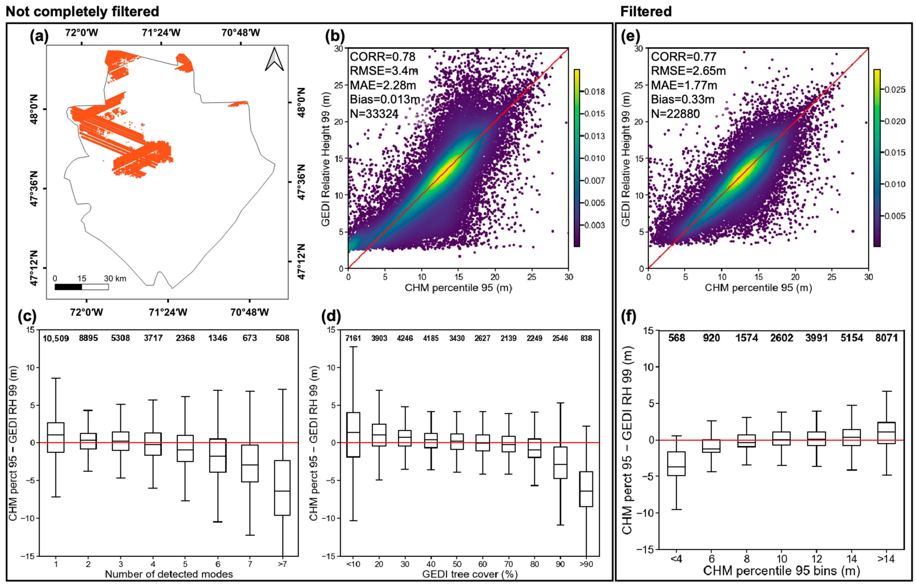
Figure 3.
(a) Location of the forest stands with overlapping CHM and GEDI data for the year 2019 included in the analysis; (b) correspondence of GEDI RH 88 and mean CHM aggregated at the forest stand level with the colors indicating the density of points in the scatterplot, 1:1 line in red for reference. Error distribution according to the following: (c) bins of mean CHM; (d) CHM standard deviation; (e) GEDI point count; (f) GEDI point density. The number of polygons per bin are labeled at the top of the boxplots, the mean value is marked as a black line inside the boxes, and outliers shown as hollow circles.

Figure 4.
Tree-growth estimates for all the forest stands with data in the Laurentides reserve: (a) spatial distribution of the tree-growth estimates; (b) histogram of estimated tree-growth rates compared to the rates from individual trees from permanent sample plots; (c) distribution of the tree-growth rates according to bins of CHM standard deviation, with the mean value marked as a black line inside the boxes and the number of polygons per bin labeled at the top of the boxplots; (d,e) examples of extreme tree-growth rates in forest stands with only one GEDI point and over 3m of CHM standard deviation.
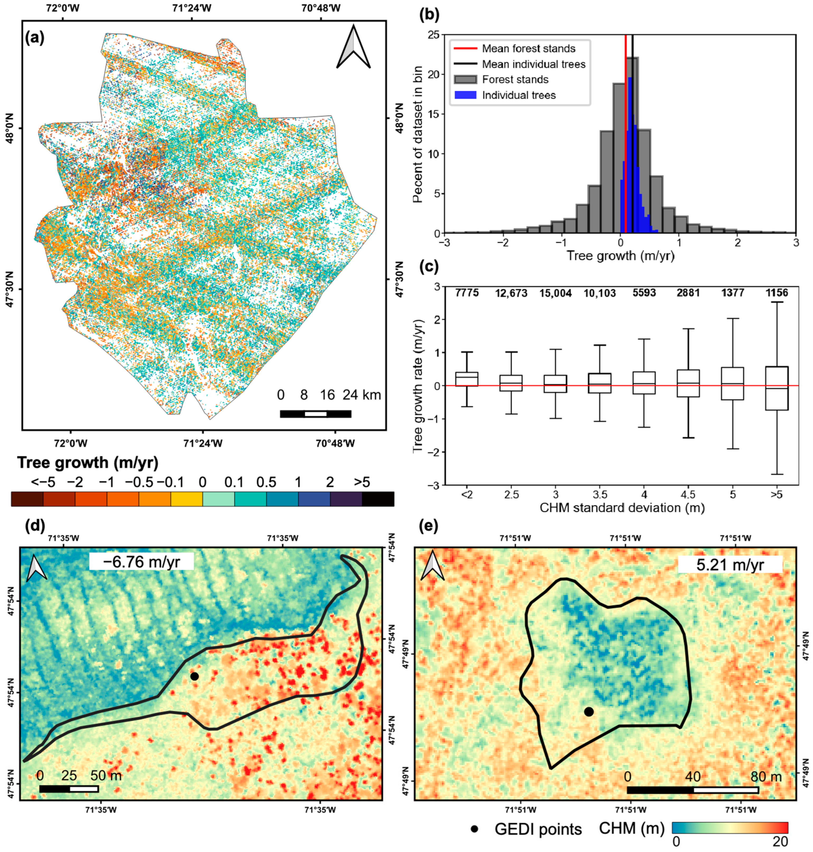
Figure 5.
Tree-growth estimates for forest stands with values between 0 and 1 m/year: (a) spatial distribution of the tree-growth estimates; (b) histogram of estimated tree-growth rates for the forest stands and the individual trees from permanent sample plots; (c) distribution of the tree-growth rates according to the year of disturbance, with the mean value marked as a black line inside the boxes, the number of polygons per bin labeled at the top of the boxplots, and the global mean of the dataset shown as a horizontal red line. Analysis of tree-growth rates for the individual trees from permanent sample plots and forest stands per: (d) species and dominant species, respectively, and (e) forest type. The mean value of each group is labeled and marked inside the boxes with a black line, the number of individual trees or forest stands is labeled at the top of the boxplot, and the global mean of each dataset is shown as a horizontal red line.

Figure 6.
Results for polygons with negative (below 0 m/year) and positive (over 1 m/year) tree-growth rates matching trends in NDVI: (a,d) plots of NDVI trend against the estimated negative and positive tree-growth rate, respectively, with the colors indicating the density of points in the scatterplot; (b,e) distribution of the negative and positive tree-growth rates according to the year of the recorded disturbance, with the most common type of disturbance labeled by color, the mean value marked as a black line inside the boxes, and the number of polygons per bin labeled at the top; (c) before and after of a forest stand with a tree-growth rate of −2.3 m/year calculated between 2015 and 2019, that has a reported disturbance in 2018; (f) before and after of a forest stand with a tree-growth rate of 2.3 m/year calculated between 2019 and 2020 with no visible change in tree canopy cover.

Table 1.
Parameters used for filtering out biased GEDI measurements.
| Parameter | Threshold |
|---|---|
| Degraded flag | ≠0 |
| Quality flag | ≠0 |
| Number of detected modes | =0 OR >7 |
| Elevation of the highest return—TanDEM-X elevation | <−20 m OR >20 m |
| Landsat water persistence | >80 |
| Total canopy cover from GEDI | <5% OR >90% |
| Total Energy | <2000 |
| Last mode energy ÷ energy total | <0.195 |
| For waveforms with only one mode: last mode energy | <2000 |
| For waveforms with only one mode: zcross local energy | <150 |
Table 2.
Tree-growth rates at the forest stand level calculated from LiDAR data and at the individual-tree level calculated from field data.
Table 2.
Tree-growth rates at the forest stand level calculated from LiDAR data and at the individual-tree level calculated from field data.
| Dataset | Tree Growth (m/Year) | Samples | |||
|---|---|---|---|---|---|
| Mean | Min | Max | SD | ||
| All forest stands with data | 0.09 | −9.78 | 11.22 | 0.76 | 56,562 |
| Forest stand with values of 0–1 m/year | 0.32 | 0 | 1 | 0.23 | 31,325 |
| Individual trees from permanent plots | 0.21 | 0 | 0.92 | 0.12 | 3579 |
Disclaimer/Publisher’s Note: The statements, opinions and data contained in all publications are solely those of the individual author(s) and contributor(s) and not of MDPI and/or the editor(s). MDPI and/or the editor(s) disclaim responsibility for any injury to people or property resulting from any ideas, methods, instructions or products referred to in the content. |
© 2023 by the authors. Licensee MDPI, Basel, Switzerland. This article is an open access article distributed under the terms and conditions of the Creative Commons Attribution (CC BY) license (https://creativecommons.org/licenses/by/4.0/).
Share and Cite
MDPI and ACS Style
Parra, A.; Simard, M. Evaluation of Tree-Growth Rate in the Laurentides Wildlife Reserve Using GEDI and Airborne-LiDAR Data. Remote Sens. 2023, 15, 5352. https://doi.org/10.3390/rs15225352
AMA Style
Parra A, Simard M. Evaluation of Tree-Growth Rate in the Laurentides Wildlife Reserve Using GEDI and Airborne-LiDAR Data. Remote Sensing. 2023; 15(22):5352. https://doi.org/10.3390/rs15225352
Chicago/Turabian StyleParra, Adriana, and Marc Simard. 2023. "Evaluation of Tree-Growth Rate in the Laurentides Wildlife Reserve Using GEDI and Airborne-LiDAR Data" Remote Sensing 15, no. 22: 5352. https://doi.org/10.3390/rs15225352
Note that from the first issue of 2016, this journal uses article numbers instead of page numbers. See further details here.