Adversarial Attacks in Underwater Acoustic Target Recognition with Deep Learning Models

Abstract

Deep learning models can produce unstable results by introducing imperceptible perturbations that are difficult for humans to recognize. This can have a significant impact on the accuracy and security of deep learning applications due to their poorly understood interpretability. As a field critical to security research, this problem clearly exists in underwater acoustic target recognition for ocean sensing. To address this issue, this article investigates the reliability of state-of-the-art deep learning models by exploring adversarial attack methods that add small, exquisite perturbations on acoustic Mel-spectrograms to generate adversarial spectrograms. Experimental results based on real-world datasets reveal that these models can be forced to learn unexpected features when subjected to adversarial spectrograms, resulting in significant accuracy drops. Specifically, when employing the iterative attack method, the overall accuracy of all models experiences a significant decrease of approximately 70% for two datasets under stronger perturbations.

1. Introduction

The underwater acoustic target recognition technique is an information processing approach in ocean remote sensing that utilizes sonar-received acoustic signals to extract meaningful characteristics and classify the target type. As human activities in the ocean continue to increase, its application has substantially widened, making it a hot topic in the field of marine research [1,2]. To accurately predict ship types in real marine applications, time–frequency analysis has proven to be beneficial in this task and has made certain achievements [3]. Nevertheless, the challenges stemming from the complex underwater acoustic environment and the intricate sound propagation mechanisms present significant obstacles to underwater acoustic target recognition. These challenges directly impact the performance and accuracy of underwater communication systems and ocean sensing technologies [4,5], further emphasizing the difficulties encountered in this field.

In recent years, the development of artificial intelligence has significantly facilitated the implementation of data-driven methods that are highly effective in accomplishing underwater acoustic target recognition tasks. Deep learning, in particular, has been widely adopted and demonstrated to outperform traditional classifiers [6,7] in recognizing target signals using time–frequency representations extracted from acoustic data. Furthermore, due to its flexible scalability, an increasing number of models with various designs of neural networks are being proposed to further enhance recognition performance. Sun et al. [8] used real-valued and complex-valued ResNet and DenseNet convolutional neural networks (CNN) to recognize underwater target signals, and the satisfactory results have proven the strong ability of CNNs to efficiently extract information embedded in the acoustic signal. Doan et al. [9] also proposed a dense CNN model that is designed to reuse former feature maps for underwater acoustic target recognition, and the obtained results based on real-world datasets have shown its outperformance over other CNN models. To make use of the attention mechanism, Feng et al. [10] proposed a Transformer-based deep learning model for underwater acoustic target recognition, named the UATR-Transformer (UATRT), to fully exploit the information in the Mel-spectrogram, which has achieved comparable performance compared with the CNNs. Moreover, Li et al. [11] utilized transfer learning with the Spectrogram Transformer Model (STM) to recognize a real-world dataset, which further demonstrated the superiority of the Transformer model in extracting discriminative features from input spectrograms. Various learning paradigms have also taken deep learning-based underwater acoustic target recognition to new heights. For instance, in [12], researchers combined self-supervised learning with the Transformer architecture to learn general representations that can be utilized for recognizing underwater acoustic targets. Additionally, Xu et al. [13] also leveraged this learning paradigm to define a mask-modeling pretext task for downstream underwater acoustic target recognition using a variant of Transformer, resulting in significant achievements in this scientific area. These variants of CNNs and Transformers have shown promising results, leveraging convolution and attention mechanisms to extract deep representations for models to make the final prediction, which has shown great potential for real applications with advanced deep learning techniques.

While these models achieve satisfactory recognition accuracy by leveraging spectral information from acoustic spectrograms, the question arises as to whether they are robust enough to withstand various perturbations and maintain consistent performance. This concern naturally leads to security issues when using deep learning models, which can potentially pose significant threats and disasters to various applications and systems [14]. The security concerns may also arise in underwater acoustic target recognition due to interpretability issues, often referred to as adversarial attacks [15,16]. These attacks may have devastating consequences for underwater acoustic target recognition, including the misclassification of critical underwater entities and the degradation of system performance and reliability. As such, it is crucial to evaluate the robustness of the used deep learning models against adversarial attacks, as well as the effectiveness of attack methods. Furthermore, we seek to enhance the interpretability of these models by investigating how they respond to adversarial attacks.

The main contributions of this paper are as follows:

• To the best of our knowledge, this is the first instance of visualizing the extracted features of Transformer-based models for underwater acoustic target recognition, which are believed to perceive spatial structures differently through the use of MHSA rather than convolution operations.
• This is also the first time to introduce adversarial attacks in the area of underwater acoustic target recognition. Based on the real-world underwater acoustic dataset, we generated the adversarial spectrograms by adding a well-designed perturbation on the input time–frequency representation to successfully attack the state-of-the-art (SOTA) deep learning networks for underwater acoustic target recognition, which demonstrates their vulnerability under adversarial attacks. Moreover, we also analyzed how the adversarial attacks influenced the decision-making process of these models through visualization.
• From the perspective of underwater acoustic signal preprocessing, experimental results demonstrate that using the MFCC feature or normalizing time–frequency spectrograms with a standard deviation of 1 can potentially improve the adversarial robustness.

The paper is organized as follows: Section 2 illustrates the related work. Section 3 provides a brief introduction to the framework of CNN and Transformer model-based underwater acoustic target recognition methods. Section 4 presents the adversarial attack methods used to generate adversarial spectrograms to make deep learning models produce inaccurate predictions, as well as a visualization method for interpretability research. The dataset partitions and implementation details are provided in Section 5. The adversarial attack and visualization results on the SOTA models are presented in Section 6. Finally, Section 7 presents the conclusions.

2. Related Work

Adversarial attacks in the realm of deep learning involve deliberately manipulating input data to induce mistakes in a deep learning model. These attacks leverage the susceptibilities of deep learning models, specifically their sensitivity to minute alterations in the input data, which are often imperceptible [17]. In safety-critical areas, weak model robustness can signify vulnerability to adversarial attacks by imperceptible perturbations. Gong et al. [16] successfully disrupted an end-to-end convolutional recurrent network model using adversarial attacks on the original waveform. Kreuk et al. [18] achieved better attack performance against [16] by performing a directed attack on the Mel-scale frequency cepstral coefficient (MFCC) acoustic feature. In [19], the researchers employed various gradient-based adversarial attack algorithms to evaluate the vulnerability of sound event classification models. The experimental findings showcased the effectiveness of these attacks on different models. Furthermore, Joshi et al. [20] used several adversarial methods to attack advanced speech recognition systems, and the attack results demonstrated that these systems are highly vulnerable to adversarial attacks.

This susceptibility problem is mainly attributed to the weak interpretability of deep learning models [21]. The features extracted by deep learning models automatically may not be comprehensible to human recognition systems, and the underlying principles to obtain these features are difficult to investigate. To address this issue, researchers have focused on improving the interpretability of deep learning models and their applications. For example, Lauritsen et al. [22] introduced an early warning score system that can detect acute critical illness while explaining its complex decision-making process. Jiménez-Luna et al. [23] proposed explainable AI algorithms for improving the interpretability of deep learning models in molecular sciences. In the underwater acoustic field, an efficient and interpretable feature set was identified and evaluated using a BP neural network [24], the experimental results demonstrated the validity of these features for underwater acoustic target recognition. To make use of the attention mechanism, Xiao et al. [25] suggested using an attention-based neural network to enhance interpretability during target detection and recognition. However, the interpretability of Transformer models with the multi-head self-attention (MHSA) mechanism for recognizing underwater acoustic targets has not yet been explored.

3. Preliminaries

In this section, we present the general framework of the underwater acoustic target recognition methods based on CNN and Transformer models to show their respective mechanisms for recognizing underwater acoustic signals.

3.1. CNN Models

CNN models have been extensively utilized in underwater acoustic target recognition due to their powerful feature extraction ability through kernel sliding on the acoustic spectrogram. Figure 1 shows the framework of an example CNN-based approach that consists of data preprocessing, a CNN architecture for feature extraction, and target classification. Data preprocessing involves obtaining time–frequency representations in the form of acoustic spectrograms, which can be achieved by short-time Fourier transform (STFT). Then the convolution block in CNN receives a spectrogram of size (c, t, f) as the model input, where c represents the channel and f is the number of frequency bins.

An example convolution block consists of a convolution layer and a pooling layer. Specifically, the convolution layer convolutes the data $X_l$ from the previous layer with a combination of convolution kernels, represented by kernel core $K_l$ of size $[C_l,C_{l+1},K_t,K_f]$ in layer l, to generate the data $X_{l+1}$ of the next layer. During this process, each neuron acts as a filter with shared weights across the acoustic spectrogram, which allows the convolutional block to focus more on local structures. The convolution process for converting $X_l$ to $X_{l+1}$ can be expressed as [26]:

$$\begin{array}{cc}\hfill X_{l+1}[c,t,f]=& \sum _{c_i=0}^{C_l-1}\sum _{k_t=0}^{K_t-1}\sum _{k_f=0}^{K_f-1}{K}_l\left[c_l,c,k_t,k_f\right]\times X_l\left[c_l,t+k_t,f+k_f\right].\hfill \end{array}$$

(1)

In which, $0⩽k_t⩽K_{t-1},0⩽k_f⩽K_{f-1}$. Meanwhile, the pooling layer carries out subsampling, utilizing either average pooling or max-pooling methods. Using average pooling as an example, a window of data $X_l$ in layer l is averaged to obtain $X_{l+1}$ as follows:

$$\begin{array}{c}\hfill X_{l+1}[c,t,f]={\displaystyle \frac{1}{K_t{K}_f}}\sum _{k_t=0}^{K_t-1}\sum _{k_f=0}^{K_f-1}{X}_l[c,K_{t}t+k_t,K_{f}f+k_f].\end{array}$$

(2)

After multiple combinations of convolutional and pooling layers, the feature map of the final layer is considered to have captured the deepest patterns in the acoustic spectrogram.

In order to categorize different ship types, a fully connected layer is commonly used as the classifier, with the predicted ship type being determined based on the highest probability. Overall, CNNs concentrate on the local features of spectrograms using convolutional kernels, resulting in a local information model for recognizing underwater acoustic signals.

3.2. Transformer Models

In contrast to CNNs, the Transformer architecture employs the MHSA mechanism instead of convolution. This allows for global content-dependent interactions within time–frequency representations and better model relationships across long ranges. Figure 2 illustrates the framework of an example Transformer-based underwater acoustic target recognition.

Although the model input remains a $t\times f$ spectrogram, tokens are utilized as fundamental elements for self-attention computation. Practically, informative tokens can be generated through various tokenization methods, with regular tokenization being the most widely used in Vision Transformer [27]. The approach involves convolutional operations that divide the acoustic spectrogram into square patches, which are then flattened into embedded sequences. To preserve the spatial positional information, each token is attached with a well-designed positional embedding that can be formulated as [28]:

$$\begin{array}{cc}\hfill & P{E}_{(pos,2i)}=sin\left(pos/10,{000}^{2i/D_{Embedding}}\right)\hfill \\ \hfill & P{E}_{(pos,2i+1)}=cos\left(pos/10,{000}^{2i/D_{Embedding}}\right),\hfill \end{array}$$

(3)

where $pos$ is the order of the token sequences, $i\in [1,D_{Embedding}/2]$, $D_{Embedding}$ is the token embedding to encode the patch. The scaling factor value of 10000 is used to determine the strength of positional differences, which is recommended by [28] and has been shown to be effective in many tasks. In this case, the original acoustic spectrogram is encoded as tokens with positional information and then processed by L Transformer encoders.

Importantly, the MHSA block computes inter-token relations in Transformer encoders and is essential for learning diverse information from input sequences. In the first encoder $l_0$, tokenized input features are transformed into $X_0$ with the size of $P\times D_{Embedding}$ tokens; $P=t/K_t\times f/K_f$ is the number of tokens, where $K_t$ and $K_f$ are the kernel sizes used to split the spectrogram. Subsequent encoders project $X_{l-1}$ onto the query set $Q_h$, the key set $K_h$, and the value set $V_h$ to compute attention distribution via the dot product, which can be expressed as follows:

$$\begin{array}{c}{Q}_h,K_h,V_h=X_{l-1}{W}_h^Q,X_{l-1}{W}_h^K,X_{l-1}{W}_h^V\\ Attn\left(Q_h,K_h,V_h\right)=softmax\left(\frac{Q_h{K}_h^T}{\sqrt{D_{attn}}}\right)V_h.\end{array}$$

(4)

where $W_h^Q$, $W_h^K$, and $W_h^V$ denote the learnable projection matrices, H is the number of heads, $h\in [1,H]$ represents which head to be calculated, and the dimension of attention embedding is defined as $D_{attn}=D_{Embedding}/H$. Since MHSA can capture long-range dependencies between different positions in the token sequence, after applying MHSA and multi-layer perceptron (MLP) in L Transformer encoders, a global feature map of size $P\times D_{Embedding}$ that contains discriminative time–frequency information is obtained.

In a standard Transformer, the [CLS] token is utilized to consolidate classification information from other tokens, and is subsequently fed into an MLP head for final prediction. To improve recognition performance by grouping all tokens together in the frequency domain, ref. [10] proposed a token-pooling classifier to predict ship types, which is believed to produce superior results for recognizing acoustic signals. Although underwater acoustic target recognition using Transformer models is still nascent, the remarkable recognition results achieved are anticipated to improve even further with the emergence of diverse variant structures.

4. Methodology

In the area of underwater acoustic target recognition, time–frequency spectrograms are commonly used to intuitively represent acoustic signals, making it essentially a pattern recognition problem. By the time–frequency analysis, the signal waveform is transformed into a spectrogram $\mathit{x}$. Assuming the corresponding label of the original spectrogram $\mathit{x}$ is y, this problem can be approached from a deep learning perspective by iterative training to obtain optimal parameters $\theta$. The optimization objective can be expressed as follows:

$$\begin{array}{c}\hfill \underset{\theta }{\mathrm{argmin}}\mathcal{L}(f(\theta ,\mathit{x}),y),\end{array}$$

(5)

where f represents the deep learning model used for recognition, $\mathcal{L}$ is the loss function to well estimate the differences between label y and the model output $f(\theta ,\mathit{x})$. By training multiple epochs with an optimizer, the loss $\mathcal{L}$ is minimized and the optimal parameters $\theta$ can be determined.

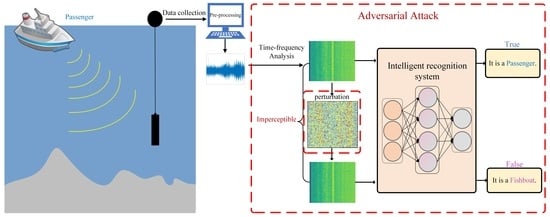
As shown in Figure 3, the original spectrogram is transformed into an adversarial spectrogram by adding a perturbation with the same shape after an adversarial attack. When the adversarial spectrogram is fed into the target deep learning model, the misclassification occurs because the model is deceived by the adversarial spectrogram, which has the ability to make the model predict an incorrect label $y^{\prime }$ with high confidence. In this context, the loss function in Equation (5) is redefined as a maximization problem to find the adversarial spectrogram $\widehat{\mathit{x}}$ for the given input $\mathit{x}$, which can be formulated as follows:

$$\begin{array}{r}\underset{\widehat{\mathit{x}}}{\mathrm{argmax}}\mathcal{L}\left(f\left(\theta ,\widehat{\mathit{x}}\right),y\right)\\ \widehat{\mathit{x}}=\mathit{x}+ϵ,\end{array}$$

(6)

where the added perturbation $ϵ$ is intentionally small to be imperceptible by the human recognition system. Therefore, the resulting adversarial spectrogram $\widehat{\mathit{x}}$ is exploited as a blind spot in the training algorithm, which makes the deep learning model fail to obtain the optimal $\theta$. This happens because the direction of gradient descent is misled, resulting in a significant drop in recognition accuracy, and ultimately achieving the goal of attack.

4.1. Adversarial Attack

The process of generating adversarial spectrograms described above is known as an adversarial attack. In practice, adversarial attacks can be classified into targeted and untargeted attacks based on their goal orientation during the construction of the adversarial spectrogram. In the field of underwater acoustic target recognition, the existing focus is only on inducing mistakes to fool the intelligent system without specific targeting. Therefore, this paper considers only untargeted attacks to explore the influence of natural adversarial attacks. The main objective is to ensure that the adversarial spectrograms generated can produce incorrect predictions when compared to the original samples.

To investigate the effectiveness of attacks in underwater acoustic target recognition, we employ two methods: the basic one-step attack, Fast Gradient Sign Method (FGSM) [29], and the Iterative Projected Gradient Descent (PGD) [15]. Both methods are used to generate adversarial spectrograms, with their modifications constrained by the ${\parallel \parallel }_{\infty }$ norm. The PGD iterative attack approach updates the adversarial spectrogram multiple times, avoiding local optima compared to FGSM. However, it is more time-consuming as it requires constant acquisition and updating $\theta$ of the target model.

4.1.1. Fast Gradient Sign Method

As the fundamental adversarial attack method, FGSM is a gradient-based adversarial attack algorithm that can be used to generate adversarial spectrograms for attacking target recognition models in the underwater acoustic. Unlike backpropagation gradients that minimize loss $\mathcal{L}$, FGSM exploits the rising gradient of the input spectrogram to adjust the model weights $\theta$ and maximize the loss, as shown in Equation (6), thereby performing the attack. In a white-box environment with knowledge of the target model and dataset distribution, FGSM finds the gradient direction and multiplies it by the $\alpha$ step size to obtain the perturbation $ϵ$. Adding this perturbation to the original input produces the adversarial spectrogram generated by FGSM, capable of leading to misclassification of the model with high probability.

Assuming the spectrogram transformed by the acoustic signal is denoted as $\mathit{x}$, the true target label is denoted as y, and a deep learning model f is used for classification, where $f\left(x\right)$ represents the predicted output of $\mathit{x}$ under the target model, the process of generating the adversarial spectrogram with FGSM can be formulated as

$$\begin{array}{c}ϵ=\alpha ·\mathrm{sign}\left({\nabla }_x\mathcal{L}(f\left(\mathit{x}\right),y;\theta )\right)\\ \widehat{\mathit{x}}=\mathit{x}+ϵ.\end{array}$$

(7)

The adversarial spectrogram $\widehat{\mathit{x}}$ is the original example $\mathit{x}$ with a small perturbation of size $ϵ$ added in the direction of the gradient of the loss function $\mathcal{L}\left(f\right(\mathit{x}),y;\theta ))$, where sign$(·)$ provides the direction for perturbing the input that maximizes loss, ultimately leading to misclassification.

4.1.2. Project Gradient Descent

Compared to the FGSM attack, the PGD algorithm utilizes a multi-step approach with random initialization to generate adversarial spectrograms. PGD performs iterative backward and forward propagations, starting from a random initialization point and using the FGSM at each step. At each iteration, PGD calculates the perturbation based on the gradient and accumulates it onto the embedding layer. If the perturbation exceeds a given range, it is projected back onto the permitted range. Finally, the original gradient is updated by accumulating the gradient computed in the last step.

Specifically, PGD iteratively updates the adversarial spectrogram ${\widehat{\mathit{x}}}_t$ from the original acoustic spectrogram $\mathit{x}$; each update involves projecting the previous data ${\widehat{\mathit{x}}}_{t-1}$ plus a small step, sized $\alpha$ times the sign of the gradient ${\nabla }_{{\widehat{\mathit{x}}}_t}\mathcal{L}(f\left({\widehat{\mathit{x}}}_t\right),y;\theta )$ onto the ${\parallel L\parallel }_{\infty }$ ball centered at $\mathit{x}$ with the $\delta$ radius. The projection is performed using an indicator function ${\mathbf{1}}_{\{\parallel \mathit{r}+{\widehat{\mathit{x}}}_t-\mathit{x}{\parallel }_{\infty }\le \delta \}}$, $\mathit{r}$ is the perturbation vector, and the final adversarial spectrogram ${\widehat{x}}_t$ is obtained after T iterations. In this algorithm, ${\widehat{\mathit{x}}}_0=\mathit{x}$ is the initial state of the input, $\delta$ is the maximum perturbation budget, T is the number of iterations, $\alpha$ is the step size, and ${\Pi }_{[\mathit{x}-\delta ,\mathit{x}+\delta ]}(·)$ is a projection operator that maps an input to the ${\parallel L\parallel }_{\infty }$ constraint set $[\mathit{x}-\delta ,\mathit{x}+\delta ]$. The process of PGD (in regard to iteratively finding the adversarial spectrogram) can be expressed as follows:

$$\begin{array}{cc}\hfill {\widetilde{\widehat{\mathit{x}}}}_0& =\mathit{x}\hfill \\ \hfill {\widehat{\mathit{x}}}_{t+1}& ={\Pi }_{[\mathit{x}-\delta ,\mathit{x}+\delta ]}({\widehat{\mathit{x}}}_t+\alpha ·\mathrm{sign}\left({\nabla }_{{\widehat{\mathit{x}}}_t}\mathcal{L}(f\left({\widehat{\mathit{x}}}_t\right),y;\theta )\right)·{\mathbf{1}}_{\{\parallel \mathit{r}+{\widehat{\mathit{x}}}_t-\mathit{x}{\parallel }_{\infty }\le \delta \}})\hfill \\ \hfill {\widehat{\mathit{x}}}_T& ={\widehat{\mathit{x}}}_{T-1}.\hfill \end{array}$$

(8)

In summary, the FGSM is a straightforward yet effective approach used for quickly generating the adversarial spectrogram. By adding perturbations to input time–frequency representation based on the rising gradients, FGSM can generate adversarial spectrograms that are often successful in fooling deep learning models to misclassify the ship types. On the other hand, the PGD algorithm is considered a more powerful and robust method for crafting an adversarial spectrogram since it is an iterative approach used by taking multiple small steps in the direction of the gradient until convergence is reached. It is worth noting that the clamp operation typically used in a standard FGSM and PGD is not necessary for acoustic spectrograms since they involve spectral power rather than actual pixel values.

4.2. GradCAM Visualization

As the underwater acoustic target recognition is essentially a pattern recognition task, the gradient-weighted class activation mapping (GradCAM) algorithm [30] can be naturally employed for an input spectrogram to highlight the regions of interest.

To recognize underwater acoustic signals, a time–frequency spectrogram is first passed through a deep learning model to produce feature maps. The gradients of the output class score to determine the ship type are then computed in the target layer. By averaging the gradients over the spatial dimensions, the importance of each feature map is determined, and finally, these computed importance scores are summed to generate a heatmap that highlights the most concerned areas in the input spectrogram for the decision of the target model.

Specifically, let $f_k(x,y)$ be the activation map of the target layer of CNNs or Transformers for channel k, and ${\alpha }_c^k(x,y)$ be the weighted global average pooling of $f_k(x,y)$, which captures the importance of the feature map for ship class c. The weight for each feature map location $(x,y)$ is obtained by back-propagating the gradient of the output probability with respect to $f_k(x,y)$:

$$\begin{array}{c}\hfill {\alpha }_c^k(x,y)={\displaystyle \frac{1}{Z}}{\displaystyle \frac{\partial y^c}{\partial f_k(x,y)}},\end{array}$$

(9)

where $y^c$ is the output probability and Z is a normalization constant. Then, the GradCAM heatmap for c is computed as a weighted combination of the activation maps:

$$L_{GradCAM}^c=\mathrm{ReLU}(\sum _{x,y}{\alpha }_c^k(x,y)f_k(x,y)),$$

(10)

where ReLU is the rectified linear unit function.

For underwater acoustic target recognition, spectrograms contain valuable time–frequency information that can reveal distinct features among different types of ships. However, these features may not be easily noticeable. In such cases, GradCAM can help visualize the relevant parts of a spectrogram that deep learning models rely on to make recognition decisions.

5. Experimental Setups and Implementation Details

In this section, we present the experimental setups of the datasets and implementation details.

5.1. Datasets

Two real-world datasets, the ShipsEar [31] and the DeepShip [32] with different sampling rates (52,734 Hz and 32,000 Hz), are used in this study. Before model input, both waveforms are downsampled to 16,000 Hz. To balance the feature size, computational resources, and recognition accuracy, all of the full audio recordings in both datasets were segmented into 5-s intervals. Moreover, 70% of these segments were used for training, while the remaining 30% were used for testing, following a widely-used split approach [9,10]. The details of the two datasets can be seen in

Table 1. Dataset partition of the ShipsEar dataset. The categorization follows the operation in [31]; all vessel types were merged into four experimental classes (based on vessel size) and one background noise class.

Class	Ship Types	Training Sample	Testing Sample
A	Fish boats, trawlers, mussel boats, tugboats, dredger	182	83
B	Motorboat, pilot boat, sailboat	196	79
C	Passengers	210	90
D	Ocean liner, RORO	215	85
E	Background noise	204	96

and

Table 2. Dataset partition of the DeepShip dataset. The categorization follows the operation in [32]; all vessel types were merged into four experimental classes.

Class	Ship Types	Training Sample	Testing Sample
A	Cargo	1766	734
B	Passengers	1773	727
C	Tanker	1710	790
D	Tug	1751	749

.

Feature extraction is a crucial factor in achieving high recognition accuracy in underwater acoustic target recognition. Particularly, the use of Mel-spectrogram based on Mel-Fbanks in previous studies [8,10,11] has shown its effectiveness in enhancing low-frequency signal resolution through nonlinear mapping [8]. Therefore, we chose to adopt the Mel-Fbank spectrogram as the input for our experiments to remain consistent with the literature. To extract Mel-spectrogram features, the magnitude of its complex-valued Fourier transform is first calculated by applying STFT to windowed segments. Triangular filters are then applied to the STFT coefficients to approximate the Mel-scale of human perception. The resulting Mel-spectrogram is computed by multiplying the filterbank energies $F(i,k)$ with the STFT coefficients $X(k,m)$ across all frequency bins and time frames. The filterbanks are defined with triangular functions, which are formulated as follows:

$$F(i,k)=\left\{\begin{array}{cc}0\hfill & \mathrm{if}k<f[i-1]\hfill \\ \frac{k-f[i-1]}{f\left[i\right]-f[i-1]}\hfill & \mathrm{if}f[i-1]\le k<f\left[i\right]\hfill \\ \frac{f[i+1]-k}{f[i+1]-f\left[i\right]}\hfill & \mathrm{if}f\left[i\right]\le k<f[i+1]\hfill \\ 0\hfill & \mathrm{if}f[i+1]\le k\hfill \end{array}\right.$$

(11)

where $f\left[i\right]$ is the center frequency of the i-th Mel bin. The entire procedure can be expressed mathematically as:

$$M(k,m)=\sum _{i=0}^{N-1}F(i,k)\times X(i,m),$$

(12)

where N is the number of Mel frequencies. To further extract MFCC features [33], the discrete cosine transform (DCT) is applied to the Mel-Fbanks logarithm to obtain cepstral coefficients, which can effectively concentrate energy and compress data.

$$C(n,m)=\sum _{k=0}^{N-1}{log}_{10}\left(M(k,m)\right)cos[\pi n(k-0.5)/N].$$

(13)

The cepstral coefficients are then adjusted through liftering and output as an MFCC feature vector.

$$\begin{array}{cc}\hfill L\left(n\right)=& 1+\frac{\gamma }{2}sin(\frac{n\pi }{\gamma })\hfill \\ \hfill \mathrm{MFCC}\left(n\right)& =\sum _{m=1}^{M}C\left(m\right)·L\left(n\right),\hfill \end{array}$$

(14)

where $\gamma$ is a constant chosen empirically.

5.2. Implementation

In our study, all experiments were conducted on a computer with an Nvidia GeForce RTX 3090 GPU and a Core i9-10900K CPU using PyTorch 1.8.0 and Python version 3.8. Our experiments evaluate four representative deep learning models for the recognition of underwater acoustic targets and adversarial attacks.

• ResNet18 [34]: ResNet18 has demonstrated excellent performance in recognizing different underwater signals by extracting high-level features using residual connections [8].
• DenseNet169 [35]: DenseNet169 has also shown promising results in underwater acoustic target recognition tasks [8], as its dense connections enable effective feature reuse and propagation.
• STM [11]: Inspired by [36], the STM uses the standard Transformer architecture to extract meaningful features from acoustic spectrograms.
• UATRT [10]: UATRT is a modified Transformer based on hierarchical tokenization to extract discriminative features for underwater acoustic target recognition.

The model with the best recognition accuracy from five time experiments is chosen as the target model to recognize the adversarial spectrograms generated from testing data. To speed up training convergence, the input Mel-spectrogram is normalized according to corresponding references. For Transformers, the dataset mean is 0, and the standard deviation (Std) is 0.5, while for CNNs, the mean is also 0, but the Std is set to 1. Note that all models in our study receive 1D Mel-fbank features of sizes B, 1, 512, 128 as input. These features are extracted from 5s signal segments. The models then output a probability vector, where the highest probability corresponds to the predicted ship type. Moreover, we use the cross-entropy (CE) loss as the loss function, which can be expressed as follows:

$$\begin{array}{c}\hfill \mathcal{L}=-y+log\left(\sum _{j}exp\left(x\left[j\right]\right)\right).\end{array}$$

(15)

where y is the ground-truth of sample x, and $x\left[j\right]$ is the probability of class j output, respectively, $j\in [1,C]$, and C is the number of ship classes.

As a commonly used metric, the overall accuracy is chosen to evaluate the recognition performance, which is computed by dividing the sum of true positives (TPs) aand true negatives (TNs) by the total number of samples, including true positives, true negatives, false positives (FPs), and false negatives (FNs):

$$\mathrm{overall}\mathrm{accuracy}=\frac{TP+TN}{TP+TN+FP+FN}.$$

(16)

6. Experimental Results and Discussion

In this section, we first show the attack performance under various perturbations using the aforementioned deep learning models. Then, we demonstrate the attack performance with different time–frequency spectrograms and different normalization methods using these models. Additionally, we use the GradCAM algorithm for heatmap visualization to illustrate how the adversarial attack affects the model predictions. Finally, the effective attacks are evaluated to demonstrate their invisibility.

6.1. Attack Performance under Different Perturbations

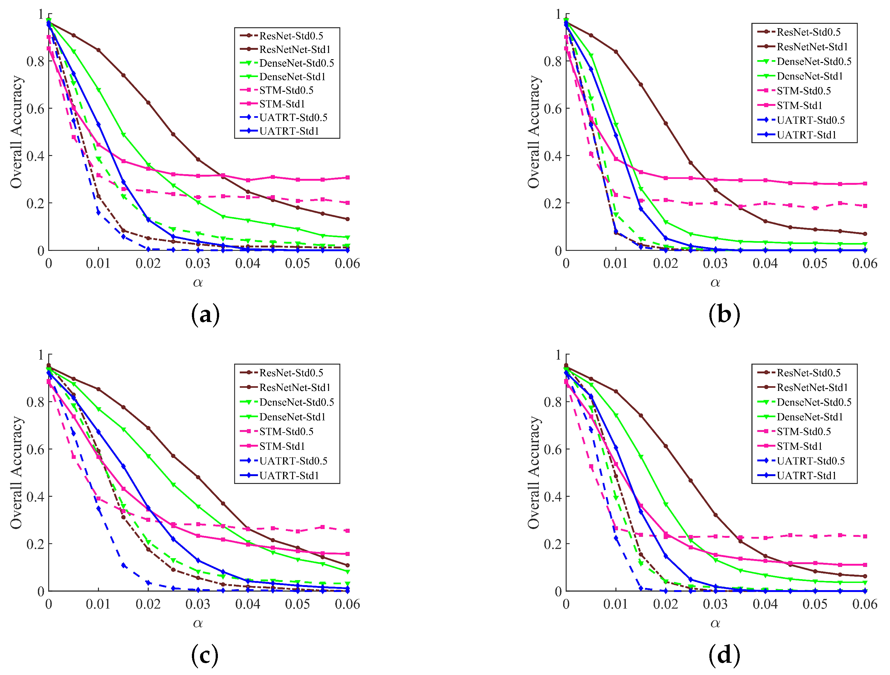
In the initial experiment, to measure the attack performance under varying perturbations corresponding to different step sizes, $\alpha$, the impact of both FGSM and PGD on the overall recognition accuracy is depicted in Figure 4. The larger step size, $\alpha$, indicates that a stronger perturbation is added to the original spectrogram. From Figure 4a,b, we can see clearly that all models have achieved over 90% accuracy with ShipsEar when there is no attack ($\alpha =0$), and 78% with DeepShip, as shown in Figure 4c,d. As $\alpha$ increases, the overall accuracy of all models significantly drops below 25% for ShipsEar and 20% for DeepShip under stronger perturbations ($\alpha =0.06$), which indicates the deep learning-based recognition models are vulnerable to adversarial spectrograms; thus, the adversarial attacks of FGSM and PGD are effective to influence target recognition.

For the four deep learning models, the attack has a more significant impact on Transformer models when $\alpha <0.03$. Among Transformers, the UATRT is more vulnerable to attack than the STM, whose recognition accuracy gradually tends to be stable as $\alpha$ increases over 0.03. It is possible that the UATRT lacks some generalization, although it can achieve the best recognition results under no attack; therefore, it is sensitive to unseen adversarial samples. For the STM, which obtains the lowest accuracy using both datasets without attacks, the accuracy of the model decreases significantly when $\alpha$ is 0.005, and as the perturbation further increases, the overall accuracy reaches around 20% for ShipsEar and 15% for DeepShip. For CNNs, the accuracy obtained by DenseNet decreases significantly faster than that of ResNet, which indicates that DenseNet is more vulnerable to adversarial attacks than ResNet. In particular, Figure 4a shows that the recognition accuracy of CNNs under the FGSM attack is likely to decrease further, but larger values of $\alpha$ may be detectable to humans. Moreover, it is shown that the iterative method, PGD, has a much stronger attack ability compared to the one-step method, FGSM. Using PGD attacks, the recognition accuracy of ResNet, DenseNet, and UATRT can be significantly reduced to nearly 0% using the DeepShip dataset.

To further analyze the attack performance on different ship types, Figure 5 and Figure 6 show the confusion matrices of the four models before and after the attack with an $\alpha =0.06$ value. We mention that the displayed confusion matrix is consistent with the corresponding accuracy shown in Figure 4. Generally, compared with the FGSM attacks shown in column 2, PGD—shown in column 3—can lead to a significant increase in the number of misclassified ships, which further indicates its stronger attack performance. For ShipsEar, when there is no adversarial attack, it can be seen from column 1 that all models can correctly recognize most ship types. However, as shown in columns 2 and 3 (where adversarial attacks are present), it is evident that all models struggle to distinguish between Class B and Class C, demonstrating that the distance between Class B and Class C targets in the feature space is closer, making it more probable to result in misclassification between the two classes. For the DeepShip dataset shown in Figure 6, without adversarial attacks, ResNet, DenseNet, and UATRT can accurately identify most ship types, but Tanker ships are more prone to misclassification. Meanwhile, STM has a relatively higher probability of misclassifying tanker ships and cargo. Moreover, we can observe that a significant number of tanker ships are misclassified as cargo during both FGSM and PGD adversarial attacks for all models, indicating a close feature similarity between tanker and cargo ships.

6.2. Attack Performance under Different Features

The influence of time–frequency representations on attack performance is a subject of interest, as it is known to vary across different feature spaces. In this study, we conducted a comparison of attack performances using the MFCC feature. To simplify our experiment, we selected the ShipsEar dataset.

From Figure 7, it is evident that employing diverse features can result in varied adversarial impacts on the target model. Specifically, the MFCC feature exhibits greater robustness against attacks than Mel-Fbank, particularly when $\alpha <0.04$. When no attack is present, the MFCC yields an accuracy of approximately 92% for ResNet, DenseNet, and UATRT models, while STM achieves nearly 90% accuracy, which is slightly lower than Mel-Fbank. As $\alpha$ increases, the recognition accuracy of CNNs with the MFCC feature drops below 20% when $\alpha =0.06$. Moreover, Transformers with the MFCC exhibit significantly reduced accuracy (below 30%). Among Transformers, UATRT is more vulnerable than STM when both features are used with an accuracy gap of over 20% ($\alpha =0.06$).

Furthermore, our results indicate that the PGD attack method outperforms FGSM, as shown by the more rapid accuracy drop in Figure 7b. It is worth noting that while increasing perturbation levels may further decrease the recognition accuracy of CNNs, it may also make the attack less stealthy, highlighting the trade-off between accuracy and stealthiness in adversarial attacks.

Overall, the experimental results demonstrate that feature choice plays a crucial role in determining the success rate of adversarial attacks. Generally, we find that the MFCC feature is more robust against adversarial attacks than Mel-Fbank. We attribute this difference to the use of DCT in the MFCC feature extraction process; DCT can compress frequency information into a lower-dimensional space, which can effectively reduce the impact of partial perturbation and enhance the robustness against adversarial perturbations.

6.3. Attack Performance under Different Normalization Methods

As adversarial attack methods rely on input gradients, further investigations into the impact of normalization methods on input Mel-spectrograms are conducted. To simplify our study, we focused on the ShipsEar dataset and conducted experiments on spectrogram normalization with Std values of 1 and 0.5.

Based on the results shown in Figure 8, it is evident that using a Std of 1 achieves better recognition accuracy than using a value of 0.5 under adversarial attacks. This could be due to the fact that reducing the Std to 0.5 can amplify high-frequency perturbations, making them more prominent in the time–frequency representations. This observation could be attributed to the fact that reducing the normalization Std to 0.5 can amplify high-frequency perturbations, making them more prominent in the time–frequency representations. Specifically, a lower normalization Std reduces the spread of the data points around the mean, resulting in a higher concentration of values around the mean. Consequently, this higher concentration of values can amplify the impact of high-frequency perturbations, leading to reduced model robustness against adversarial attacks.

Regarding the deep learning models, ResNet’s ability to resist adversarial attacks significantly decreases compared to other models when using a spectrogram normalization Std of 0.5, resulting in a sharp drop in recognition accuracy with both features. When $\alpha$ is 0.06, STM models show higher adversarial robustness than other models. This observation suggests that a pure Transformer model is more resilient to larger adversarial attacks due to its ability to learn higher-level representations. Specifically, when using MFCC features, normalizing spectrogram data with an Std of 1 achieves better accuracy with the STM model when $\alpha <0.025$. However, when $\alpha >0.025$, using STM with a spectrogram normalization Std of 0.5 demonstrates better robustness to adversarial perturbations.

Moreover, UATRT-Std0.5 is highly vulnerable to adversarial perturbations when using both Mel-Fbank and MFCC features, which indicates that the modifications made to the standard Transformer model may have compromised its robustness against adversarial attacks. This finding aligns with similar observations in other scientific domains [37]. In contrast, the DenseNet-Std1 model exhibited greater robustness than other models when using different features with varying normalization Std values. This may be attributed to its dense architecture, which incorporates multiple skip connections. These skip connections facilitate the creation of a multi-scale representation, enabling the model to effectively synthesize diverse details and variations present in the input data, particularly when using a normalization Std value of 1. As a result, the DenseNet-Std1 model exhibits enhanced resilience to adversarial perturbations.

6.4. Heatmap Visualization with Adversarial Attacks

To better understand how these models work and how the attacks affect their outputs, we utilize the GradCAM algorithm [30] to generate heatmaps for visualizing deep learning models. To visualize the deepest features, we chose the final convolution layer for CNNs and the final encoder block for Transformers as the target layers. It is important to note that the Mel-Fbank feature is utilized as the input in these visualization experiments.

The results presented in Figure 9 and Figure 10 demonstrate that CNNs primarily focus on local features, while Transformers exhibit a greater perception of global spectrogram structures due to the use of MHSA. When there are no attacks, the clean spectrograms shown in row 1 indicate that both CNNs and Transformers can correctly classify each representative spectrogram for various ship classes. However, the corresponding heatmaps shown in row 2 demonstrate that the learned features at specific frequency components are different for these models. For CNNs, the GradCAM analysis shows that ResNet and DenseNet concentrate on different regions. As demonstrated in row 2 of Figure 9a,b, ResNet focuses predominantly on the first four categories of frequency features, while DenseNet emphasizes features learned from background noise. In contrast, both UATRT and STM capture information across multiple frequency domains through the tokenization of split patches from time–frequency representations. Among them, UATRT seems to have learned more local information than STM, given its hierarchical tokenization approach that allows for perception of the local structure of the input spectrogram. Furthermore, Figure 10c illustrates that the STM yielding the lowest recognition accuracy on the DeepShip dataset fails to capture the continuous spectrum structure, and its heatmaps remain basically unchanged, particularly under FGSM adversarial attacks.

After adversarial attacks, it is evident that the introduction of perturbations significantly impacts the learned features of deep learning models, leading to unexpected predictions. With a maximum perturbation added ($\alpha =0.06$), the regions of interest in the representative spectrograms of various ship categories are altered accordingly. In addition, adversarial attacks can generally provide similar classification misleading tendencies in each model; for example, both FGSM and PGD attacks with an $\alpha =0.06$ value of 0.06 can cause the ResNet to misclassify class A as class E, class B as class C, class C as class D, class D as class E, and class E as class D, as observed in the ShipsEar dataset. In terms of deep learning models, due to their varied intrinsic gradient calculation methods, these models demonstrate significantly different tendencies for misleading classifications.

Overall, this experiment shows that deep learning models have learned the relevant frequency component features from time–frequency representations to perform underwater acoustic target recognition. Moreover, these adversarial attacks have proven to be successful in generating imperceptible perturbations to influence the learned features and fool the deep learning model.

6.5. Evaluation of Adversarial Attacks

To determine the validity of an adversarial attack, the added perturbation must be as small as possible. In the last experiment, we assessed the adversarial samples by comparing them with the original Mel-spectrogram and evaluating their signal-to-noise ratio (SNR). Particularly, the SNR (expressed in dB) for the added perturbation is calculated as follows:

$$\begin{array}{c}\hfill \mathrm{SNR}=10{log}_{10}{\displaystyle \frac{P_s}{P_n}},\end{array}$$

(17)

where $P_s$ and $P_n$ denote the signal power and the perturbation power, respectively.

For efficiency, we first present a comparison of the time–frequency features of the Mel-spectrogram before and after FGSM attacks, where $\alpha$ is within the range [0, 0.1] in increments of 0.02, as shown in Figure 11 and Figure 12. In certain cases, larger perturbations may be required to deceive the target model. Therefore, for ease of visualization, the UATRT is selected as the representative model for generating adversarial spectrograms.

In Figure 11 and Figure 12, it can be seen that at small perturbation levels, particularly $\alpha \le 0.06$, the original and adversarial spectrograms appear visually similar and are nearly indistinguishable to human observation. However, as the $\alpha$ value increases and larger perturbations are introduced, the adversarial spectrogram exhibits an expanding range of noise points and noticeable changes in the spectrogram, indicating that the attack becomes less effective. These observations underscore the importance of selecting appropriately sized perturbations in adversarial attacks to enhance their stealthiness.

As aforementioned, the added perturbations are imperceptible when $\alpha \le 0.06$. To further explore this matter,

Table 3. The SNR (dB) of the perturbations to generate adversarial spectrograms based on ShipsEar, followed by the corresponding accuracy (%).

Attack Methods	$\mathit{\alpha }$	ResNet	DenseNet	STM	UATRT
FGSM	0.01	22.60 (84.5%)	23.37 (67.9%)	24.29 (31.6%)	21.85 (15.9%)
	0.02	20.50 (62.4%)	17.88 (36.3%)	21.24 (24.9%)	18.81 (0.5%)
	0.03	18.86 (38.3%)	16.71 (20.3%)	18.69 (22.4%)	19.08 (0%)
	0.04	16.92 (24.7%)	16.61 (12.7%)	18.04 (22.4%)	16.31 (0%)
	0.05	16.68 (18.0%)	15.63 (9.0%)	17.00 (20.8%)	15.67 (0%)
	0.06	14.97 (13.2%)	15.03 (5.5%)	15.87 (20.1%)	14.85 (0%)
PGD	0.01	23.88 (83.8%)	21.84 (53.1%)	24.13 (23.3%)	22.64 (8.1%)
	0.02	20.99 (53.6%)	21.19 (12.0%)	22.31 (21.2%)	20.43 (0%)
	0.03	19.06 (25.4%)	18.55 (5.1%)	21.04 (19.9%)	18.24 (0%)
	0.04	18.91 (12.2%)	18.32 (3.5%)	20.23 (19.9%)	18.33 (0%)
	0.05	18.55 (8.8%)	16.91 (3.0%)	19.18 (17.8%)	16.37 (0%)
	0.06	16.25 (6.9%)	16.88 (2.8%)	19.4 (18.7%)	17.05 (0%)

presents the SNR values obtained using ShipsEar across a range of $\alpha$ values (0.01 to 0.06). The results demonstrate that the added perturbations are imperceptible to human auditory systems, with SNRs ranging from 14 dB to 25 dB for all models. Generally, with the increase of the $\alpha$ value leading to larger perturbations, the value of SNR decreases and the obtained accuracy significantly drops. When $\alpha =0.01$, the SNR of all models exceeds 20 dB. Among the deep learning models, STM displays the highest SNR, indicating greater robustness and lower susceptibility to attacks, particularly with high $\alpha$ values. Conversely, DenseNet and UATRT generally exhibit the lowest SNRs, implying that larger perturbations are introduced into the original spectrogram to produce adversarial spectrograms. The results also show that PGD has stronger attack invisibility than FGSM, as demonstrated by its higher SNR, making it more effective in adversarial attacks.

7. Conclusions

In this article, we evaluated the interpretability and security problems caused by adversarial attacks in underwater acoustic target recognition with deep learning models, including CNNs and Transformers. Real-world datasets were used to evaluate the vulnerability of these models to adversarial spectrograms by adding perturbations to their original spectrograms. The results showed that both CNNs and Transformers were vulnerable to such attacks, leading to a significant decrease in recognition accuracy. This effect is particularly pronounced when utilizing the iterative attack method. In terms of these recognition models, CNNs have demonstrated greater resilience in dealing with small perturbations compared to Transformers. However, as the perturbation increased, the STM based on the standard Transformer was found to be more robust, while the UATRT was more vulnerable to attacks. Regarding input features, we observed that Mel-Fbank was more prone to attacks than MFCC. Additionally, we found that standard normalization with an Std of 1 could improve model robustness under attacks. The visualization results indicated that the deep learning models could learn unexpected features from the added perturbation, leading to incorrect predictions.

In summary, this article is the first to introduce adversarial attacks in the context of underwater acoustic target recognition. Our findings highlight the importance of paying close attention to the robustness of deep learning networks against adversarial attacks, as these attacks can significantly reduce accuracy. Developing effective defense strategies to mitigate the impact of adversarial attacks on underwater acoustic target recognition systems is critical. To achieve robustness against adversarial attacks, it is essential to consider how to apply these findings to practical scenarios and develop models that can withstand the challenges posed by such attacks. One potential strategy for enhancing the robustness of these models is to incorporate adversarial acoustic spectrograms into the training process through adversarial training. This approach has shown promising results in improving the resilience of deep learning models to adversarial attacks in other domains and could be adapted to underwater acoustic target recognition. In conclusion, our research highlights the need for the continued exploration and development of robust deep learning models for underwater acoustic target recognition, which can withstand the challenges posed by adversarial attacks and ensure reliable performance in real-world settings.

References

- Wang, N.; He, M.; Sun, J.; Wang, H.; Zhou, L.; Chu, C.; Chen, L. IA-PNCC: Noise processing method for underwater target recognition convolutional neural network. Comput. Mater. Contin. 2019, 58, 169–181. [Google Scholar] [CrossRef]
- Steiniger, Y.; Kraus, D.; Meisen, T. Survey on deep learning based computer vision for sonar imagery. Eng. Appl. Artif. Intell. 2022, 114, 105157. [Google Scholar] [CrossRef]
- Barbu, M. Acoustic Seabed and Target Classification Using Fractional Fourier Transform and Time-Frequency Transform Techniques. Ph.D. Thesis, University of New Orleans, New Orleans, LA, USA, 2006. [Google Scholar]
- Sendra, S.; Lloret, J.; Jimenez, J.M.; Parra, L. Underwater acoustic modems. IEEE Sens. J. 2015, 16, 4063–4071. [Google Scholar] [CrossRef]
- Luo, X.; Chen, L.; Zhou, H.; Cao, H. A Survey of Underwater Acoustic Target Recognition Methods Based on Machine Learning. J. Mar. Sci. Eng. 2023, 11, 384. [Google Scholar] [CrossRef]
- Cao, X.; Zhang, X.; Yu, Y.; Niu, L. Deep learning-based recognition of underwater target. In Proceedings of the 2016 IEEE International Conference on Digital Signal Processing (DSP), Beijing, China, 16–18 October 2016; pp. 89–93. [Google Scholar]
- Chen, Y.; Xu, X. The research of underwater target recognition method based on deep learning. In Proceedings of the 2017 IEEE International Conference on Signal Processing, Communications and Computing (ICSPCC), Xiamen, China, 22–25 October 2017; pp. 1–5. [Google Scholar]
- Sun, Q.; Wang, K. Underwater single-channel acoustic signal multitarget recognition using convolutional neural networks. J. Acoust. Soc. Am. 2022, 151, 2245–2254. [Google Scholar] [CrossRef]
- Doan, V.S.; Huynh-The, T.; Kim, D.S. Underwater Acoustic Target Classification Based on Dense Convolutional Neural Network. IEEE Geosci. Remote Sens. Lett. 2022, 19, 1500905. [Google Scholar] [CrossRef]
- Feng, S.; Zhu, X. A Transformer-Based Deep Learning Network for Underwater Acoustic Target Recognition. IEEE Geosci. Remote. Sens. Lett. 2022, 19, 1505805. [Google Scholar] [CrossRef]
- Li, P.; Wu, J.; Wang, Y.; Lan, Q.; Xiao, W. STM: Spectrogram Transformer Model for Underwater Acoustic Target Recognition. J. Mar. Sci. Eng. 2022, 10, 1428. [Google Scholar] [CrossRef]
- Wang, X.; Meng, J.; Liu, Y.; Zhan, G.; Tian, Z. Self-supervised acoustic representation learning via acoustic-embedding memory unit modified space autoencoder for underwater target recognition. J. Acoust. Soc. Am. 2022, 152, 2905–2915. [Google Scholar] [CrossRef]
- Xu, K.; Xu, Q.; You, K.; Zhu, B.; Feng, M.; Feng, D.; Liu, B. Self-supervised learning–based underwater acoustical signal classification via mask modeling. J. Acoust. Soc. Am. 2023, 154, 5–15. [Google Scholar] [CrossRef] [PubMed]
- Liu, X.; Xie, L.; Wang, Y.; Zou, J.; Xiong, J.; Ying, Z.; Vasilakos, A.V. Privacy and security issues in deep learning: A survey. IEEE Access 2020, 9, 4566–4593. [Google Scholar] [CrossRef]
- Madry, A.; Makelov, A.; Schmidt, L.; Tsipras, D.; Vladu, A. Towards deep learning models resistant to adversarial attacks. arXiv 2017, arXiv:1706.06083. [Google Scholar]
- Gong, Y.; Poellabauer, C. Crafting adversarial examples for speech paralinguistics applications. arXiv 2017, arXiv:1711.03280. [Google Scholar]
- Kong, Z.; Xue, J.; Wang, Y.; Huang, L.; Niu, Z.; Li, F. A survey on adversarial attack in the age of artificial intelligence. Wirel. Commun. Mob. Comput. 2021, 2021, 4907754. [Google Scholar] [CrossRef]
- Kreuk, F.; Adi, Y.; Cisse, M.; Keshet, J. Fooling end-to-end speaker verification with adversarial examples. In Proceedings of the 2018 IEEE international conference on acoustics, speech and signal processing (ICASSP), IEEE, Calgary, AB, Canada, 15–20 April 2018; pp. 1962–1966. [Google Scholar]
- Subramanian, V.; Benetos, E.; Xu, N.; McDonald, S.; Sandler, M. Adversarial Attacks in Sound Event Classification. arXiv 2019, arXiv:1907.02477. [Google Scholar]
- Joshi, S.; Villalba, J.; Żelasko, P.; Moro-Velázquez, L.; Dehak, N. Study of pre-processing defenses against adversarial attacks on state-of-the-art speaker recognition systems. IEEE Trans. Inf. Forensics Secur. 2021, 16, 4811–4826. [Google Scholar] [CrossRef]
- Ribeiro, M.T.; Singh, S.; Guestrin, C. “Why Should I Trust You?”: Explaining the Predictions of Any Classifier. arXiv 2016, arXiv:1602.04938. [Google Scholar]
- Lauritsen, S.M.; Kristensen, M.; Olsen, M.V.; Larsen, M.S.; Lauritsen, K.M.; Jørgensen, M.J.; Lange, J.; Thiesson, B. Explainable artificial intelligence model to predict acute critical illness from electronic health records. Nat. Commun. 2020, 11, 3852. [Google Scholar] [CrossRef]
- Jiménez-Luna, J.; Grisoni, F.; Schneider, G. Drug discovery with explainable artificial intelligence. Nat. Mach. Intell. 2020, 2, 573–584. [Google Scholar] [CrossRef]
- Jiang, J.; Wu, Z.; Lu, J.; Huang, M.; Xiao, Z. Interpretable features for underwater acoustic target recognition. Measurement 2021, 173, 108586. [Google Scholar] [CrossRef]
- Xiao, X.; Wang, W.; Ren, Q.; Gerstoft, P.; Ma, L. Underwater acoustic target recognition using attention-based deep neural network. JASA Express Lett. 2021, 1, 106001. [Google Scholar] [CrossRef]
- Song, L.; Qian, X.; Li, H.; Chen, Y. Pipelayer: A pipelined reram-based accelerator for deep learning. In Proceedings of the 2017 IEEE International Symposium on High Performance Computer Architecture (HPCA), IEEE, Austin, TX, USA, 4–8 February 2017; pp. 541–552. [Google Scholar]
- Dosovitskiy, A.; Beyer, L.; Kolesnikov, A.; Weissenborn, D.; Zhai, X.; Unterthiner, T.; Dehghani, M.; Minderer, M.; Heigold, G.; Gelly, S.; et al. An image is worth 16x16 words: Transformers for image recognition at scale. arXiv 2020, arXiv:2010.11929. [Google Scholar]
- Vaswani, A.; Shazeer, N.; Parmar, N.; Uszkoreit, J.; Jones, L.; Gomez, A.N.; Kaiser, Ł.; Polosukhin, I. Attention is all you need. In Proceedings of the Advances in Neural Information Processing Systems 30: Annual Conference on Neural Information Processing Systems 2017, Long Beach, CA, USA, 4–9 December 2017; 2017. [Google Scholar]
- Goodfellow, I.J.; Shlens, J.; Szegedy, C. Explaining and harnessing adversarial examples. arXiv 2014, arXiv:1412.6572. [Google Scholar]
- Selvaraju, R.R.; Cogswell, M.; Das, A.; Vedantam, R.; Parikh, D.; Batra, D. Grad-cam: Visual explanations from deep networks via gradient-based localization. In Proceedings of the IEEE International Conference on Computer Vision, Venice, Italy, 22–29 October 2017; pp. 618–626. [Google Scholar]
- Santos-Domínguez, D.; Torres-Guijarro, S.; Cardenal-López, A.; Pena-Gimenez, A. ShipsEar: An underwater vessel noise database. Appl. Acoust. 2016, 113, 64–69. [Google Scholar] [CrossRef]
- Irfan, M.; Jiangbin, Z.; Ali, S.; Iqbal, M.; Masood, Z.; Hamid, U. DeepShip: An underwater acoustic benchmark dataset and a separable convolution based autoencoder for classification. Expert Syst. Appl. 2021, 183, 115270. [Google Scholar] [CrossRef]
- Jiang, J.; Shi, T.; Huang, M.; Xiao, Z. Multi-scale spectral feature extraction for underwater acoustic target recognition. Measurement 2020, 166, 108227. [Google Scholar] [CrossRef]
- He, K.; Zhang, X.; Ren, S.; Sun, J. Deep Residual Learning for Image Recognition. arXiv 2015, arXiv:1512.03385. [Google Scholar]
- Huang, G.; Liu, Z.; Weinberger, K.Q. Densely Connected Convolutional Networks. arXiv 2016, arXiv:1608.06993. [Google Scholar]
- Gong, Y.; Chung, Y.; Glass, J.R. AST: Audio Spectrogram Transformer. arXiv 2021, arXiv:2104.01778. [Google Scholar]
- Shao, R.; Shi, Z.; Yi, J.; Chen, P.Y.; Hsieh, C.J. On the adversarial robustness of visual transformers. arXiv 2021, arXiv:2103.15670. [Google Scholar]
Figure 1.
The framework of an example CNN-based underwater acoustic target recognition. The input waveform is first transformed into the spectrogram by STFT.
Figure 2.
The framework of an example Transformer-based underwater acoustic target recognition. The input waveform is first transformed into the spectrogram by STFT.
Figure 3.
Overview of the adversarial attack on the original spectrogram to produce the adversarial spectrogram by adding a well-designed perturbation .
Figure 4.
Attack results of the four representative deep learning models in underwater acoustic target recognition using two datasets. (a) FGSM attack on the ShipsEar dataset; (b) PGD attack on the ShipsEar dataset; (c) FGSM attack on the DeepShip dataset; (d) PGD attack on the DeepShip dataset.
Figure 5.
Confusion matrices of the four deep learning models with ShipsEar.
Figure 6.
Confusion matrices of the four deep learning models with DeepShip.
Figure 7.
Attack performance compared with the MFCC feature. Solid line represents the target model using MFCC features, while the dotted line represents its use of Mel-Fbank features. (a) FGSM attack on the ShipsEar dataset; (b) PGD attack on the ShipsEar dataset.
Figure 8.
Attack performance using different Std values for spectrogram normalization. Solid line represents the target model using an Std of 0.5, while the dotted line represents its use of 1 Std. For the experimental groups, ResNet-Std0.5 indicates that the ResNet model is used with an input normalization Std set to 0.5, while other models are denoted in a similar fashion. (a) The FGSM attack on the Mel-Fbank features; (b) PGD attack on the Mel-Fbank features. (c) FGSM attack on the MFCC features. (d) PGD attack on the MFCC features.
Figure 9.
Heatmap visualization on the ShipsEar dataset. Row 1–2: Spectrogram and corresponding heatmaps without attacks; Row 3–4: After FGSM attack ; Row 5–6: After PGD attack . (a) Visualization based on the ResNet; (b) visualization based on the DenseNet; (c) visualization based on the STM; (d) visualization based on the UATRT. Note that the symbols above the spectrogram indicate the type of vessel in the ShipsEar that the model has identified; for example, A → A indicates that the model correctly predicts ships of Class A as Class A.
Figure 10.
Heatmap visualization on the DeepShip dataset. Row 1–2: Spectrogram and corresponding heatmaps without attacks; Row 3–4: After FGSM attack ; Row 5–6: After PGD attack . (a) Visualization based on the ResNet; (b) visualization based on the DenseNet; (c) visualization based on the STM; (d) visualization based on the UATRT. Note that the symbols above the spectrogram indicate the type of vessel in the DeepShip that the model has identified, for example, A → A indicates that the model correctly predicts ships of Class A as Class A.
Figure 11.
Mel-spectrograms before and after FGSM adversarial attacks using the UATRT based on the ShipsEar. Row 1: Spectrograms that are correctly classified without attacks; Row 2: ; Row 3: ; Row 4: ; Row 5: ; Row 6: .
Figure 12.
Mel-spectrograms before and after FGSM adversarial attacks using the UATRT based on the DeepShip. Row 1: Spectrograms that are correctly classified without attacks; Row 2: ; Row 3: ; Row 4: ; Row 5: ; Row 6: .