A Method for Estimating Ship Surface Wind Parameters by Combining Anemometer and X-Band Marine Radar Data

Abstract

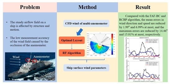
The steady airflow field on a ship is affected by structure and motion and challenged by phenomena such as the low measurement accuracy of the wind field caused by the occlusion of the anemometer. In this work, an improvement in the accuracy of wind measurements affected by structure is proposed, and a method for combining anemometer and X-band marine radar (RCRF) data is designed to further obtain wind parameters. The first step is to use the multivariate bias strategy to achieve the optimal layout of multiple anemometers based on computational fluid dynamics (CFD) numerical simulation data. Then, random forest (RF) is employed to train the wind parameter estimation model. Finally, the wind parameters are optimally estimated by combining the anemometer with the X-band radar. Under the ideal simulation, noise, and temporal uncertainty combined with anemometer noise conditions, the RCRF algorithm performance is evaluated. Compared with the bias correction combination four-anemometer weighted fusion algorithm (FAF-BC) and the BP neural network algorithm for radar wind measurement combination (RCBP), the mean errors in wind direction and speed are reduced by 1.99° and 6.99% at most. The maximum errors are reduced by 14.46° and 15.81% at most, respectively.

1. Introduction

The measurement of ship surface wind parameters $W_{sp}$ is used for ship control, navigation, maritime military operations, and the SHOL envelope establishment of carrier-based aircraft [1,2]. The airflow field usually changes with space and time and changes when passing through the ship and its structure, resulting in an increasing bias in the measured value of the anemometer. In severe cases, this will directly threaten the safety of military activities and military operations [3,4,5]. The traditional measurement method assumes free flow in the arrangement area of the anemometer at the mast. However, with the development of ship technology, more and more large-scale monitoring and investigation equipment is arranged on the ship’s surface, and the damage to this assumption becomes more and more serious [6,7]. As a result, the error in the actual measurement of wind parameters increases and can no longer meet the requirements of the measurement accuracy of wind parameters for sensitive operations such as carrier-based aircraft take-off and landing [8]. The measurement of the ship’s surface wind field is particularly important for ships that provide the take-off and landing of carrier-based aircraft because these operations may be unsafe or impossible to implement under poor wind measurement conditions. Therefore, high-precision wind field measurement is of great significance for ships during offshore operations. The ship’s surface wind parameters $W_{sp}$ are measured directly with an anemometer mounted on the mast, and the sea surface wind parameters $W_{sa}$ are measured by marine radar. Two main aspects of the ship’s surface wind parameters $W_{sp}$ were studied by many researchers: deviation analysis and bias correction [9].

Deviation analysis relies on various methodologies to understand the relationship between anemometer readings and true wind conditions. It encompasses wind tunnel tests [10], computational fluid dynamics (CFD) simulations [11,12,13,14], real sea trials [15], and other experimental techniques. Its primary aim is to identify disparities between the readings and the actual wind, examining the extent to which these variations deviate from the established baseline trend. In a study conducted by Yelland et al. [16], a CFD model was utilized to simulate the airflow around a ship. Anemometers were strategically positioned in exposed and non-exposed areas to capture wind speed measurements. The findings revealed a discrepancy in wind speed readings of approximately 10%. Subsequently, Moat et al. [17,18,19], building upon Yelland’s work, investigated various anemometer placement configurations. Their research highlighted that the correct placement of anemometers reduced distortions in the airflow field. Further investigation by O’Sullivan et al. [20] suggested that discrepancies between measured values and actual wind conditions were potentially influenced by the selection of inappropriate CFD numerical simulation models. They proceeded to compare CFD simulation outcomes with the measured values from the RV Celtic Explorer ship, detecting an error margin of less than 12%. Following the replacement of the CFD numerical simulation model, the accuracy of the simulation results significantly improved by approximately 3% using the Large Eddy Simulation (LES) model [21]. This type of research predominantly focuses on the influence of a ship’s surface structure on measurement discrepancies. It scrutinizes the distortion levels present in the single-point anemometer measurements, which, though informative, are unable to provide a comprehensive understanding of the effective wind parameters.

Bias correction is a vital aspect of wind parameter measurement, necessitating the rectification of biases in ship anemometer measurements [22]. Several methods are employed for this purpose, including the table-check method [23,24], the anemometer bias management (ABM) strategy [15], and the bias correction combination four-anemometer weighted fusion algorithm (FAF-BC) [25]. These studies are designed to mitigate or eliminate deviations between the measured wind parameter values and the actual wind conditions. The table-check method, as investigated by Blanc et al. [26,27], aims to correct the readings of individual anemometers located near the mast and assess its effectiveness, particularly in ideal environmental conditions. Recent research by Polsky et al. [28] revealed that the anemometer mounted on the ship’s mast is significantly affected by mast-induced shelter, as observed during a computational fluid dynamics (CFD) numerical simulation experiment. Consequently, the Anemometer Position Evaluation (APE) strategy was proposed to delineate the range of wind indications suitable for indicating carrier-based aircraft flight operations, effectively reducing anemometer measurement deviations by excluding unsuitable wind indication ranges. Following the APE strategy, Thornhill et al. [15] introduced the ABM strategy, which involves bias correction within the anemometer’s useful angle range to enhance the accuracy of wind parameter measurements on the ship’s surface. To further reduce anemometer measurement deviations, the bias correction links in ABM strategies were used by Zhang et al. [25] to jointly estimate the measured values of the four anemometers with the FAF-BC algorithm. This integrated approach contributes to a more precise correction of anemometer measurement biases. This type of research involves obtaining deviation information through deviation analysis and subsequently rectifying these biases through bias correction techniques. Deviation analysis research primarily concentrates on identifying and pinpointing deviations in wind parameters, whereas bias correction research is geared towards mitigating these biases in wind parameters. Although bias correction methods can yield more accurate wind parameter measurements compared to deviation analysis alone, they currently fall short of fulfilling the requirements for enhancing the precision of wind field measurements.

Marine radar offers the advantage of remotely sensing sea surface wind parameters $W_{sa}$ from a distance of approximately 1 to 2 km from the ship. This method avoids most of the obstruction caused by the ship’s upper structure, and the measured values can be considered as representing undistorted winds at an infinite distance [29,30,31]. The algorithms [32] for small-scale streak retrieval include, but are not limited to, the local gradient method (LGM), the adaptive reduction method (ARM), and the energy spectrum method (ESM). To obtain an image with only wind streaks, the LGM algorithm [33] required the integration, smoothing, and subsampling of the radar image sequence. Then, the LGM algorithm was implemented to determine the gradient direction of the image. To resolve the 180° ambiguity, normalized radar cross-sections (NRCS) were compared to the direction of the sea surface wind $W_{sa}$. In determining the direction of the sea surface wind $W_{sa}$, the ARM algorithm [34] applied an adaptive reduction operator followed by an adaptive local gradient. In the ESM algorithm [35], the sea surface static image was first obtained, and then the small-scale wind streaks were extracted. Finally, more accurate sea surface wind direction parameter information was extracted. The ship’s surface wind field is usually measured by shipborne anemometers. However, the measurement can be significantly affected by obstructions (e.g., mast). There is a noticeable absence of research on applying remote sensing wind direction data for the calibration of ship surface wind fields. The X-band marine radar can measure sea surface wind within a range of approximately 1 to 2 km from the ship. In this study, we propose to employ marine radar-derived wind field parameters to rectify the anemometer’s wind measurements to obtain more precise wind parameters on the ship’s surface.

The CFD numerical simulation technology was used by [25] to obtain the distortion characteristics of the airflow field around the anemometer arrangement area under different speeds. On the basis of correcting the bias of the anemometer, the multi-anemometer measurements were fused and estimated to obtain the only effective wind parameter information. The research showed that the wind measurement error was still too large. In order to meet the strong demand of users for an improvement in accuracy, in this paper, we carry out further research on the basis of [25]. Firstly, a multivariate bias strategy is proposed to optimize the layout of multiple anemometers at the mast. Secondly, the random forest (RF) algorithm is proposed to overcome the limitations of traditional algorithms and accurately express the nonlinear characteristics of the data. Finally, the wind direction parameters of marine radar are introduced to jointly estimate the steady-state wind parameters on the ship’s surface $W_{sp}$.

Regarding studies on wind parameters estimated with multiple anemometers, they are limited to improving the accuracy of wind parameter estimation using only anemometer data. Therefore, it is valuable to combine these data with X-band marine radar to improve the estimation accuracy of wind parameters. In this paper, numerical simulations are used to obtain the anemometer steady-state wind field simulation data on a ship’s surface (Section 2). Then, according to the wind field simulation data, the RCRF algorithm is proposed, and the process of this algorithm is introduced (Section 3). To verify the performance of the algorithm, the estimated wind parameters are compared and analyzed in Section 4. In addition, both the Back Propagation (BP) algorithm and the RF algorithm have never been used for ship surface wind calibration. In this study, both algorithms are employed and compared for ship surface wind correction. Finally, this paper is summarized (Section 5).

2. Model and Data

2.1. Numerical Simulation Physical Model

Information about ocean wind fields is essential for maritime operations and the safe navigation of ships [36]. To obtain the wind direction and speed values of the monitoring points on the ship surface, the CFD calculation software FLUENT 15.0 is used to numerically simulate the steady-state wind field. When modeling the mast structure of the ship, the mast part of the anemometer in the superstructure of the ship is mainly studied; that is, only the physical model of the arrangement position of the shipboard anemometer is considered [25]. In the model, only structures with a great influence on the wind field are selected to facilitate the use of ProE software for modeling, and the mast model needs to be simplified.

The Model-05103 anemometer is used in the numerical simulation modeling process. The wind direction deviation is 3°, and the wind speed deviation is 3 m/s. Because the overall size of the anemometer is very small compared to the mast, it can be ignored in the modeling process. The error of wind speed measured by the combined model of the anemometer and ship structure is slightly larger than that measured by the anemometer alone; the measurement error between the two models is within 3% [8]. Therefore, the anemometer is modeled as a single point in the CFD numerical simulation calculation process.

The CFD numerical simulation is based on the US LHA class ship [8], which reasonably simplifies the physical model (radar, antenna, other ancillary structures, etc.) at the installation position of the anemometer. In the CFD numerical simulation calculation, the flow field calculation area takes 10 times the length of the column platform ground side before the anemometer, 20 times the length of the column platform ground side after the anemometer, 5 times the length of the column platform ground side on both sides, and 5 times the length of the column platform ground side in the vertical direction. The Reynolds order of magnitude, based on the length of the column platform ground side as the characteristic scale, is 1.0 × 10⁷. For the basic boundary conditions of CFD, the position of the entrance in the calculation area of the numerical simulation physical model is relatively far away from the calculation model. Therefore, the inlet boundary condition of the whole model is set as the wind speed inlet, and the outlet boundary condition is set as the pressure outlet. In this paper, the steady-state airflow field on the ship surface is considered a viscous flow. Then, the solid wall boundary condition is set as a non-slip wall, and the other boundaries are set as a free-slip wall. The mast model studied in this paper is relatively simple, so the structural grid mesh ICEM method is used to divide the calculation model [25]. To obtain the multi-anemometer monitoring point simulation database, the grid generated by ICEM software is first imported into FLUENT15.0. Secondly, the SIMPLE algorithm is selected to solve the transport equation of the RNG $k-\epsilon$ model by coupling the pressure field and the velocity field, and the $k$ equation and the $\epsilon$ equation are solved according to the first-order upwind format. The convergence of the residuals, turbulent energy values, and velocity values of each variable is checked to monitor the convergence of the calculation and the minute calculation of the mathematical model reference [8]. Finally, the wind field simulation data under the input condition of a steady-state wind field are obtained.

2.2. Anemometer and Radar Data

In the calculation, the position X = 0.0 m is initially chosen and diffuses outwards from the transverse beam at +3 m and −3 m. On each side, six wind measurement points are selected at a distance of 1 m. In addition, a cross beam is added at X = −4.6 m, so a total of 24 wind measurement points are selected, as shown in

Table 1. Position coordinates of monitoring points.

Monitoring Point	X-Axis	Y-Axis	Z-Axis	Monitoring Point	X-Axis	Y-Axis	Z-Axis
1	0.0 m	−3 m	11.5 m	13	−4.6 m	−3 m	11.5 m
2	0.0 m	−4 m	11.5 m	14	−4.6 m	−4 m	11.5 m
3	0.0 m	−5 m	11.5 m	15	−4.6 m	−5 m	11.5 m
4	0.0 m	−6 m	11.5 m	16	−4.6 m	−6 m	11.5 m
5	0.0 m	−7 m	11.5 m	17	−4.6 m	−7 m	11.5 m
6	0.0 m	−8 m	11.5 m	18	−4.6 m	−8 m	11.5 m
7	0.0 m	3 m	11.5 m	19	−4.6 m	3 m	11.5 m
8	0.0 m	4 m	11.5 m	20	−4.6 m	4 m	11.5 m
9	0.0 m	5 m	11.5 m	21	−4.6 m	5 m	11.5 m
10	0.0 m	6 m	11.5 m	22	−4.6 m	6 m	11.5 m
11	0.0 m	7 m	11.5 m	23	−4.6 m	7 m	11.5 m
12	0.0 m	8 m	11.5 m	24	−4.6 m	8 m	11.5 m

. Initial wind speed is classified into five speed cases (A to E) for the initial free-stream wind field simulation test conditions, ranging from 3 m/s to 15 m/s (each increasing by 3 m/s). For each speed case, 72 wind angles (increasing every 5° from 0° to 360°) are selected as the initial wind direction. The 24 wind monitoring points are used to simulate the wind parameters on the ship’s surface $W_{sp}$ in this paper, for a total of 8640 sets of wind field numerical simulation data under the steady wind input condition. Data from all wind monitoring points are divided into 360 groups, each of which contains a pair of wind direction and wind speed values.

The marine radar data used in this work are derived from the marine radar of the wave monitoring equipment experimental platform. The marine radar collected a large amount of data on the open sea of the Pingtan Marine Environmental Monitoring Station of the State Oceanic Administration from October to November 2010. The wind speed is 15.3~19.1 m/s, the wave direction is 102°~105°, and the wave height is 1.3~5.8 m. The wave near the experimental platform is dominated by wind waves, and the wave direction is basically the same as the wind direction [37]. The parameters of the X-band marine radar are shown in

Table 2. X-band marine radar parameters.

Radar Parameters	Performance
Electromagnetic Wave Frequency	9410 $\pm$ 30 MHz
Antenna Angular Speed	${26}_{-6}^{+2}$ r.p.m
Antenna Height	25 m
Polarization	HH
Horizontal Beam Width	≤$1.3°$
Vertical Beam Width	$23°\pm 2°$
Range Resolution	7.5 m
Pulse Repetition Frequency	Short Pulse: $1300\pm 10\mathrm{\%}$ Hz
Pulse Width	$0.7°$
RF Pulse Envelope Width	${0.05}_{-0.02}^{+0.03} \mathsf{\mu }\mathrm{s}$
RF Pulse Peak Power	Short Pulse: $\ge 16 \mathrm{K}$W
Receiver IF Bandwidth	Short Pulse: $20\pm 3 \mathrm{M}$Hz
Azimuth Resolution	1.8 m Antenna: $\le 1.3°$

. The rotation time of the radar antenna is 2.5 s. The number of lines generated by a single radar image is 2048, and the number of pixels for each line is 600.

3. Method

The anemometer at the mast of the actual ship surface is often blocked by the surrounding structure, which makes the anemometer unable to accurately measure the undistorted wind [31]. At the mast, each anemometer is affected by the airflow distortion phenomenon at different undistorted relative wind angles. For the anemometer with poor exposure conditions, the wind direction deviation is up to 22%, and the wind speed deviation is up to approximately 25% [15]. Usually, there are two or more anemometers arranged at the mast of a ship. The traditional wind parameter measurement method [8] selects the anemometer measurement value with the largest measured wind speed as the final wind parameter output. This method requires that the airflow field in the mast anemometer arrangement area is not disturbed by the hull structure. Therefore, when the airflow field in the mast anemometer layout area tends to be stable, the method is effective and can be used as a source of verification data for wind retrieved by radar images. However, when the ship mast anemometer is in a complex arrangement position, the center diameter of the ship, especially the military ship mast, is larger than that of other types of ships, and the shielding range of the anemometer is increased, resulting in a large error in the wind parameter measurement value output by the traditional method. However, the X-band marine radar can effectively compensate for the error caused by the anemometer wind measurement due to its advantage of not being occluded in the measurement area [38,39]. Therefore, the retrieved theory of the sea surface wind parameters $W_{sa}$ of X-band marine radar and the strong nonlinear mapping characteristics of the random forest (RF) algorithm are used, and the RCRF algorithm is proposed in this paper. The structure flow of this algorithm is shown in Figure 1.

The focus of this study is slightly different from the FAF-BC algorithm [25]. Firstly, a multivariate bias strategy is proposed to study the optimal layout of multiple anemometers at the mast. In practical engineering applications, when there are multiple anemometers on the ship’s surface, the arrangement position of the anemometers is often obscured by the surrounding structures, resulting in inaccurate measurement values. With the continuous updating and upgrading of the ship structure, more and more equipment is installed near the mast, which leads to the problem of a large error between the measured value of the anemometer and the free airflow at infinity. Therefore, addressing the multi-anemometer layout problem is the first step towards solving the problem of a large error between the measured value and the free airflow at infinity and provides an effective measurement value for the subsequent multi-anemometer estimation problem. Secondly, it is worth noting that the application of machine learning algorithms such as BP, support vector machine (SVM), and RF is becoming more and more extensive. The RF algorithm belongs to the ensemble learning family, combining multiple weak classifiers to achieve a better ensemble classifier. Due to the nonlinear characteristics of the data, the RF has good robustness to noise and missing data, and the training speed is relatively fast when dealing with large datasets. Another trend is to combine previous physical knowledge with machine learning models to overcome the limitations of traditional methods, which often fail to accurately obtain the complex relationships between wind parameters. Finally, people are becoming more and more interested in machine learning models. Accurate and reliable prediction is crucial for carrier-based aircraft pilots to make decisions. Thirdly, the airflow field changes with space and time in the real environment, and the anemometer at the mast produces a turbulence effect when measuring the wind parameters. The X-band marine radar can filter out the random turbulence generated by the wind field through its low-pass filtering. On the other hand, the measurement of the anemometer at the mast is easily affected by the occlusion of the structure and the steering of the ship. The airflow field around the anemometer is unstable and disturbed, such that there is a large error between the wind parameters measured by the anemometer and the free airflow wind parameters. The marine radar has the advantage of remotely sensing the sea surface wind field information at a distance of 1 km from the ship, avoiding the occlusion of the upper structure of the ship, and the measured value can be approximated as the free airflow at infinity. Therefore, the combination of the measured values of the marine radar and the anemometer can theoretically avoid the problem of a large error in the measured values when the ship mast anemometer is in a complex arrangement position and can improve the estimation accuracy of the steady-state wind parameters on the ship’s surface $W_{sp}$.

3.1. Simulating Anemometer Wind Data

3.1.1. Optimal Layout of Multiple Anemometers Based on Multivariate Bias Strategy

Usually, anemometers are arranged on the left and right sides of the central mast of the bridge to monitor the wind field on the ship’s surface in real time, and the method of employing angle bias and speed bias [15] is widely used to study the layout of the dual anemometers. However, wind in nature is composed of wind speed and wind direction; that is, the wind field is a vector. The wind field data measured by the anemometer at any time include two inseparable parts: wind speed and wind direction. The process of using the angle bias and speed bias to evaluate the measured wind direction and wind speed, respectively, may cause a large bias of the measured wind speed at a certain moment, but the bias of the measured wind direction is small. It may also cause a small bias of the measured wind speed at a certain moment, but the bias of the measured wind direction is very large. This will lead to an inability to understand the true biases of the wind vector measured at each moment.

At present, most researchers are focused on the optimal layout method of dual anemometers, but there are relatively few studies on the optimal layout method of multiple anemometers. In practical engineering, the layout of multiple anemometers can better monitor the wind parameters of airflow at infinity at different angles. Therefore, to obtain more comprehensive and accurate wind parameter information in a given arrangement position, an optimal layout method for multiple anemometers based on the multivariate bias strategy is constructed. The multivariate bias method is used as the index to judge the wind parameter error, and the optimal arrangement scheme of the multiple anemometers is determined by analyzing the error results. The flow chart is shown in Figure 2.

The 24 wind monitoring points calculated in Table 1 are used as the wind field information of the primary selection monitoring points, and the number of monitoring points ranges from 2 to 24. Because the dimension of angle bias is given in degrees, and the speed bias has no dimension, the first evaluation index of multivariate bias is proposed: the relative bias of wind parameters. It is defined as the sum of the relative error of angle bias and the relative error of speed bias.

$${\gamma }_W={\overline{\gamma }}_{W_{\theta }}+{\overline{\gamma }}_{W_v},$$

(1)

$${\overline{\gamma }}_{W_{\theta }}=\left|\frac{{\beta }_{\theta }}{{\theta }_I}\right|\times 100\%,$$

(2)

$${\overline{\gamma }}_{W_v}=|{\beta }_v-1|\times 100\%,$$

(3)

where ${\gamma }_W$ is the relative bias of wind parameters; ${\overline{\gamma }}_{W_{\theta }}$ is the relative error of angle bias; ${\overline{\gamma }}_{W_v}$ is the relative error of speed bias; ${\beta }_{\theta }$ is the angle bias, which is defined as the difference between the measured wind direction and the initial wind direction; ${\beta }_v$ is the speed bias, which is defined as the ratio between the measured wind speed and the initial wind speed; and ${\theta }_I$ is the initial wind direction. When the wind parameter bias is smaller, the accuracy of the measured wind field is higher; otherwise, the accuracy of the measured wind field is lower. In addition, the second evaluation index of multivariate bias is proposed: wind vector difference. This represents the vector error between the initial wind parameters and the measured wind parameters. The larger the wind vector differential mode, the larger the error between the initial wind parameters and the measured wind parameters. The wind vector difference includes not only the relationship between the initial wind speed and the measured wind speed but also the relationship with wind direction. The wind field error vector diagram is shown in Figure 3.

${\overrightarrow{V}}_I$ is the initial wind speed vector; ${\overrightarrow{V}}_M$ is the measured wind speed vector; ${\theta }_I$ is the initial wind direction; ${\theta }_M$ is the measured wind direction; and ${\overrightarrow{V}}_{WVD}$ is the wind vector difference. Then, the wind vector difference is

$$\begin{gathered} {\overrightarrow{V}}_{WVD}={\overrightarrow{V}}_I-{\overrightarrow{V}}_M \\ =({\overrightarrow{e}}_x\left|{\overrightarrow{V}}_I\right|{\mathit{sin}\theta }_I+{\overrightarrow{e}}_y\left|{\overrightarrow{V}}_I\right|{\mathit{cos}\theta }_I)-({\overrightarrow{e}}_x\left|{\overrightarrow{V}}_M\right|{\mathit{sin}\theta }_M+{\overrightarrow{e}}_y\left|{\overrightarrow{V}}_M\right|{\mathit{cos}\theta }_M) \\ ={\overrightarrow{e}}_x(\left|{\overrightarrow{V}}_I\right|{\mathit{sin}\theta }_I-\left|{\overrightarrow{V}}_M\right|{\mathit{sin}\theta }_M)+{\overrightarrow{e}}_y(\left|{\overrightarrow{V}}_I\right|{\mathit{cos}\theta }_I-\left|{\overrightarrow{V}}_M\right|{\mathit{cos}\theta }_M), \end{gathered}$$

(4)

where ${\overrightarrow{e}}_x$ and ${\overrightarrow{e}}_y$ are unit vectors of the X and Y axes. The relative errors of wind vector differential mode ${\delta }_i$ and wind vector differential mode $\left|{\overrightarrow{V}}_{WVD}\right|$ are

$$\left|{\overrightarrow{V}}_{WVD}\right|=\sqrt{(\left|{\overrightarrow{V}}_I\right|{\mathit{sin}\theta }_I-\left|{\overrightarrow{V}}_M\right|{\mathit{sin}\theta }_M{)}^2+(\left|{\overrightarrow{V}}_I\right|{\mathit{cos}\theta }_I-\left|{\overrightarrow{V}}_M\right|{\mathit{cos}\theta }_M{)}^2},$$

(5)

$${\delta }_i={\left|{\overrightarrow{V}}_{WVD}\right|}_i/{\left|{\overrightarrow{V}}_I\right|}_i\cdot 100\%,$$

(6)

Since there are 72 sets of wind field data under each speed case, the wind field data under each speed case are averaged. Finally, the relative biases of the wind parameters and wind vector difference are fused:

$$D_M=\raisebox{1ex}{$\left(\sum _{i=1}^{72}{\delta }_i\right)$}\!\left/ \!\raisebox{-1ex}{$72$}\right.+\raisebox{1ex}{$\left(\sum _{i=1}^{72}{\gamma }_{Wi}\right)$}\!\left/ \!\raisebox{-1ex}{$72$}\right.,$$

(7)

where $D_M$ is the multivariate bias value, and ${\gamma }_{Wi}$ is the $i-th$ relative bias of the wind parameters.

3.1.2. Random Forest (RF)-Based Wind Parameter Estimation Algorithm

In 2001, Breiman Leo and Adele Cutler [40] proposed that random forest is an ensemble learning algorithm. The algorithm contains two key parameters: the number of decision trees and the input characteristics of a single decision tree. The voting of multiple decision trees is used to solve classification and prediction questions in the RF algorithm [41]. In practice, the measured data volume of the anemometer is small, the data randomness is strong, the data are greatly affected by noise, and there are some missing cases. Compared with other machine learning algorithms or boosting tree methods [42], the RF algorithm has a relatively good prediction effect when training small-scale data. This is because each decision tree is trained independently and can be calculated in parallel, and it also has certain advantages in large-scale calculation. Due to the introduction of two sources of randomness in the training process, the RF algorithm is not easy to over-fit and has good anti-noise ability. Moreover, for such data with partial loss, high accuracy can still be maintained. The learning process of the algorithm is relatively fast. The RF algorithm is insensitive to multivariate collinearity, and the results are more robust to missing data and unbalanced data. Therefore, the RF model is designed to estimate the wind parameters of the different multi-anemometer layout schemes on the ship. The principles of random forest are as follows:

• Data selection: The initial wind speed and wind direction are taken as the input (wind direction is initially every 5° interval, and the wind speed is initially 3 m/s, 6 m/s, 9 m/s, 12 m/s, or 15 m/s). Additionally, the CFD wind direction ${\overline{\theta }}_{CFD}$ and CFD wind speed ${\overline{v}}_{CFD}$ measurements under the optimal layout at four different positions are taken as input samples in the training process. Using random sampling and feature selection, the samples are inputted into the RF algorithm to predict wind speed and wind direction. The resulting predictions are referred to as RF wind direction ${\widehat{\theta }}_{RF}$ and RF wind speed ${\widehat{v}}_{RF}$. There are 365 sets of data in the CFD wind database, 80% of which are selected as training data and 20% as testing data;
• Constructing the random forest: The bootstrap method [43] is used to sample the training data 292 times randomly with return sampling. Some data may be selected multiple times due to the replacement extraction, and some data may not be selected. The samples taken out each time are not exactly the same, and these samples constitute the training data set of the decision tree ${\theta }_1$. This operation is repeated to generate the training set ${\theta }_1,{\theta }_2,\dots ,{\theta }_T$, so as to generate $\mathrm{T}$ decision trees for the construction of the random forest model;
• Feature selection: The CFD wind direction and CFD wind speed at four positions of the anemometer are used as the features of the sample data, so the sample data have eight features. In each decision tree node split, the RF randomly selects $k(k\le 8)$ features from all the features with each feature without return. Three features are selected in this paper, and the best segmentation attributes are selected as nodes to build multiple classification and regression trees (CART). The size of $k$ during the growth of the decision tree is always the same;
• Parameter initialization: The number of decision trees ranges from 1 to 292, and the number of decision trees increases by 10 per round of training. The minimum number of leaves is increased by 1 per training from 1. The training method is regression, and the expected error is set to 1 × 10⁻⁵;
• Model training: The multiple decision trees established above form a forest. For each decision tree, the above-selected samples and features are used for training. Figure 4 is the training process structure diagram;
• Results prediction: Similarly, the bootstrap method is also used to generate the testing set ${\theta }_1$ by performing 73 times randomly with return sampling on the testing sample data. After repeating this operation, the testing set ${\theta }_1,{\theta }_2,\dots ,{\theta }_M,M=73$ is generated. The information on the anemometer parameters at different positions studied in this paper is estimated as a regression problem. Therefore, based on the idea of ensemble learning, the mean value of each regression tree is taken as the prediction result. The formula is as follows:

  $$\overline{h}\left(x\right)=\frac{1}{T}{\sum }_{t=1}^T\left\{h\left(x,{\theta }_t\right)\right\},$$

  (8)

  where $\overline{h}\left(x\right)$ is the model prediction result; $h\left(x,{\theta }_t\right)$ is output based on $x$ and ${\theta }_t$; $x$ is the independent variable; ${\theta }_t$ is an independent and identically distributed random vector; and $T$ is the number of regression decision trees. Figure 5 shows the testing process structure diagram.
• Model evaluation: Comparing the testing set error results of different decision tree numbers and leaf numbers, the optimal RF wind parameters are output when the error reaches the expected value. Figure 6 shows the flow chart of RF model training.

In this model, the number of decision trees is set to 200, the minimum number of leaves is set to 2, and the prediction method is set to regression. The training error reaches the expected value when 20 decision trees are trained. At this time, the error of the sample is as low as 5.7264 × 10⁻⁶, and the correlation coefficient calculated by the two samples is greater than 0.99. The error value of the training set is 0.105, and the error value of the test set is 0.138. The error value of the two datasets is small, so this training model does not produce an over-fitting phenomenon, and the fitting effect is very good, as shown in Figure 7 and Figure 8.

3.2. Radar Wind Direction Retrieval

In this paper, the energy spectrum method (ESM) [35] wind direction retrieval algorithm is used to obtain high-precision direction parameters. To reduce the influence of co-frequency interference on the analysis of the sea surface wind field, a 2D nonlinear smoothing median filter with a $3\times 3$ template is applied to the measured radar images.

$$f^{\prime }\left(r,\theta \right)=\underset{\left(s,t\right)\in N\left(r,\theta \right)}{median}\left\{g\left(s,t\right)\right\},$$

(9)

where $g\left(s,t\right)$ is the image echo intensity value of the radar image pixel point at the polar coordinate position $\left(s,t\right)$; $f^{\prime }\left(r,\theta \right)$ is the gray value of the filtered image in the polar coordinate position $\left(r,\theta \right)$; $N\left(r,\theta \right)$ is the pixel point of the center point at $\left(r,\theta \right)$; and $\left(s,t\right)$ takes eight points centered on $\left(r,\theta \right)$. The template center of the $3\times 3$ template median filter is overlapped with the pixel position of the polar coordinate image, and the template traverses the full radar image to obtain the median filtered image sequence, as shown in Figure 9.

The color bar represents the 13-bit pixel intensity; red means the highest pixel intensity, and blue means the lowest pixel intensity. Figure 9 is a polar coordinate image. The range of ρ is 0 to 2500 m, and the range of θ is 0 to 360°. Then, a new polar coordinate image is established to obtain a normalized new polar coordinate image. Based on the characteristics of the static frequency of sea surface wind streaks, the normalized radar image sequence is integrated and averaged at the pixel points at the same position according to the specified compensation time.

$$f\left(\theta ,r\right)=\frac{{\sum }_{t=0}^{N_t}{f}^{\prime }\left(\theta ,r,t\right)}{N_t},$$

(10)

where $f\left(\theta ,r\right)$ is the wind streaks image; $f^{\prime }\left(\theta ,r,t\right)$ is the single radar image of the radar image sequence time $t$; and $N_t$ is the time series. The gray value of the new pixel after low-pass filtering is assigned to the newly constructed two-dimensional polar coordinate image according to the position, and the two-dimensional polar coordinate sea surface static feature image is obtained.

The two-dimensional polar coordinate image is divided into small regions, and the polar coordinates of each small region are interpolated into the established Cartesian coordinates by using the nearest point. The two-dimensional image is then transformed into a two-dimensional discrete fast Fourier transform (2D-FFT) to obtain the energy spectrum of the sea surface static feature image.

$$F\left(k_x,k_y\right)=\sum x_{N_x}\sum y_{N_y}f\left(x_{N_x},y_{N_y}\right)\mathit{exp}\left[-i \ast 2\pi \left(\frac{x_{N_x} \ast k_x}{\mathit{max}\left(x_{N_x}\right)}+\frac{y_{N_y} \ast k_y}{\mathit{max}\left(y_{N_y}\right)}\right)\right],$$

(11)

where $F\left(k_x,k_y\right)$ is the Fourier coefficient of the sea surface static feature image; $x_{N_x}$ and $y_{N_y}$ are the number of pixels of $x$ and $y$ axes in the spatial domain of sea surface static feature image in Cartesian coordinates. Wavenumber energy spectrum scale separation is applied to the energy spectrum of static feature images. The upper and lower limits of the wind streak energy spectrum beam are calculated according to the relationship between the wind streak wavelength $L$ and the frequency domain coordinate scale $k$. The wind streak signal energy spectrum is extracted using the energy spectrum bandpass filter. The mathematical model is

$$I\left(k_x,k_y\right)=\left\{\begin{array}{c}A\left(k_x,k_y\right)\left(\sqrt{k_x^2+k_y^2}\in \left[\left|k_d\right|,\left|k_t\right|\right]\right)\\ 0 \left(else\right)\end{array}\right.,$$

(12)

where $I\left(k_x,k_y\right)$ represents the energy spectrum of wind streaks. Figure 10 is the energy spectrum of the wind streak contour obtained by $I\left(k_x,k_y\right)$ in $\left(k_x,k_y\right)$ coordinates after wavenumber scale separation. The imaginary line is the wavelength range in $\left(k_x,k_y\right)$ coordinates.

In Figure 10, $k_x$ and $k_y$ represent the horizontal and vertical coordinates of the beam domain. The energy concentration area is the red area, the yellow area is the area with higher energy, and the blue area is the area with lower energy. The direction of the line connecting the two energy concentration areas is the vertical direction of the wind streak and the north-facing sea surface wind direction $N_w^i(i=\mathrm{1,2},3,\dots )$ of each subregion can be obtained. The main wind direction ${\theta }_{radar}$ of the sea surface can be determined as follows:

$${\theta }_{radar}={\sum }_i{N}_W^i(i=\mathrm{1,2},3\dots ,14),$$

(13)

3.3. Combining Anemometer and Radar Results

The RF wind direction ${\widehat{\theta }}_{RF}$ is constrained by the measurement data of the wind direction ${\theta }_{radar}$ retrieved from the marine radar image. Since the wind direction obtained by the ESM algorithm has a standard deviation $\sigma$ of 8.29°, it can be assumed that the wind direction measured by the radar has an uncertainty of $\pm 20^{°}(<3\sigma )$. Therefore, in the range ${\theta }_{radar}\pm 20^{\circ }$ of the wind direction constraint angle measured by radar, the output of the RF wind direction in this range is divided into one group every 5° for $j$ groups in total.

In the range of ${\theta }_{radar}\pm 20^{\circ }$, the cost function of each group of RF wind direction ${\widehat{\theta }}_{RF,j}$ and radar-measured wind direction ${\theta }_{radar}$ are calculated.

$$\mathit{min}J\left(\theta \right)={‖{\theta }_{\mathit{radar}}-{\widehat{\theta }}_{\mathit{RF},j}‖}_{-\infty }=min\left|{\theta }_{radar}-{\widehat{\theta }}_{RF,j}\right|,$$

(14)

where ${\widehat{\theta }}_{RF,j}$ is the j-th group of the RF wind direction; ${‖·‖}_{-\infty } \mathrm{i}\mathrm{s}-\infty \mathrm{n}\mathrm{o}\mathrm{r}\mathrm{m}$. In this paper, in the range of ${\theta }_{radar}\pm 20^{\circ }$, the pair of estimates with the smallest cost function in the group is taken as the optimal wind parameters estimation output of the RCRF algorithm.

4. Results

4.1. Performance Evaluation Index

The anemometer produces a range of noise in the real environment, including electromagnetic radiation, thermal noise, shot noise, and other internal noise generated by the sensor circuit components [44,45]. As a result, the anemometer itself also generates a systematic measurement error. To bring the verification data closer to the measurement results of the anemometer in the actual environment, it is necessary to introduce the anemometer error itself into the CFD wind field simulation data. The anemometer measurement error and the CFD wind data are taken as the wind field verification data, as shown in the following equation:

$$\widehat{X}={\widehat{X}}_f+N\left(0,{\sigma }^2\right),$$

(15)

where $\widehat{X}$ represents the wind field verification data; ${\widehat{X}}_f$ represents the CFD wind data; $N(0,{\sigma }^2)$ represents the anemometer measurement error, the mean value is zero, and ${\sigma }^2$ represents the variance.

A Model-05103 anemometer is mounted on either side of the ship mast;

Table 3. Model-05103 anemometer technical specifications.

Measuring Parameters	Measuring Range	Measurement Accuracy	Resolving Power
Wind Direction	0~360°	±3°	1°
Wind Speed	0~60 m/s	±0.3 m/s	0.1 m/s

lists key specifications. The direction and speed measurement errors are 3° and 0.3 m/s, respectively. Consequently, a wind direction error of 0 and a variance of 9, as well as a wind speed error of 0 and a variance of 0.09, are added to the CFD wind data. In the subsequent test analysis, the marine radar data and the anemometer data are both simulated data under ideal environmental conditions, and the environmental conditions and parameters are the same. The performance of the RCRF algorithm is verified using the wind field measurement data with ideal simulation, anemometer noise, and temporal uncertainty combined with anemometer noise [25].

To evaluate the influence of this method on the wind parameter estimation, the results of the FAF-BC algorithm and the radar wind measurement combined with the BP neural network algorithm (RCBP) [46,47] are compared. The RCBP algorithm has been used in previous research, and the BP algorithm is used to estimate the steady-state wind parameters of the ship. However, due to the limitations of BP itself, it is used as a comparison algorithm. The difference between the implementation processes of the RCBP method and the RCRF method is that the machine learning algorithm is different, and the implementation process of other methods is the same. The absolute error index of wind direction ${MAE}_{\theta }$ and the relative error index of wind speed ${MRE}_v$ are chosen as the indexes for evaluating the algorithm performance in this study.

$${MAE}_{\theta }=\left|{\theta }_{RCRF}-{\theta }_I\right|,$$

(16)

$${MRE}_v=\left|\frac{{\nu }_{RCRF}-{\nu }_I}{{\nu }_I}\right|,$$

(17)

where ${\theta }_{RCRF}$ is the optimal direction estimate; ${\theta }_I$ is the initial wind direction; ${\nu }_{RCRF}$ is the optimal speed estimate; and ${\nu }_I$ is the initial wind speed.

4.2. Quantitative Evaluation under Ideal Condition

Under the ideal simulation conditions, Figure 11 shows the performance analysis and comparison of FAF-BC, the RCBP algorithm, and the RCRF algorithm in five speed cases (speed cases A through E; the standard wind speeds are 3, 6, 9, 12, and 15 m/s).

For the speed error values, Figure 11a gives the ${MRE}_v$ of the FAF-BC algorithm. In the range of 0° to 180° of the undistorted relative wind angles, most of the ${MRE}_{v}s$ are distributed between 3% and 10%, a small part of the ${MRE}_v\mathrm{s}$ are distributed over 10%, and the maximum ${MRE}_v$ is about 17%. In addition, under different wind speed cases, the ${MRE}_v$ trend of the algorithm is consistent. The ${MRE}_v$ of the RCBP algorithm is displayed in Figure 11b. Most of the ${MRE}_{v}s$ are distributed between 2% and 6% in the 0° to 180° range of the undistorted relative wind angles. A small part of the error values are distributed over 6%, and the maximum ${MRE}_v$ is about 9.3%. Additionally, the ${MRE}_v$ trend of the RCBP algorithm is generally consistent under different speed cases. For undistorted relative wind angles in the range of 0° to 90°, the ${MRE}_v$ law shows a more obvious discrete trend, while in the range of 90° to 180°, the discrete trend of this law gradually weakens. The ${MRE}_v$ of the RCRF algorithm is illustrated in Figure 11c, in which the ${MRE}_v$ is below 2%, and the maximum ${MRE}_v$ is about 1.8%. However, under different speed cases, the ${MRE}_v$ trend of the RCRF algorithm has no obvious law, which may be caused by the randomness of this algorithm.

For the direction error value, Figure 11d is the ${MAE}_{\theta }$ of the FAF-BC algorithm. It can be observed that the ${MAE}_{\theta }$ in most of the undistorted relative wind angles is below 3°. In addition, under different wind speed cases, the ${MAE}_{\theta }$ of the FAF-BC algorithm also maintains a good consistency. The ${MAE}_{\theta }$ of the RCBP algorithm is shown in Figure 11e. The error value is large only for undistorted relative wind angles in the range of 30° to 80°, and the error value is below 2° at other angles (except for the odd values). Similarly, under different speed cases, the discrete trend of the ${MAE}_{\theta }$ law in the range of 90° to 180° is weakened. Otherwise, the odd value is caused by the random error in the CFD simulation process, and the data quality of the odd value is controlled in the subsequent calculation process. The ${MAE}_{\theta }$ of the RCRF method is displayed in Figure 11f; it can be observed that the ${MAE}_{\theta }$ for most of the undistorted relative wind angles is distributed below 0.5° (except for the odd values). In addition, under different speed cases, the ${MAE}_{\theta }$ of the RCRF algorithm also maintains a good consistency. To compare the performance of the three algorithms, the ${MRE}_v$ and ${MAE}_{\theta }$ of the three algorithms under case E are compared, as shown in Figure 12.

Figure 12 presents a comparison diagram of the ${MRE}_v$ and ${MAE}_{\theta }$ of the three algorithms under ideal conditions. The red square line represents the ${MRE}_v$ of the R-IFAF-BC algorithm, the blue circle line represents the ${MRE}_v$ of the RCRF algorithm, and the black star line represents the ${MRE}_v$ of the FAF-BC algorithm. Figure 12a shows the ${MRE}_v$ comparison diagram. It can be observed that the error value distribution of most RCRF algorithms is lower than that of the FAF-BC and RCBP algorithms. Figure 12b shows the ${MAE}_{\theta }$ comparison diagram. Similarly, the error value distribution of most RCRF algorithms is lower than that of the FAF-BC and RFBP algorithms.

Based on ideal simulation conditions, the maximum and mean errors of both algorithms are compared, as shown in

Table 4. Maximum and mean error comparison of three algorithms under the ideal conditions.

Condition	Method	Mean Error		Maximum Error
		MRE (%)	MAE (°)	MRE (%)	MAE (°)
Ideal condition	FAF-BC algorithm	5.30	1.29	−16.98~+8.37	−6.11~+2.57
	RCBP algorithm	2.36	0.85	−9.26~+4.60	−2.52~+2.52
	RCRF algorithm	0.13	0.11	−1.17~+1.67	−3.15~+1.85

. Regarding the speed error value, compared with the FAF-BC algorithm, the mean ${MRE}_v$ of the RCRF algorithm is improved by 5.17%, the minimum value is reduced by 15.81%, and the maximum value is decreased by 6.70%. Compared with the RCBP algorithm, the mean ${MRE}_v$ of the RCRF algorithm is enhanced by 2.23%, the minimum value is reduced by 8.09%, and the maximum value is decreased by 2.93%. Regarding the wind direction error value, the mean ${MAE}_{\theta }$ of the FAF-BC algorithm is reduced by 1.18°, the minimum value is increased by 2.96°, and the maximum value is decreased by 0.72°. The ${MAE}_{\theta }$ mean of the RCRF algorithm is reduced by 0.74°, the minimum value is increased by 0.63°, and the maximum value is decreased by 0.67°. Therefore, under the ideal simulation conditions, the RCRF algorithm can effectively improve the estimation accuracy of wind parameters.

4.3. Quantitative Evaluation under Noise Condition

Under the condition of introducing the measurement error of the anemometer itself, the performance analysis and comparison of the FAF-BC algorithm, RCBP algorithm, and RCRF algorithm are displayed in Figure 13.

For the speed error value, Figure 13a shows the ${MRE}_v$ of the FAF-BC algorithm. In the range of 0° to 180° of the undistorted relative wind angles, most of the ${MRE}_{v}s$ are distributed between 3% and 10%, a small part of the error values are distributed over 10%, and the maximum ${MRE}_v$ is about 16%. In addition, under different speed cases, the ${MRE}_v$ of the FAF-BC algorithm shows a discrete trend due to the introduction of anemometer noise. The ${MRE}_v$ of the RCBP algorithm is demonstrated in Figure 13b. Most of the ${MRE}_{v}s$ are distributed between 2% and 6% for undistorted relative wind angles in the range of 0° to 180°, a small part of the $MREs$ are distributed over 6%, and the maximum ${MRE}_v$ is about 9%. In addition, under different speed cases, the ${MRE}_v$ of the RCBP algorithm shows a discrete trend due to the introduction of anemometer noise. The ${MRE}_v$ of the RCRF algorithm is illustrated in Figure 13c, in which the ${MRE}_{v}s$ are almost all distributed below 1%, and the maximum ${MRE}_v$ is about 4%. However, under different speed cases, the ${MRE}_v$ of the RCRF algorithm also displays the same discrete trend due to the addition of noise, but the trend is weaker.

For the direction error value, the ${MAE}_{\theta }$ of the FAF-BC algorithm is shown in Figure 13d. It can be observed that the ${MAE}_{\theta }$ in most of the undistorted relative wind angles are distributed below 3°. In addition, under different speed cases, the ${MAE}_{\theta }$ of the FAF-BC algorithm is generally consistent (except for the odd value). The ${MAE}_{\theta }$ of the RCBP algorithm is shown in Figure 13e. It can be seen that the ${MAE}_{\theta }s$ in the figure are distributed below 2° for most of the undistorted relative wind angles. Additionally, under different speed cases, the ${MAE}_{\theta }$ law still maintains good consistency. Figure 13f demonstrates the ${MAE}_{\theta }$ of the RCRF algorithm, and most of the ${MAE}_{\theta }s$ in the range of undistorted relative wind angles are below 1° (excluding the odd value). Similarly, under different speed cases, the consistency of the wind direction error law is weak. To compare the performance of the three algorithms, the ${MRE}_v$ and ${MAE}_{\theta }$ of the three algorithms under case E are compared, as shown in Figure 14.

Figure 14 gives a comparison diagram of the ${MRE}_v$ and ${MAE}_{\theta }$ of the three algorithms under noise conditions. Figure 14a shows the ${MRE}_v$ comparison diagram. It can be clearly seen that the error value distribution of most RCRF algorithms is lower than that of the FAF-BC and RCBP algorithms. Figure 14b shows the ${MAE}_{\theta }$ comparison diagram. The error value distribution of the RCRF algorithm is better than that of the FAF-BC and RCBP algorithms. The odd values of the three algorithms for undistorted relative wind angles in the range of 120° to 150° are caused by the simulation error.

Table 5. Maximum and mean error comparison of three algorithms under the noise condition.

Condition	Method	Mean Error		Maximum Error
		MRE (%)	MAE (°)	MRE (%)	MAE (°)
Noise condition	FAF-BC algorithm	6.27	1.72	−16.02~+14.11	−4.23~+4.75
	RCBP algorithm	2.62	1.34	−8.63~+5.74	−2.53~+2.74
	RCRF algorithm	0.18	0.13	−1.67~+4.25	−2.24~+0.53

indicates the comparison of the maximum and mean error values of the two algorithms under the noise condition. For the speed error value, the mean ${MRE}_v$ in the RCRF algorithm compared with the FAF-BC algorithm is enhanced by 6.09% overall, while the minimum is reduced by 14.35% and the maximum is decreased by 9.86%. The mean ${MRE}_v$ in the RCRF algorithm, compared with the RCBP algorithm, is enhanced by 2.44% overall, while the minimum is reduced by 6.96% and the maximum is decreased by 1.49%. For the direction error value, the mean ${MAE}_{\theta }$ in the RCRF algorithm compared with the FAF-BC algorithm is improved by 1.59°, the minimum value reduced by 1.99°, and the maximum value is improved by 4.22°. The mean ${MAE}_{\theta }$ in the RCRF algorithm compared with RCBP algorithm is improved by 1.21°, the minimum value is reduced by 0.29°, and the maximum value is improved by 2.21°. It can be concluded that the RCRF algorithm has a relatively small improvement effect on the mean ${MAE}_{\theta }$, but the effect of the maximum error is improved greatly. Moreover, this algorithm not only effectively reduces the mean ${MRE}_v$ in the RCBP algorithm, but also significantly decreases the maximum error value. Therefore, the RCRF algorithm has a better anti-noise effect in the noise condition, which improves the estimation accuracy of wind parameters to a certain extent.

4.4. Quantitative Evaluation under Temporal Uncertainty Combined with Noise Condition

Under the condition of introducing temporal uncertainty combined with noise, Figure 15 displays the performance analysis and comparison of the FAF-BC algorithm, RCBP algorithm, and RCRF algorithm.

For the speed error value, the ${MRE}_v$ of the FAF-BC algorithm is demonstrated in Figure 15a. The observation shows that the ${MRE}_v$ maximum appears in the range of 60° to 90° with regard to the undistorted relative wind angle, and the ${MRE}_v$ minimum appears when the undistorted relative wind angle is 55°. However, the ${MRE}_v$ under different speed cases has a weak vibration effect with the addition of noise. The ${MRE}_v$ of the RCBP algorithm is demonstrated in Figure 15b. Most of the ${MRE}_{v}s$ are distributed below 8% in the range of undistorted relative wind angles from 0° to 180°, while a small portion of the ${MRE}_{v}s$ are distributed above 10%, with a maximum ${MRE}_v$ of about 13%. In addition, the ${MRE}_v$ of the RCBP algorithm under different speed cases display a substantial discrete trend due to the introduction of the temporal uncertainty combined with the anemometer noise. The ${MRE}_v$ of the RCRF algorithm is illustrated in Figure 15c, in which the ${MRE}_{v}s$ are almost all distributed below 2%, with only one single point error value exceeding 2%, and the maximum ${MRE}_v$ is about 2.2%. Under different speed cases, the ${MRE}_v$ of the RCRF algorithm also demonstrates the same discrete trend under the condition of temporal uncertainty combined with the noise. However, this trend is weak due to the strong anti-noise ability of the RCRF algorithm.

For the direction error value, the ${MAE}_{\theta }$ of the FAF-BC algorithm is shown in Figure 15d. It can be observed that the distribution of the ${MAE}_{\theta }$ is roughly the same as the error distribution under the noise condition, and the ${MAE}_{\theta }$ increases significantly, especially in the case of low speed. The ${MAE}_{\theta }$ of the RCBP algorithm is shown in Figure 15e. It can be seen that the ${MAE}_{\theta }s$ in most undistorted, relative wind angles are distributed below 5°. Moreover, under different wind speed cases, it can be found that due to the temporal uncertainty of adding real wind fields, the dispersion of the ${MAE}_{\theta }$ distribution is severe, and the overall error distribution fluctuates significantly. The ${MAE}_{\theta }$ of the RCRF algorithm is demonstrated in Figure 15f, and most of the ${MAE}_{\theta }s$ are below 2° in the whole range of undistorted relative wind angles. Similarly, the ${MAE}_{\theta }$ law is affected by the temporal uncertainty noise under different speed cases. To compare the performance of the three algorithms, the ${MRE}_v$ and ${MAE}_{\theta }$ of the three algorithms under case E are compared, as shown in Figure 16.

Figure 16 presents a comparison diagram of the ${MRE}_v$ and ${MAE}_{\theta }$ of the three algorithms under the temporal uncertainty combined with the noise condition. Figure 16a shows the ${MRE}_v$ comparison diagram. It can be clearly seen that the error value distribution of most RCRF algorithms is lower than that of the FAF-BC and RCBP algorithms. Figure 16b shows the ${MAE}_{\theta }$ comparison diagram. The error value distribution of the RCRF algorithm is better than that of the FAF-BC and RCBP algorithms, and it is worth noting that the error value distributions of the FAF-BC and RCBP algorithms are similar.

Table 6. Maximum and mean error comparison of three algorithms under the temporal uncertainty combined noise condition.

Condition	Method	Mean Error		Maximum Error
		MRE (%)	MAE (°)	MRE (%)	MAE (°)
Temporal uncertainty combined noise condition	FAF-BC algorithm	7.16	2.50	−14.44~+16.71	−4.97~+7.29
	RCBP algorithm	4.26	2.50	+0.79~+12.92	−5.06~+8.27
	RCRF algorithm	0.17	0.51	−1.83~+2.25	−2.83~+2.53

displays the comparison of the maximum and mean error values of the two algorithms under the temporal uncertainty combined with the noise condition. For the speed error value, the overall effect of the ${MRE}_v$ in the RCRF algorithm, compared to the FAF-BC algorithm, is improved by 6.99%; the minimum value is enhanced by 12.61%; and the maximum value is reduced by 14.46%. The overall effect of the ${MRE}_v$ in the RCRF algorithm, compared to the RCBP algorithm, is improved by 4.09%; the minimum value is enhanced by 2.62%; and the maximum value is reduced by 10.67%. For the direction error value, the overall effect of the ${MAE}_{\theta }$ in the RCRF algorithm compared to the FAF-BC algorithm is improved by 1.99°, the minimum value is induced by 15.23°, and the maximum value is decreased by 3.79°. The overall effect of the ${MAE}_{\theta }$ in the RCRF algorithm, compared to the RCBP algorithm, is improved by 1.99°; the minimum value is reduced by 2.23°; and the maximum value is decreased by 5.74°. It can be proved that the RCRF algorithm has a better effect with regard to improving the mean and maximum value of the ${MAE}_{\theta }$. This algorithm can also effectively reduce the mean and maximum value of the ${MRE}_v$ in the RCBP algorithm. Additionally, the wind parameter estimation accuracy of the RCRF algorithm remains at a high precision level under the continuous addition of noise, and its anti-noise ability is further proved.

5. Conclusions

Based on the data obtained from CFD numerical simulations, further research was conducted to address the issue of reducing wind parameter estimation errors for multiple anemometers on ships. The method of estimating wind parameters by combining anemometer and X-band marine radar data was proposed. This algorithm was verified with 8640 sets of wind field simulation data, and the main innovations of this paper are as follows:

• A multivariate bias strategy based on the simulation database of the different monitoring points is proposed to obtain the optimal layout scheme in the case of a multi-anemometer arrangement on the ship surface.
• An improvement scheme for ship steady-state wind field estimation technology based on the random forest algorithm is proposed using the simulation data of a multi-anemometer optimal layout scheme.
• The wind direction retrieved by radar is combined with the anemometer-estimated value obtained from the random forest algorithm to acquire more accurate steady-state wind parameters on the ship’s surface $W_{sp}$.

Under the ideal simulation conditions, compared with the FAF-BC algorithm, the mean ${MRE}_v$ of the RCRF algorithm is decreased by 5.17%, and the maximum ${MRE}_v$ is decreased by 15.81% at most; the mean ${MAE}_{\theta }$ of the RCRF algorithm is decreased by 1.18°, and the maximum ${MAE}_{\theta }$ is decreased by 2.96° at most. Under the noise condition, the mean ${MRE}_v$ of the RCRF algorithm is enhanced by 6.09%, and the maximum ${MRE}_v$ value can be decreased by 14.35% at most; the mean ${MAE}_{\theta }$ is improved by 1.59°, and the maximum ${MAE}_{\theta }$ is improved by 4.22° at most. Under the temporal uncertainty combined with noise condition, the mean ${MRE}_v$ of the RCRF algorithm is reduced by 6.99%, and the maximum ${MRE}_v$ can be enhanced by 14.46% at most; the mean ${MAE}_{\theta }$ is decreased by 1.99°, and the maximum ${MAE}_{\theta }$ is reduced by 15.23° at most. Compared with the FAF-BC algorithm, the RCRF algorithm greatly improves the estimation accuracy of wind parameters. This algorithm is more robust under different noise cases, and an excellent anti-noise ability is demonstrated in the RCRF algorithm.

Additionally, numerical simulation data are used in this paper, and there is a lack of actual sea trial experimental data for verifying the RCRF algorithm. In the future, actual sea data will be used to further study the wind parameter estimation of multiple anemometers.

References

- Hess, R. Analysis of the aircraft carrier landing task, pilot+ Augmentation/Automation. IFAC-Pap. 2019, 51, 359–365. [Google Scholar] [CrossRef]
- Kumar, A.; Ben-Tzvi, P. Novel wireless sensing platform for experimental mapping and validation of ship air wake. Mechatronics 2018, 52, 58–69. [Google Scholar] [CrossRef]
- Lin, H.; Wu, S.; Liu, T.; Pan, K. Construction of the Operating Limits Diagram for a Ship-Based Helicopter Using the Design of Experiments with Computational Intelligence Techniques. Int. J. Aeronaut. Space Sci. 2021, 22, 1–16. [Google Scholar] [CrossRef]
- Newman, S. The Safety of Shipborne Helicopter Operation. Aircr. Eng. Aerosp. Technol. 2004, 76, 487–501. [Google Scholar] [CrossRef]
- Zhou, Z.; Huang, J.; Yi, M. Pruning Operator for Minimum Deck Wind in Carrier Aircraft Launch. Proc. Inst. Mech. Eng. Part G J. Aerosp. Eng. 2020, 234, 655–664. [Google Scholar] [CrossRef]
- Chen, K.; Zhang, X.; Song, M.; He, Z. Anemometer Positioning Optimization for Flow Field Calculation in Wind Farm. J. Energy Eng. 2017, 143, 04017038. [Google Scholar] [CrossRef]
- Vicen-Bueno, R.; Horstmann, J.; Terril, E.; Paolo, T.; Dannenberg, J. Real-time ocean wind vector retrieval from marine radar image sequences acquired at grazing angle. J. Atmos. Ocean. Technol. 2013, 30, 127–139. [Google Scholar] [CrossRef]
- Gao, Y.; Tan, D.; Li, H.; Wang, J.; Liu, C. The Relationship between the Measurement Error of Shipborne Anemometer and Its Installation Location. Harbin Gongcheng Daxue Xuebao/J. Harbin Eng. Univ. 2014, 35, 1195–1200. [Google Scholar]
- Dubov, D.; Bohos, A.; Meline, A. Comparison of Wind Data Measurment Results of 3D Ultrasonic Anemometers and Calibrated Cup Anemometers Mounted on a Met Mast. In Proceedings of the Conference on Electrical Machines, Drives and Power Systems, Varna, Bulgaria, 6–8 June 2019. [Google Scholar]
- Ching, J. Ship’s influence on wind measurements determined from BOMEX mast and boom data. J. Appl. Meteorol. Climatol. 1976, 15, 102–106. [Google Scholar] [CrossRef]
- Polsky, S. A Computational Study of Unsteady Ship Airwake. In Proceedings of the 40th AIAA Aerospace Sciences Meeting and Exhibit, Reno, NV, USA, 14–17 January 2002. [Google Scholar]
- Polsky, S. CFD Prediction of Airwake Flowfields for Ships Experiencing Beam Winds. In Proceedings of the 21st AIAA Applied Aerodynamics Conference, Orlando, FL, USA, 23–26 June 2003. [Google Scholar]
- Polsky, S.; Christopher, W. Time-Accurate Computational Simulations of an LHA Ship Airwake. In Proceedings of the 18th Applied Aerodynamics Conference, Denver, CO, USA, 14–17 August 2000. [Google Scholar]
- Polsky, S.; Robin, I.; Ryan, C.; Terence, G. A Computational and Experimental Determination of the Air Flow around the Landing Deck of a US Navy Destroyer (DDG): Part II. In Proceedings of the 37th AIAA Fluid Dynamics Conference and Exhibit, Miami, FL, USA, 25–28 June 2007. [Google Scholar]
- Thornhill, E.; Wall, A.; Mctavish, S. Ship anemometer bias management. Ocean Eng. 2020, 216, 107843. [Google Scholar] [CrossRef]
- Yelland, M.; Moat, B.; Pascal, R.; Berry, D. CFD model estimates of the airflow distortion over research ships and the impact on momentum flux measurements. J. Atmos. Ocean. Technol. 2002, 19, 1477–1499. [Google Scholar] [CrossRef]
- Moat, B.; Yelland, M.; Pascal, R.; Molland, A. An overview of the airflow distortion at anemometer sites on ships. J. R. Meteorol. Soc. 2005, 25, 997–1006. [Google Scholar] [CrossRef]
- Moat, B.; Yelland, M.; Pascal, R.; Molland, A. Quantifying the airflow distortion over merchant ships. Part I: Validation of a CFD model. J. Atmos. Ocean. Technol. 2006, 23, 341–350. [Google Scholar] [CrossRef]
- Moat, B.; Yelland, M.; Molland, A. Quantifying the airflow distortion over merchant ships. Part II: Application of the model results. J. Atmos. Ocean. Technol. 2006, 23, 351–360. [Google Scholar] [CrossRef]
- O’Sullivan, N.; Landwehr, S.; Ward, B. Mapping flow distortion on oceanographic platforms using computational fluid dynamics. Ocean Sci. 2013, 9, 855–866. [Google Scholar] [CrossRef]
- O’Sullivan, N.; Landwehr, S.; Ward, B. Air-flow distortion and wave interactions on research vessels: An experimental and numerical comparison. Methods Oceanogr. 2015, 12, 1–17. [Google Scholar] [CrossRef]
- Thiebaux, M. Wind Tunnel Experiments to Determine Correction Functions for Shipborne Anemometers. Candaian Contract. Reoprt Hydrogr. Ocean Sci. 1990, 36, 57. [Google Scholar]
- Blanc, T. Superstructure Flow Distortion Corrections for Wind Speed and Direction Measurements Made from Tarawa Class (LHA1-LHA5) Ships. NRL Rep. 1986, 9005, 20375–25000. [Google Scholar]
- Blanc, T. The Effect of Inaccuracies in Weather-Ship Data on Bulk-Derived Estimates of Flux, Stability and Sea-Surface Roughness. J. Atmos. Ocean. Technol. 1986, 3, 12–26. [Google Scholar] [CrossRef]
- Zhang, Y. Multi-anemometer optimal layout and weighted fusion method for estimation of ship surface steady-state wind parameters. Ocean Eng. 2022, 266, 112793. [Google Scholar] [CrossRef]
- Blanc, T.; Larson, R. Superstructure Flow Distortion Corrections for Wind Speed and Direction Measurements Made from Nimitz Class (CVN68-CVN73) Ships; Naval Research Lab.: Washington, DC, USA, 1989; p. 28. [Google Scholar]
- Blanc, T. Superstructure Flow Distortion Corrections for Wind Speed and Direction Measurements Made from Virginia Class (CGN38-CGN41) Ships; Naval Research Lab.: Washington, DC, USA, 1987. [Google Scholar]
- Polsky, S.; Ghee, T.; Butler, J.; Czerwiec, R.; Colin, H. Application of CFD to Anemometer Position Evaluation: A Feasibility Study. In Proceedings of the 29th AIAA Applied Aerodynamics Conference, Honolulu, HI, USA, 27–30 June 2011. [Google Scholar]
- Huang, W.; Liu, Y.; Eric, W. Texture-Analysis-Incorporated Wind Parameters Extraction from Rain-Contaminated X-Band Nautical Radar Images. Remote Sens. 2017, 9, 166. [Google Scholar] [CrossRef]
- Wang, Y.; Huang, W. An Algorithm for Wind Direction Retrieval from X-Band Marine Radar Images. IEEE Geosci. Remote Sens. Lett. 2016, 13, 252–256. [Google Scholar] [CrossRef]
- Huang, W.; Liu, X.; Eric, W. Ocean Wind and Wave Measurements Using X-Band Marine Radar: A Comprehensive Review. Remote Sens. 2017, 9, 1261. [Google Scholar] [CrossRef]
- Wang, H.; Qiu, H.; Zhi, P.; Wang, L.; Chen, W.; Akhtar, R.; Muhammad, A. Study of Algorithms for Wind Direction Retrieval from X-Band Marine Radar Images. Electronics 2019, 8, 764. [Google Scholar] [CrossRef]
- Dankert, H.; Horstmann, J.; Rosenthal, W. Ocean Wind Fields Retrieved from Radar-Image Sequences. J. Geophys. Res. Ocean. 2003, 108, 1–11. [Google Scholar] [CrossRef]
- Wang, H.; Lu, Z. Determination of X-Band Radar Images Ocean Wind Direction Using ARM. J. Huazhong Univ. Sci. Technol. (Nat. Sci. Ed.) 2015, 43, 6. [Google Scholar]
- Wang, H.; Qiu, H.; Lu, Z.; Wang, L.; Akhtar, R.; Wei, Y. An Energy Spectrum Algorithm for Wind Direction Retrieval from X-Band Marine Radar Image Sequences. IEEE J. Sel. Top. Appl. Earth Obs. Remote Sens. 2021, 14, 4074–4088. [Google Scholar] [CrossRef]
- Zhao, C.; Chen, Z.; Li, J.; Zhang, L.; Huang, W.; Eric, W. Wind direction estimation using small-aperture HF radar based on a circular array. IEEE Trans. Geosci. Remote Sens. 2020, 58, 2745–2754. [Google Scholar] [CrossRef]
- Hisaki, Y. Short-wave directional properties in the vicinity of atmospheric and oceanic fronts. J. Geophys. Res. Ocean. 2002, 107, 9-1–9-15. [Google Scholar] [CrossRef]
- Huang, W.; Wang, Y. A Spectra-Analysis-Based Algorithm for Wind Speed Estimation from X-Band Nautical Radar Images. IEEE Geosci. Remote Sens. Lett. 2016, 13, 701–705. [Google Scholar] [CrossRef]
- Huang, W.; Liu, X.; Eric, W. An empirical mode decomposition method for sea surface wind measurements from X-band nautical radar data. IEEE Trans. Geosci. Remote Sens. 2017, 55, 6218–6227. [Google Scholar] [CrossRef]
- Breiman, L. Random forests. Mach. Learn. 2001, 45, 5–32. [Google Scholar] [CrossRef]
- Song, J. Bias corrections for Random Forest in regression using residual rotation. J. Korean Stat. Soc. 2015, 44, 321–326. [Google Scholar] [CrossRef]
- Xiang, L.; Gu, Y.; Wang, A. Foot Pronation Prediction with Inertial Sensors during Running: A Preliminary Application of Data-Driven Approaches. J. Hum. Kinet. 2023, 87, 29–40. [Google Scholar] [CrossRef] [PubMed]
- Jozwicki, D.; Sharma, P.; Mann, I. Segmentation of PMSE data using random forests. Remote Sens. 2022, 14, 2976. [Google Scholar] [CrossRef]
- Szentpali, B. Noise in solid state sensors. In Proceedings of the Second Inernational Symposium on Fluctuations and Noise, Maspalomas, Gran Canaria Island, Spain, 26–28 May 2004; Volume 5472, pp. 131–142. [Google Scholar]
- Jerath, K.; Sean, B.; Constantino, L. Bridging the gap between sensor noise modeling and sensor characterization. Measurement 2018, 116, 350–366. [Google Scholar] [CrossRef]
- Yan, Z. Research and Application on BP Neural Network Algorithm. In Proceedings of the 2015 International Industrial Informatics and Computer Engineering Conference, Xi’an, China, 10–11 January 2015; Atlantis Press: Amsterdam, The Netherlands, 2015. [Google Scholar]
- Zeng, M. Application of the neural network in diagnosis of breast cancer based on levenberg-marquardt algorithm. In Proceedings of the 2017 International Conference on Security, Pattern Analysis, and Cybernetics (SPAC), Shenzhen, China, 15–17 December 2017. [Google Scholar]
Figure 1.
Structure flow diagram of RCRF algorithm.
Figure 2.
Optimal layout flow chart based on multivariate bias strategy.
Figure 3.
Wind field error vector diagram.
Figure 4.
Random forest algorithm training process structure diagram.
Figure 5.
Random forest algorithm testing process structure diagram.
Figure 6.
The flow chart of random forest model training.
Figure 7.
The wind direction error of speed case A.
Figure 8.
The correlation coefficients. (a) Training samples; (b) testing samples.
Figure 9.
Radar image after median filtering of image sequence (an example of median filtering).
Figure 10.
Wind streak contour energy spectrum.
Figure 11.
Error diagrams of speed and direction of three algorithms under the ideal simulation condition. (a) Speed relative error of FAF-BC algorithm; (b) speed relative error of RCBP algorithm; (c) speed relative error of RCRF algorithm; (d) direction absolute error of FAF-BC algorithm; (e) direction absolute error of RCBP algorithm; (f) direction absolute error of RCRF algorithm.
Figure 12.
Error comparison diagram of the speed and direction of three algorithms under the ideal simulation conditions. (a) Speed relative error comparison; (b) direction absolute error comparison.
Figure 13.
The speed and direction error comparison of the three algorithms under the noise condition. (a) Speed relative error of FAF-BC algorithm; (b) speed relative error of RCBP algorithm; (c) speed relative error of RCRF algorithm; (d) direction absolute error of FAF-BC algorithm; (e) direction absolute error of RCBP algorithm; (f) direction absolute error of RCRF algorithm.
Figure 14.
Error comparison diagram of the speed and direction of three algorithms under the noise condition. (a) Speed relative error comparison; (b) direction absolute error comparison.
Figure 15.
The speed and direction error comparison of the three algorithms under the temporal uncertainty combined with the noise condition. (a) Speed relative error of FAF-BC algorithm; (b) speed relative error of RCBP algorithm; (c) speed relative error of RCRF algorithm; (d) direction absolute error of FAF-BC algorithm; (e) direction absolute error of RCBP algorithm; (f) direction absolute error of RCRF algorithm.
Figure 16.
Error comparison diagram of the speed and direction of the three algorithms under the temporal uncertainty combined with noise condition. (a) Speed relative error comparison; (b) direction absolute error comparison.