Identification of the Initial Anthesis of Soybean Varieties Based on UAV Multispectral Time-Series Images

Abstract

Accurate and high-throughput identification of the initial anthesis of soybean varieties is important for the breeding and screening of high-quality soybean cultivars in field trials. The objectives of this study were to identify the initial day of anthesis (IA_DAS) of soybean varieties based on remote sensing multispectral time-series images acquired by unmanned aerial vehicles (UAVs), and analyze the differences in the initial anthesis of the same soybean varieties between two different climatic regions, Shijiazhuang (SJZ) and Xuzhou (XZ). First, the temporal dynamics of several key crop growth indicators and spectral indices were analyzed to find an effective indicator that favors the identification of IA_DAS, including leaf area index (LAI), above-ground biomass (AGB), canopy height (CH), normalized-difference vegetation index (NDVI), red edge chlorophyll index (CIred edge), green normalized-difference vegetation index (GNDVI), enhanced vegetation index (EVI), two-band enhanced vegetation index (EVI2) and normalized-difference red-edge index (NDRE). Next, this study compared several functions, like the symmetric gauss function (SGF), asymmetric gauss function (AGF), double logistic function (DLF), and fourier function (FF), for time-series curve fitting, and then estimated the IA_DAS of soybean varieties with the first-order derivative maximal feature (FDmax) of the CIred edge phenology curves. The relative thresholds of the CIred edge curves were also used to estimate IA_DAS, in two ways: a single threshold for all of the soybean varieties, and three different relative thresholds for early, middle, and late anthesis varieties, respectively. Finally, this study presented the variations in the IA_DAS of the same soybean varieties between two different climatic regions and discussed the probable causal factors. The results showed that CIred edge was more suitable for soybean IA_DAS identification compared with the other investigated indicators because it had no saturation during the whole crop lifespan. Compared with DLF, AGF and FF, SGF provided a better fitting of the CIred edge time-series curves without overfitting problems, although the coefficient of determination (R²) and root mean square error (RMSE) were not the best. The FDmax of the SGF-fitted CIred edge curve (SGF_CIred edge) provided good estimates of the IA_DAS, with an RMSE and mean average error (MAE) of 3.79 days and 3.00 days, respectively. The SGF-fitted_CIred edge curve can be used to group the soybean varieties into early, middle and late groups. Additionally, the accuracy of the IA_DAS was improved (RMSE = 3.69 days and MAE = 3.09 days) by using three different relative thresholds (i.e., RT50, RT55, RT60) for the three flowering groups compared to when using a single threshold (RT50). In addition, it was found that the IA_DAS of the same soybean varieties varied greatly when planted in two different climatic regions due to the genotype–environment interactions. Overall, this study demonstrated that the IA_DAS of soybean varieties can be identified efficiently and accurately based on UAV remote sensing multispectral time-series data.

1. Introduction

Soybean is not only a major source of protein for humans and livestock, but also a key component of biodiesel and vegetable oils. It is widely planted and traded as an indispensable food and oil crop worldwide [1,2]. With the increase in the global population and food demand, and the changing climatic and environmental conditions, the fast and effective identification and selection of superior soybean varieties is essential to improving grain yield and quality [3]. This process is inseparable from extensive population phenotyping [4]. The phenological development, as an important trait of plant phenotyping [5], has an important role in the screening and breeding of crop superior varieties [6,7].

For soybean, the initial day of anthesis (IA_DAS, expressed as the number of days after sowing) is a key phenotypic indicator for selecting soybean lines, since anthesis is a critical period for breeders to select superior parents and implement pollination operations, as well as determine seed quality and yield formation. Accurately identifying the IA_DAS of soybean varieties could help breeders gain an in-depth understanding of the ecological adaptability of soybean, optimize breeding strategies, and select varieties with better adaptability and a higher yield potential. However, the flowers and pods of soybean are generally covered and shaded by leaves, stalks, and other plant tissues. Therefore, it is difficult to directly visually observe soybean IA_DAS. Traditional ways of collecting soybean IA_DAS information are mostly based on field surveys, which are time-consuming and laborious, making it difficult to obtain timely IA_DAS information on thousands of trial plots. In recent years, UAV remote sensing technology, which is well known for its advantages in accuracy, efficiency, mobility and flexibility, as well as its low cost and high spatial and temporal resolution [8,9], can be equipped with multiple sensors and scan crops of a large area in a short period of time. This has been widely applied to a variety of high-throughput phenotyping of various traits of crops [10,11], e.g., leaf area index (LAI) [12], biomass [13], chlorophyll content [14] and crop height [15]. Furthermore, high-resolution time-series images from UAV platforms have also been widely used to reveal key phenology information in crop remote-sensing monitoring [16,17]. Three main approaches are commonly used. One is the threshold method. This is assumed to be the beginning of the phenological stage, when a vegetation index (VI) reaches a specific value, which is simple and easy to use, but has some disadvantages. For example, due to the changes in inter-annual vegetation types and climate, it is difficult to set an appropriate threshold. Then, a post-improved dynamic threshold method was proposed to solve this limitation [18,19]. Gan et al. [20] used 10%, 20% and 50% of the variation in VI as relative thresholds to effectively monitor the green-up date (GUD) of winter wheat in the Yellow–Huai region of China from 2009 to 2013. Zhao et al. [21] defined 10% of the change amplitude of the left and right sides of the normalized difference vegetation index (NDVI) time-series, respectively, as the GUD and maturity date (MD) of wheat. Then, they used a time-weighted dynamic time-warping algorithm to estimate the two phenological periods of winter wheat in Hebei province. The root mean square error (RMSE) reached 9.76 days and 6.98 days for GUD and MD, respectively. The dynamic threshold method could set the threshold according to the specific conditions of the study area. This method could largely eliminate the influence of soil background and other crops by considering the characteristics of the target crop’s VI curve.

Another method is the change detection method, which is also known as the curve-fitting method. It applies mathematical functions like the Gauss function [22], logistic function [23], Savitzky–Golay filter [24], wavelet transform [25] and fourier function [26] to fit the VI curve, and then combines the vegetation climatic characteristics with the changes in the fitted curve to determine the change points of the curve (e.g., maximum and minimum values, inflection points and derivatives). Zheng et al. [27] applied double logistic function to smooth the time-series VI curves of wheat and then used the maximum, minimum and zero values of the first-order derivatives to determine the phenological dates of jointing, booting and maturity. Ma et al. [28] used multiple functions to fit the time-series VI acquired by multispectral UAVs, and reconstructed the phenology curves of hybrid rice to extract the maximum curvature to recognize the beginning of the initial heading stage. The accuracy reached 3.8 days of RMSE. Guo et al. [29] used logistic function to fit spectral and texture features of UAV RGB images, and extracted the second-order derivative features to estimate the tasseling date of summer maize, with a RMSE of 5.8 days. Curve-fitting methods could effectively eliminate the noises and outliers of the data without the need for pre-setting thresholds or empirical constraints. Also, it could characterize the crop dynamic growth process well, and is expected to be more objective and suitable for a wide range of applications. Nevertheless, note that the accuracy of the function fitting would have a direct effect on the extraction accuracy of phenology features [30].

Another method is Shape Model Fitting (SMF), proposed by Sakamoto et al. [31]. This method aligns the VI time-series curves with the phenology observation stages, and then obtains the corresponding phenological period based on a scaling parameter and visual observation. Sakamoto et al. used the SMF to estimate the seed-filling and maturity stages of soybean based on satellite remote-sensing data, and the RMSE was 3.2 days and 6.9 days, respectively. Yang et al. [32] used the SMF with UAV remote sensing data to estimate the rice phenological period, and obtained an RMSE of 4.0 days. Although the SMF method is useful for crop phenology estimation, there is a problem when the curve is stretched from the left endpoint to match the standard curve through linear scaling; this would result in a simultaneous increase or decrease in the lengths between any two phenology stages and a greater error in the estimation of the later stages compared to the earlier ones [33]. In addition, the SMF does not consider the effects of environmental factors on crop growth [34], which would limit its application in crop phenology monitoring and identification.

To the best of our knowledge, there are few studies monitoring the phenological stages of soybean varieties based on UAV remote sensing, and furthermore, most of these limited studies were focused on the maturity [35,36], while on IA_DAS identification were rare. Therefore, this study aimed to recognize the IA_DAS of soybean varieties based on UAV time-series images. First, an analysis of the temporal dynamics of key crop growth indicators, spectral indices and their links to flowering time was conducted. Next, several functions were used and compared for curve-fitting, and then the soybean IA_DAS was estimated using the first-order derivative maximal feature (FDmax) of the CIred edge phenology curves. The IA_DAS was also estimated using the phenology curves with the relative threshold method. In particular, a comparison was made between the estimations using a single relative threshold for all the soybean varieties and those made using three different relative thresholds, respectively, for the early-, middle-, and late-anthesis varieties grouped according to the use of fitted phenology curves. In addition, the variations in the soybean IA_DAS between two different climatic regions were discussed.

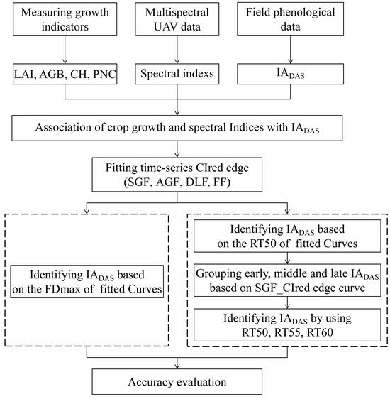
2. Materials and Methods

2.1. Study Area

In this study, selection trials of soybean varieties were conducted in two different climatic regions, Shijiazhuang City (SJZ) and Xuzhou City (XZ), from June to October 2022 (Figure 1). The SJZ site (E114°43′28″, N37°56′27″), with a total area of about 8000 m², is located in Hebei Province, with a temperate continental monsoon climate. The XZ site (E117°24′07″, N34°17′50″) with a total area of about 8000 m² is located in Jiangsu Province, with a warm–temperate semi-humid monsoon climate.

In the SJZ experiment, the soybean was sown on 1 July 2022, with 220 plots involving 55 varieties and 4 replications. The plot area was 1 m² (2 m × 0.5 m) and the row spacing was 0.5 m, respectively. In the XZ experiment, the soybean was sown on 12 June 2022. There were 110 plots with the same 55 varieties and 2 replications. The plot area was 2 m² (2 m × 1 m) and the row spacing was 0.5 m, respectively. Other field managements (pest control and herbicide application) followed the standard local practices.

2.2. Data Collection

2.2.1. UAV Data

• Flight Observation

The DJI P4 Multispectral UAV (SZ DJI Technology Co., Shenzhen, China) was used for acquiring high-throughput multispectral images during the entire growing season of soybeans in 2022. The P4M multispectral UAV carries a 2.08-Megapixel resolving power lens, integrated with six channels of visible, blue, green, red, red-edge and near-infrared. The specific parameters are shown in

Table 1. Center wavelengths and bandwidths of the P4M UAV.

Band Name	Center Wavelength (nm)	Band Width (nm)
Visible light (RGB)	-	-
Blue	450	16
Green	560	16
Red	650	16
Red edge	730	16
Near-infrared	840	26

. Prior to the mission, 12 ground control points (GCPs) were set up with black and white calibration boards for the trials at two locations, and their precise positions were measured using a GPS system. All missions were conducted between 10:00 and 14:00 on clear, cloudless and windless days. The observation frequency was once every 3–5 days, weather permitting. The UAV flight altitude was set to 20m with an 80% overlap in both heading and side directions.

The SJZ experiment was conducted from 17 July to 12 October, and the XZ experiment was conducted from 29 June to 28 September, with 17 and 21 multispectral image acquisition missions, respectively. DJI Terra software was used for image stitching and radiometric calibration, and ArcMap software version 10.2 (Environmental Systems Research Institute, Inc., Redlands, CA, USA) and ENVI software version 5.3 (Harris Geospatial Solutions, Inc., Boulder, CO, USA) were used for image-cropping, band alignment, plotting the region of interest (ROI) with the same location for each date, and extracting the average reflectance of the pixels within the ROI.

2.

Spectral Index Extraction

Vegetation indices (VIs) are commonly used to characterize the growth of vegetation and are closely related to the photosynthetic and nutrient status of the vegetation. The NDVI can reveal the greenness of vegetation and is commonly used to extract leaf area index, photosynthetic capacity, chlorophyll and biomass [37]. Green normalized-difference vegetation index (GNDVI) is often used for monitoring vegetation cover and canopy nitrogen content [38]. An enhanced vegetation index (EVI) can suppress canopy background signals and atmospheric effects, and it had good performance in leaf area index and cover monitoring [39]. Two-band enhanced vegetation index (EVI2) is commonly used to accurately assess the growth status of vegetation, including greenness, growth and drought tolerance. It can provide a more complete picture of the vegetation growth of a crop [40]. Normalized-difference red-edge index (NDRE) was sensitive to the chlorophyll content of vegetation in highly vegetated areas [41]. Red edge chlorophyll index (CIred edge) utilizes red edge reflectance and had good performance in the estimation of chlorophyll content, leaf area index and biomass [27]. These VIs play an important role in revealing the vegetation growth process and the dynamics of phenological period characteristics. In this study, these six VIs were used to identify the initial anthesis of soybean, as shown in

Table 2. Spectral vegetation indices used in this study.

Vegetation Index	Calculation Formula	Reference
Normalized-Difference Vegetation Index	NDVI = (NIR − R)/(NIR + R)	[42]
Green Normalized-Difference Vegetation Index	GNDVI = (NIR − G)/(NIR + G)	[43]
Enhanced Vegetation Index	EVI = 2.5[(NIR − R)/(NIR + 6R − 7.5B + 1)]	[44]
Two-band Enhanced Vegetation Index	EVI2 = 2.5[(NIR − R)/(NIR + 2.4R + 1)]	[45]
Normalized-Difference Red-Edge Index	NDRE = (NIR − RE)/(NIR + RE)	[46]
Red-Edge Chlorophyll Index	CIred edge = (NIR/RE) − 1	[47]

.

3.

Spectral Index Fitting Function

Noise is inevitable in the acquired multispectral image data due to the unexpected changes in weather and lighting conditions. This could affect the accuracy of phenology monitoring; thus, methods of smoothing or fitting time-series curves that can effectively de-noise and eliminate outliers are needed, e.g., symmetric gauss function (SGF) [22], asymmetric gauss function (AGF) [48], double logistic function (DLF) [23] and fourier function (FF) [26]. Each method was developed with its own merits, and it is not currently clear which one is more suitable for monitoring phenology. In order to obtain high-quality time-series VI, this study applied and compared the four fitting functions of SGF, AGF, DLF, and FF in reconstructing the phenological curves, expressed as SGF_VIs, AGF_VIs, DLF_VIs, and FF_VIs, respectively. The calculation formulas are as follows:

$$\mathrm{SGF}\_\mathrm{VI}=\mathrm{b}{\mathrm{e}}^{-{\left(\frac{\mathrm{D}\mathrm{A}\mathrm{S}-\mathrm{c}}{\mathrm{a}}\right)}^2}$$

(1)

$$\mathrm{AGF}\_\mathrm{VI}=\mathrm{d}{\mathrm{e}}^{-{\left(\frac{\mathrm{D}\mathrm{A}\mathrm{S}-\mathrm{g}}{\mathrm{f}}\right)}^2}+{\mathrm{h}\mathrm{e}}^{-{\left(\frac{\mathrm{D}\mathrm{A}\mathrm{S}-\mathrm{j}}{\mathrm{i}}\right)}^2}$$

(2)

$$\mathrm{DLF}\_\mathrm{VI}=\frac{\mathrm{k}}{\left(1+{\mathrm{e}}^{\left(\mathrm{m}+\mathrm{n}\ast \mathrm{D}\mathrm{A}\mathrm{S}\right)}\right)}+\frac{\mathrm{r}}{\left(1+{\mathrm{e}}^{\left(\mathrm{p}+\mathrm{q}\ast \mathrm{D}\mathrm{A}\mathrm{S}\right)}\right)},$$

(3)

$$\mathrm{FF}\_\mathrm{VI}=\mathrm{l}+{\sum }_{\mathrm{i}=1}^2{\mathrm{s}}_{\mathrm{i}}\times \mathrm{c}\mathrm{o}\mathrm{s}\left(\mathrm{u}\times \mathrm{v}\times \mathrm{D}\mathrm{A}\mathrm{S}\right)+{\mathrm{t}}_{\mathrm{i}}\times \mathrm{s}\mathrm{i}\mathrm{n}\left(\mathrm{u}\times \mathrm{v}\times \mathrm{D}\mathrm{A}\mathrm{S}\right)$$

(4)

where DAS is the number of days after soybean sowing, indicating that the acquisition time of VI, e is a natural constant, and a, b, c, d, f, g, h, i, j, k, l, m, n, p, q, r, s, t, u, and v are the parameters of the fitting functions, which are determined by optimization procedure in Matlab with the least square method.

2.2.2. Crop Growth Indicators

In this study, the investigated crop parameters iwere canopy height (CH), leaf area index (LAI), above-ground biomass (AGB), and plant nitrogen content (PNC). At different growth periods, eight soybean plants were randomly selected in each plot, and the height of each plant was measured with a steel ruler. The CH of the plot was determined by averaging the CH values of the eight plants. For LAI, AGB and PNC measurements, from one to three soybean plants were randomly sampled in each plot. The roots were removed, and the leaves, stalks, and pods (after the podding stage) were collected and weighed separately. The LAI was measured and calculated by the perforation method. The soybean samples were then put into paper bags, numbered and placed in the oven. The samples were first dried at 105 °C for 30 min (called blanching), and then dried at 80 °C for approximately 72 h until the weight no longer changed [49]. The dry matter of the soybean samples was weighed and recorded. The AGB per unit area was calculated from the dry matter of samples and planting density. Finally, the PNC of soybeans was measured using the Kjeldahl method [50].

2.2.3. Phenology Records and Meteorological Data

In this study, in situ field observations and records of the phenological development and IA_DAS were conducted for each plot at an interval of 2 days, following the specifications for agrometeorological observations of soybean (https://www.cma.gov.cn/zfxxgk/gknr/flfgbz/bz/202209/t20220921_5099037.html, accessed on 12 June 2022) from the China Meteorological Administration. The phenological time was recorded in terms of DAS. When the number of flowering plants in a plot was observed to be up to 10% of the total plants in that plot, the exact date was recorded as the soybean IA_DAS of this plot.

Meteorological data were obtained from the China Meteorological Data Service Center (http://data.cma.cn/, accessed on 10 January 2023), including daily maximum air temperature (Tmax), minimum air temperature (Tmin) and precipitation in both sites from June to November 2022.

2.2.4. Accuracy Evaluation Indicators

The coefficient of determination (R²), root mean square error (RMSE), and mean absolute error (MAE) were used in this study to assess the performance of the four fitted functions and the estimation accuracy of soybean IA_DAS. The mathematical models were performed using MATLAB R2018a (MathWorks, Inc., Natick, MA, USA), and graphics were produced using the Origin 2022 software program (OriginLab Inc., Northampton, MA, USA).

3. Results

3.1. Statistical Analysis of IA_DAS

In this study, the soybean IA_DAS of the two-site trial was statistically analyzed, as shown in Figure 2. The IA_DAS in the two trials ranged from DAS 26 to 50, with the mean values of DAS 34.73 and DAS 37.98, and coefficients of variation of 14.65% and 17.80% in SJZ and XZ, respectively (

Table 3. The statistical characteristics of IA_DAS.

Site	Number of Plots	Minimum	Mean	Maximum	Standard Deviation	Variance	Coefficient of Variation (%)
SJZ	220	26	34.73	47	5.09	25.88	14.65
XZ	110	26	37.98	50	6.76	45.72	17.80

). In this study, soybean varieties were divided into three groups according to their IA_DAS. The soybean materials with IA_DAS before DAS 30 were grouped into early anthesis varieties, those between DAS 31 and 40 were grouped into middle anthesis varieties, and the ones between DAS 41 and 50 were grouped into late anthesis varieties. In the two trials, there were significant differences in the IA_DAS of the different soybean varieties. In addition, the progression of soybean IA_DAS in the XZ region lagged significantly behind that in the SJZ region, reflecting the influence of different geographic environments on soybean growth processes.

3.2. Temporal Dynamics of Crop Growth and Spectral Indices Associated with Flowering Time

The temporal dynamic changes in the measured growth parameters of LAI, AGB and CH are shown in Figure 3, taking the early, middle and late soybean varieties in SJZ region as an example.

With the growth and development of soybean, the growth parameters show obvious changes at different stages. During DAS 20–60, LAI, AGB and CH showed an increasing trend in different anthesis varieties. In the range of DAS 60–80, LAI, AGB and CH showed a peak. During DAS 80–100, LAI, AGB and CH showed a decreasing trend. In the early growth stage of soybean (before DAS 30), the number of soybean leaves was relatively small, and their main functions were respiration and photosynthesis. Over time, soybean leaves gradually increased, and LAI, AGB and CH also gradually increased. When entering the anthesis stage (DAS 30–50), the root, stem and leaf of soybean experienced accelerated growth, while LAI, AGB, and CH continued to increase. Nutrients within the plant began to flow to the buds and pods, contributing to the growth processes of pollen development, pod formation and granulation. In the podding and seed-filling stage (near DAS 50–80), LAI, AGB, and CH reached their peaks, and some nutrients were translocated from plant stems and leaves to the pods and seeds of the soybean. At the maturity stage (after DAS 80), the leaves of soybean began to turn yellow and fall off, and LAI gradually declined. The CH of soybean gradually declined, the accumulation and distribution of dry matter in soybean shifted to pods and seeds, and AGB showed a decreasing trend.

Overall, the LAI, AGB and CH of early, middle and late IA_DAS varieties all showed an obvious trend of first increasing and then decreasing. This trend is consistent with the characteristics of nutrient uptake and the growth of soybean plants. The general changing trend of LAI, AGB and CH was similar in the two trials. Note that there was a decrease in the canopy height in Figure 3d,e. This was because these soybean varieties suffered lodging around DAS 45, which led to a decreased canopy height.

The canopy multispectral images of the soybean varieties with early, middle and late IA_DAS are shown in Figure 4a, and the canopy reflectance of the five bands at different growth stages are shown in Figure 4b–d. Overall, with the development of the soybean growth, the reflectance of the five spectral bands showed a trend of first increasing and then decreasing, especially in the red-edge and near-infrared bands. With the delayed IA_DAS of soybean varieties, the spectral reflectance was significantly different among the soybean canopies with early, middle and late IA_DAS, and there was a significant gradual increase in the reflectance of the red-edge and near-infrared bands.

The time-series dynamic changes in the NDVI, GNDVI, EVI, EVI2, and NDRE are shown in Figure 5, in which the early, middle and late anthesis varieties of SJZ are presented as an example and the green dotted lines indicate the IA_DAS of each variety, respectively. It can be seen that these vegetation indices changed similarly, with an initial increase followed by a decrease, aligning with the typical growth dynamics of vegetation. After soybean emergence, NDVI, GNDVI, EVI, EVI2, and NDRE rapidly increased, and reached their maximum around DAS 40. Subsequently, NDVI and GNDVI remained stable between DAS 40 and 80, with values close to 0.9 and 0.8, respectively. EVI and EVI2 also stayed near 0.9 from DAS 35–75, while NDRE remained at approximately 0.3 from DAS 50–75. When this entered the maturity stage around DAS 80, all five indices showed a rapid decline. For a wide variety of soybean materials, like early, middle, and late flowering varieties, the spectral curves of these five indices became saturated at different time positions, like before, after, and near anthesis (near DAS 40), making it difficult to extract consistent features from them to monitor the soybean IA_DAS.

The temporal changes in the CIred edge of the early-, middle-, and late-anthesis varieties in both SJZ and XZ sites are shown in Figure 6. The overall changing trend of the CIred edge seemed similar to that of the above-mentioned five Vis; that is, first an increase in the peak values and then a decrease in the growth period. However, it was noticed an inflection point was noticed in the CIred edge spectral curve near the anthesis for all the soybean varieties, regardless of early, middle, and late flowering, suggesting that this kind of inflection point (like the FDmax) in the CIred edge time-series curve could be useful to identify soybean IA_DAS. Furthermore, with the delay in IA_DAS, the CIred edge curves of different anthesis varieties gradually increased. As shown in Figure 6, at the time of IA_DAS, the CIred edge values of early-, middle-, and late-anthesis varieties in the SJZ region were approximately 52%, 58% and 60% of the peak value of the curves, respectively. In the XZ region, the CIred edge values at the date of IA_DAS for the early-, middle-, and late-anthesis varieties were approximately 54%, 53% and 58% of the peak value of the curves. Overall, when soybean varieties were at IA_DAS, the CIred edge values were about 50–60% of the peak in the curves, with an increasing percentage of the delaying IA_DAS. These findings made it possible to use the relative threshold method to identify IA_DAS.

In addition, the peak values of the CIred edge in the SJZ trial were generally found to be greater than those in the XZ trial (Figure 6). As the CIred edge has been shown to be an accurate measure of chlorophyll [51,52] and there is a high positive correlation between chlorophyll content and nitrogen content [53], the plant nitrogen content (PNC) measured in the two trial sites is shown in Figure 7 to clarify this point. The results showed that the PNC of soybean in the XZ site was higher than that in the SJZ site from Days 50 to 80, which may be the factor that results in the higher CIred edge peak in the XZ site. Furthermore, some noise appeared in the time-series of the CIred edge, as shown in Figure 6e,f. This is inevitable in the field data collection; hence, smoothing and fitting methods are needed to reconstruct the time-series curves of VIs, as mentioned earlier.

3.3. Identifying IA_DAS with FDmax of CIred Edge-Fitting Curves

3.3.1. Fitting the CIred Edge Curve

In this study, four fitting functions, SGF, AGF, DLF, and FF, were used to fit the CIred edge spectral indices. Figure 8 demonstrates the original points of the CIred edge and its fitted phenology curves. The results showed that the SGF function provided a better fitting in the early stage of soybean (before DAS 50), and it can effectively eliminate the noise and outliers. The AGF function performed well in fitting at the soybean maturity stage (DAS 70–110), but it was too sensitive to the original points, and thus was easily affected by the outliers. The DLF and FF functions provided a better performance in fitting the peak periods of the CIred edge (DAS 50–70), but the FF tended to suffer from overfitting near the start and end points.

Table 4. Performance of model fitting CIred edge.

Site	Number of Plots	Fitting Functions	R2			RMSE
			Minimum	Mean	Maximum	Minimum	Mean	Maximum
SJZ	220	SGF	0.885	0.949	0.997	0.012	0.050	0.084
		AGF	0.920	0.972	0.998	0.013	0.042	0.071
		DLF	0.905	0.971	0.998	0.011	0.033	0.058
		FF	0.921	0.973	0.998	0.014	0.041	0.073
XZ	110	SGF	0.812	0.921	0.982	0.030	0.091	0.182
		AGF	0.823	0.967	0.994	0.029	0.061	0.122
		DLF	0.842	0.969	0.996	0.021	0.047	0.099
		FF	0.867	0.969	0.994	0.033	0.059	0.112

summarizes the four functions’ fitting performances for the time-series CIred edge in terms of R² and RMSE. The R² and RMSE values for the SGF fitting ranged from 0.88 to 0.99 and from 0.012 to 0.182, respectively. The fitting R² and RMSE from the AGF, DLF, and FF were 0.82–0.99 and 0.013–0.122, 0.84–0.99 and 0.011–0.099, and 0.86–0.99 and 0.014–0.112, respectively. It was shown that the fitted CIred edge curves from the four functions (i.e., AGF_CIred edge, SGF_CIred edge, DLF_CIred edge and FF_CIred edge) all had good correlations with the original CIred edge points, and can reduce the noises and reconstruct the temporal development curves of the CIred edge.

Overall, it is hard to say which function’s fitted result is more suitable for the IA_DAS identification of soybean at present; thus all of them are further examined in the following IA_DAS identification.

3.3.2. Identification of IA_DAS Based on the FDmax of the Fitted CIred Edge Curves

The FDmax was extracted from the SGF_CIred edge, the AGF_CIred edge, the DLF_CIred edge, and the FF_CIred edge curves to identify the soybean IA_DAS. Figure 9 shows the relationships between the actual observation IA_DAS and the estimated IA_DAS from this method. For the SJZ trial, the R² of the linear relationships between the measured IA_DAS and the estimated IA_DAS with the FDmax from the SGF_CIred edge, AGF_CIred edge, DLF_CIred edge, and FF_CIred edge curves were 0.46, 0.038, 0.024, and 0.021, respectively, with an RMSE of 3.81, 7.15, 6.15, and 6.19 days and an MAE of 3.17, 6.09, 5.30, and 5.09 days, respectively. For the XZ trial, the R² of the results from the SGF_CIred edge, AGF_CIred edge, DLF_CIred edge, and FF_CIred edge curves were 0.70, 0.39, 0.53, and 0.47, respectively; the corresponding RMSEs were 3.78, 12.95, 9.98 and 11.47 days, and the MAEs were 3.00, 10.68, 8.19 and 9.37 days, respectively.

It was shown that the FDmax from SGF_CIred edge curves provided the highest identification accuracy for both SJZ and XZ trials, with an R² of 0.46 and 0.70, RMSE of 3.81 and 3.78 days, and MAE of 3.17 and 3.00 days, respectively. In contrast, the identification accuracy from the FDmax of the DLF_CIred edge and FF_CIred edge curves was relatively lower than that of the SGF_CIred edge curve. The RMSE values from the DLF_CIred edge and FF_CIred edge curves were 6.15 and 6.19 days for the SJZ trial, and 9.98 and 11.47 days for the XZ trial, respectively. The identification accuracy from the FDmax of AGF_CIred edge curve was found to be much lower than that of the other three, with an RMSE of 7.15 and 12.95 days for the SJZ and XZ trials, respectively. Therefore, the FDmax of the SGF_CIred edge curve was considered to be an effective feature for identifying the soybean IA_DAS.

3.4. Identifying the IA_DAS Based on Relative Thresholds of Fitted CIred Edge Curves

3.4.1. Identifying Soybean IA_DAS Based on a Single Relative Threshold for All Varieties

The relative threshold method was also examined in this study to identify soybean IA_DAS. Based on the results stated earlier, 50% of the maximum value (RT50) of the CIred edge curve was used as a single relative threshold for identifying the IA_DAS of all the soybean varieties. The results with the RT50 from the SGF_CIred edge, AGF_CIred edge, DLF_CIred edge, and FF_CIred edge curves are shown in Figure 10.

It was shown that the RT50 of the SGF_CIred edge phenology curve demonstrated the best recognition accuracy in both SJZ and XZ sites, with an R² of 0.451 and 0.683, RMSE of 4.85 and 4.37 days, and MAE values of 3.81 and 3.71 days, respectively. The accuracy of the IA_DAS estimated using the RT50 from the DLF_CIred edge and FF_CIred edge curves was comparable: in the SJZ site, the results from the FF_CIred edge curve (RMSE = 5.16 days, MAE = 4.12 days) were slightly better than those of the DLF_Cired edge curve (RMSE = 5.81 days, MAE = 4.76 days), while, in the XZ site, the accuracy from the DLF_CIred edge curve (RMSE = 5.76 days, MAE = 4.49 days) was slightly higher than that of the FF_CIred edge curve (RMSE = 6.45 days, MAE = 5.07 days). The identification accuracy of IA_DAS with the RT50 from the AGF_CIred edge was lower compared with that of the above-mentioned three curves, with an R² of 0.041 and 0.369, RMSE greater than 6 days, and MAE greater than 5 days for the SJZ and XZ sites.

Furthermore, the relationships between the measured IA_DAS and the estimated IA_DAS with the RT50 of the SGF_CIred edge curves for both sites are presented in Figure 11. It was found that the IA_DAS of the delayed anthesis varieties was generally underestimated; for example, the middle-anthesis varieties with IA_DAS between DAS 35 and 40 and the late-anthesis varieties with IA_DAS between DAS 40 and 50. This may be associated with the delayed-anthesis varieties having greater percentages of the CIred edge value from flowering to maximum, as mentioned earlier. Therefore, it would be beneficial to use different relative thresholds for the early, middle and late anthesis to improve the IA_DAS identification.

3.4.2. Identifying IA_DAS by Using Different Relative Thresholds for Early, Middle and Late Anthesis Varieties

Based on the above analysis, the identification of soybean IA_DAS was further established using the relative threshold method combined with the variety groups of early, middle, and late anthesis.

The SGF_CIred edge curve, which showed the best performance in IA_DAS identification according to the above results, was used here to group the soybean varieties into early, middle, and late anthesis categories. It was found that the area under the SGF_CIred edge curve, from the starting point to the peak, can be used as an effective indicator to divide the varieties into early, middle and late anthesis groups, as shown in Figure 12. Additionally, the area values, which were normalized and sorted in ascending order, are presented in Figure 13. It was shown that the distribution of the area points was uniform and continuous between the locations of 42 and 185 for the SJZ trial, and between locations 22 and 77 for the XZ trial. Therefore, for the SJZ and XZ trials, the top 42 and 22 in the area rankings were grouped as early-anthesis varieties, 43–185 and 78–110 were grouped as middle-anthesis varieties, and 186–220 and 78–110 were grouped as the late-anthesis varieties, respectively.

According to the results, the CIred edge values at IA_DAS were about 50–60% of the peak of the curves, and the percentage tended to increase with the delay in IA_DAS. Therefore, the 50%, 55%, and 60% of the peak values of the SGF_CIred edge curves, expressed as RT50, RT55 and RT60, were used as three respective thresholds for the early-, middle-, and late-anthesis varieties to improve the identification of IA_DAS. The estimated results are presented in Figure 14, with an improved accuracy compared with the identification obtained by using a single threshold (RT50). Specifically, for the SJZ trial, the RMSE decreased from 4.84 days to 3.69 days, and the MAE decreased from 3.84 days to 3.09 days. For the XZ trial, the RMSE decreased from 4.37 days to 3.81 days and the MAE decreased from 3.71 days to 3.19 days. The R² for both trials also increased to different degrees. In particular, the estimations of IA_DAS for both the middle and late anthesis varieties were significantly improved using the respective relative thresholds of RT55 and RT60 instead of the single-threshold RT50, with an estimated IA_DAS that was much closer to the observed ones. Therefore, when using the relative threshold method to identify soybean IA_DAS, it is suggested to use different thresholds for different anthesis varieties.

4. Discussion

4.1. Merits of CIred Edge Temporal Curves in Soybean IA_DAS Identification

The time-series of NDVI, GNDVI, EVI, EVI2 and NDRE were found to be useful in monitoring vegetation phenology [41,54,55,56,57]. However, the time-series curves of these vegetation indices tend toward saturation when soybean plants have dense foliage, making it difficult to extract useful features for the accurate identification of the IA_DAS. By contrast, the CIred edge curves showed no saturation throughout the soybean season, making them more suitable for identifying the IA_DAS. In addition, with the growth and development of soybean, the reflectance in the red-edge band and near-infrared band had an obvious trend of first increasing and then decreasing, especially among the early, middle, and late soybean varieties with distinct IA_DAS. It was demonstrated that the CIred edge time series performed well and consistently in soybean IA_DAS identification at two different experimental sites, with an RMSE of 3.69–3.81 days and MAE of 3.0–3.2 days, respectively.

4.2. Comparison of Methods for IA_DAS Identification

The IA_DAS identification in this study was mainly based on the CIred edge time-series curves, the methods of change detection (like the FDmax) and the relative threshold. The choice of the fitting function for VI time-series data would have an effect on the identification accuracy of IA_DAS. In reconstructing the time-series CIred edge phenology curves, this study used four fitting functions of SGF, AGF, DLF and FF. There are 3, 6, 6 and 6 parameters, respectively, in the SGF, AGF, DLF and FF models. It is known that the function that has more parameters generally provides a better fitting; at the same time, it has a higher risk of overfitting (R² = 1, RMSE = 0). At both trial sites in this study, the Cired edge curves fitted by the SGF had a slightly lower R² and bigger RMSE compared with those fitted by AGF, DLF and FF. However, the identification accuracy of soybean IA_DAS from the SGF-fitted CIred edge curves was much higher (RMSE and MAE = 3.0–5.0 days) than that from the curves fitted by AGF, DLF and FF (RMSE and MAE = 5.0–12.0 days). This was probably due to the overfitting of the CIred edge time-series curves by AGF, DLF, and FF, which would suppress the important phenological features and lead to a larger estimation error. Furthermore, the SGF could effectively filter the noises and outliers [28] and reconstruct the CIred edge curves more accurately, which may contribute to its better performance in identifying IA_DAS.

As for the characteristic parameters used to identify the IA_DAS, the FDmax was adopted first as a key feature point to identify the position of IA_DAS in the phonological curves. The FDmax from the SGF-fitted CIred edge curves (as mentioned above) led to the best accuracy in IA_DAS identification, with RMSE = 3.81 days, MAE = 3.17 days for the SJZ site and RMSE = 3.79 days, MAE = 3.00 days for the XZ, respectively. There are some reasons for this. Flowering indicates the beginning of the reproductive and nutrient growth of crops, and this process will have a significant impact on crop nutrient partitioning [58]. Once soybean is flowering, the flow rate from nutrients to canopy leaves slows down, which would result in a decrease in the rate of canopy development and a corresponding change in the spectral response of the soybean canopy. Thus, the FDmax, which means the maximum growth rate that the canopy reaches, can reflect the initial anthesis, i.e., IA_DAS.

In addition to the FDmax, the relative thresholds of the time-series CIred edge curves were also tried in this study as feature points for IA_DAS identification. At first, a single relative threshold of RT50 was adopted for all soybean varieties to identify IA_DAS. The best accuracy was obtained from the SGF-fitted CIred edge curves (as mentioned above). The RMSE = 4.85 days, MAE = 3.81 days for SJZ site and the RMSE = 4.37 days, MAE = 3.71 days for XZ site, respectively, which were relatively larger than that of the FDmax method. In particular, bigger errors were observed in the soybean varieties with a relatively late anthesis compared with the others (Figure 12). In view of this, the soybean varieties were divided into three groups of early-, middle-, and late-anthesis using the SGF_CIred edge curves, and adopted three different relative thresholds (e.g., RT50, RT55, RT60) for each group (e.g., early, middle, and late), respectively. The method can reduce the identification errors in the middle- and late-anthesis soybean varieties, and thus improve the IA_DAS accuracy, with an RMSE = 3.69 days, MAE = 3.09 days for SJZ site and RMSE = 3.81 days, MAE = 3.19 days for the XZ site, respectively. This was very similar to that of the FDmax method. Therefore, it was proposed that the FDmax method, and the relative threshold method, combined with a grouping of the soybean varieties into early-, middle-, and late-anthesis, can be used to effectively identify the soybean IA_DAS.

4.3. Variations of Soybean IA_DAS under Different Climatic Conditions

There are many factors affecting crop phenology, such as variety, light, temperature, and fertilizer application [59]. In this study, soybean varieties, temperature, and precipitation were investigated. Variety has a direct effect on the growth and development process of soybean, and thus is the primary factor influencing the anthesis of soybean. The IA_DAS of different soybean varieties in the same region varied considerably. The earliest IA_DAS among the soybean varieties in both regions of XZ and SJZ appeared on DAS 26, and the latest were DAS 47 and DAS 50, respectively. In addition, the IA_DAS of the same varieties also differed between the XZ and SJZ regions (Figure 15). The mean IA_DAS in SJZ and XZ regions were DAS 34.73 and DAS 37.98, respectively, and it was relatively delayed in the XZ region. This may be because soybean is a kind of crop that is very sensitive to weather factors like high temperature and rains, and continuous high-temperature or rainy days would significantly affect the growth process of soybean, and cause a delay in the phenology. Figure 16 shows that the temperature was relatively higher during the period of DAS 20–50 in the XZ region than that in the SJZ, accompanied by higher daily precipitation and more continuous rainy days. This may explain the relatively delayed anthesis in the XZ region.

In addition, it was shown in Figure 16 that constant hot weather (Tmax ≥ 35 °C) occurred in DAS 50–70 in the XZ region, and there was also a dramatic change in the temperature in DAS 70–80. High temperature and intense sunlight can cause changes in leaf structure and result in exceptions to the spectral response in the NIR band. This may account for the abnormal fluctuations in VIs between DAS 60 and 80 in the XZ region (Figure 6f). Therefore, it is necessary to adopt smoothing and fitting methods to eliminate noise and outliers when applying the time-series CIred edge to recognize soybean’s initial anthesis.

5. Conclusions

The main goal of this study was to explore a high-throughput remote method for identifying the initial day of anthesis of soybean varieties in field trials based on multispectral time-series images collected by UAV during the growth season. It was found that the phenological development of soybean varieties can be reflected by the time series of the CIred edge without saturation compared with the NDVI and other indices, and thus the CIred edge was chosen to identify soybean IA_DAS in this study. Based on the CIred edge time-series curves fitted with the SGF function, the FDmax feature was extracted and provided effective estimates of the IA_DAS with an RMSE and MAE of 3.79 days and 3.00 days, respectively. The relative threshold of the CIred edge time-series curves was also effective for extracting soybean IA_DAS, especially by combining the flowering time characteristics of soybean varieties, that is, using different relative thresholds (e.g., RT50, RT55, RT60) for different flowering groups (e.g., early, middle, and late). The RMSE and MAE were 3.69 days and 3.09 days, respectively. Thus, the two methods can be used as efficient tools to accurately identify the initial anthesis (IA_DAS) of soybean varieties by UAV multispectral remote sensing, and are expected to be beneficial for promoting crop germplasm resources and breeding selection. In addition, it was shown that the soybean IA_DAS, even for the same varieties, differed significantly in two different regions with distinct climatic conditions due to the genotype–environment interactions, indicating the importance of conducting various field trials in different regions to identify the superior cultivars in crop breeding studies.

References

1. Lee, C.; Choi, M.-S.; Kim, H.-T.; Yun, H.-T.; Lee, B.; Chung, Y.-S.; Kim, R.W.; Choi, H.-K. Soybean [Glycine max (L.) Merrill]: Importance as a crop and pedigree reconstruction of Korean varieties. Plant Breed. Biotechnol. 2015, 3, 179–196. [Google Scholar] [CrossRef]
2. Moeinizade, S.; Pham, H.; Han, Y.; Dobbels, A.; Hu, G. An applied deep learning approach for estimating soybean relative maturity from UAV imagery to aid plant breeding decisions. Mach. Learn. Appl. 2022, 7, 100233. [Google Scholar] [CrossRef]
3. Liu, S.; Zhang, M.; Feng, F.; Tian, Z. Toward a “green revolution” for soybean. Mol. Plant 2020, 13, 688–697. [Google Scholar] [CrossRef] [PubMed]
4. Araus, J.L.; Cairns, J.E. Field high-throughput phenotyping: The new crop breeding frontier. Trends Plant Sci. 2014, 19, 52–61. [Google Scholar] [CrossRef] [PubMed]
5. Jin, X.; Zarco-Tejada, P.J.; Schmidhalter, U.; Reynolds, M.P.; Hawkesford, M.J.; Varshney, R.K.; Yang, T.; Nie, C.; Li, Z.; Ming, B. High-throughput estimation of crop traits: A review of ground and aerial phenotyping platforms. IEEE Geosci. Remote Sens. Mag. 2020, 9, 200–231. [Google Scholar] [CrossRef]
6. Furbank, R.T.; Jimenez-Berni, J.A.; George-Jaeggli, B.; Potgieter, A.B.; Deery, D.M. Field crop phenomics: Enabling breeding for radiation use efficiency and biomass in cereal crops. New Phytol. 2019, 223, 1714–1727. [Google Scholar] [CrossRef]
7. Jangra, S.; Chaudhary, V.; Yadav, R.C.; Yadav, N.R. High-throughput phenotyping: A platform to accelerate crop improvement. Phenomics 2021, 1, 31–53. [Google Scholar]
8. Duan, B.; Fang, S.; Gong, Y.; Peng, Y.; Wu, X.; Zhu, R. Remote estimation of grain yield based on UAV data in different rice cultivars under contrasting climatic zone. Field Crops Res. 2021, 267, 108148. [Google Scholar] [CrossRef]
9. Xie, C.; Yang, C. A review on plant high-throughput phenotyping traits using UAV-based sensors. Comput. Electron. Agric. 2020, 178, 105731. [Google Scholar] [CrossRef]
10. Feng, L.; Chen, S.; Zhang, C.; Zhang, Y.; He, Y. A comprehensive review on recent applications of unmanned aerial vehicle remote sensing with various sensors for high-throughput plant phenotyping. Comput. Electron. Agric. 2021, 182, 106033. [Google Scholar]
11. Tayade, R.; Yoon, J.; Lay, L.; Khan, A.L.; Yoon, Y.; Kim, Y. Utilization of spectral indices for high-throughput phenotyping. Plants 2022, 11, 1712. [Google Scholar] [CrossRef] [PubMed]
12. Roosjen, P.P.; Brede, B.; Suomalainen, J.M.; Bartholomeus, H.M.; Kooistra, L.; Clevers, J.G. Improved estimation of leaf area index and leaf chlorophyll content of a potato crop using multi-angle spectral data–potential of unmanned aerial vehicle imagery. Int. J. Appl. Earth Obs. Geoinf. 2018, 66, 14–26. [Google Scholar] [CrossRef]
13. Yue, J.; Yang, G.; Tian, Q.; Feng, H.; Xu, K.; Zhou, C. Estimate of winter-wheat above-ground biomass based on UAV ultrahigh-ground-resolution image textures and vegetation indices. ISPRS J. Photogramm. Remote Sens. 2019, 150, 226–244. [Google Scholar]
14. Qiao, L.; Tang, W.; Gao, D.; Zhao, R.; An, L.; Li, M.; Sun, H.; Song, D. UAV-based chlorophyll content estimation by evaluating vegetation index responses under different crop coverages. Comput. Electron. Agric. 2022, 196, 106775. [Google Scholar] [CrossRef]
15. Han, L.; Yang, G.; Yang, H.; Xu, B.; Li, Z.; Yang, X. Clustering field-based maize phenotyping of plant-height growth and canopy spectral dynamics using a UAV remote-sensing approach. Front. Plant Sci. 2018, 9, 1638. [Google Scholar] [CrossRef]
16. Guo, Y.; Xiao, Y.; Li, M.; Hao, F.; Zhang, X.; Sun, H.; de Beurs, K.; Fu, Y.H.; He, Y. Identifying crop phenology using maize height constructed from multi-sources images. Int. J. Appl. Earth Obs. Geoinf. 2022, 115, 103121. [Google Scholar] [CrossRef]
17. Lyu, M.; Lu, X.; Shen, Y.; Tan, Y.; Wan, L.; Shu, Q.; He, Y.; He, Y.; Cen, H. UAV time-series imagery with novel machine learning to estimate heading dates of rice accessions for breeding. Agric. For. Meteorol. 2023, 341, 109646. [Google Scholar] [CrossRef]
18. Vrieling, A.; Skidmore, A.K.; Wang, T.; Meroni, M.; Ens, B.J.; Oosterbeek, K.; O’Connor, B.; Darvishzadeh, R.; Heurich, M.; Shepherd, A. Spatially detailed retrievals of spring phenology from single-season high-resolution image time series. Int. J. Appl. Earth Obs. Geoinf. 2017, 59, 19–30. [Google Scholar] [CrossRef]
19. Zhang, X.; Goldberg, M.D. Monitoring fall foliage coloration dynamics using time-series satellite data. Remote Sens. Environ. 2011, 115, 382–391. [Google Scholar] [CrossRef]
20. Gan, L.; Cao, X.; Chen, X.; Dong, Q.; Cui, X.; Chen, J. Comparison of MODIS-based vegetation indices and methods for winter wheat green-up date detection in Huanghuai region of China. Agric. For. Meteorol. 2020, 288, 108019. [Google Scholar] [CrossRef]
21. Zhao, F.; Yang, G.; Yang, X.; Cen, H.; Zhu, Y.; Han, S.; Yang, H.; He, Y.; Zhao, C. Determination of key phenological phases of winter wheat based on the time-weighted dynamic time warping algorithm and MODIS time-series data. Remote Sens. 2021, 13, 1836. [Google Scholar] [CrossRef]
22. Jonsson, P.; Eklundh, L. Seasonality extraction by function fitting to time-series of satellite sensor data. IEEE Trans. Geosci. Remote Sens. 2002, 40, 1824–1832. [Google Scholar] [CrossRef]
23. Zhang, X.; Friedl, M.A.; Schaaf, C.B.; Strahler, A.H.; Hodges, J.C.; Gao, F.; Reed, B.C.; Huete, A. Monitoring vegetation phenology using MODIS. Remote Sens. Environ. 2003, 84, 471–475. [Google Scholar] [CrossRef]
24. Cao, R.; Chen, Y.; Shen, M.; Chen, J.; Zhou, J.; Wang, C.; Yang, W. A simple method to improve the quality of NDVI time-series data by integrating spatiotemporal information with the Savitzky-Golay filter. Remote Sens. Environ. 2018, 217, 244–257. [Google Scholar] [CrossRef]
25. Sakamoto, T.; Yokozawa, M.; Toritani, H.; Shibayama, M.; Ishitsuka, N.; Ohno, H. A crop phenology detection method using time-series MODIS data. Remote Sens. Environ. 2005, 96, 366–374. [Google Scholar] [CrossRef]
26. Olsson, L.; Eklundh, L. Fourier series for analysis of temporal sequences of satellite sensor imagery. Int. J. Remote Sens. 1994, 15, 3735–3741. [Google Scholar] [CrossRef]
27. Zheng, H.; Cheng, T.; Yao, X.; Deng, X.; Tian, Y.; Cao, W.; Zhu, Y. Detection of rice phenology through time series analysis of ground-based spectral index data. Field Crops Res. 2016, 198, 131–139. [Google Scholar] [CrossRef]
28. Ma, Y.; Jiang, Q.; Wu, X.; Zhu, R.; Gong, Y.; Peng, Y.; Duan, B.; Fang, S. Monitoring hybrid rice phenology at initial heading stage based on low-altitude remote sensing data. Remote Sens. 2020, 13, 86. [Google Scholar] [CrossRef]
29. Guo, Y.; Fu, Y.H.; Chen, S.; Bryant, C.R.; Li, X.; Senthilnath, J.; Sun, H.; Wang, S.; Wu, Z.; de Beurs, K. Integrating spectral and textural information for identifying the tasseling date of summer maize using UAV based RGB images. Int. J. Appl. Earth Obs. Geoinf. 2021, 102, 102435. [Google Scholar] [CrossRef]
30. Zeng, L.; Wardlow, B.D.; Xiang, D.; Hu, S.; Li, D. A review of vegetation phenological metrics extraction using time-series, multispectral satellite data. Remote Sens. Environ. 2020, 237, 111511. [Google Scholar]
31. Sakamoto, T.; Wardlow, B.D.; Gitelson, A.A.; Verma, S.B.; Suyker, A.E.; Arkebauer, T.J. A two-step filtering approach for detecting maize and soybean phenology with time-series MODIS data. Remote Sens. Environ. 2010, 114, 2146–2159. [Google Scholar] [CrossRef]
32. Yang, Q.; Shi, L.; Han, J.; Yu, J.; Huang, K. A near real-time deep learning approach for detecting rice phenology based on UAV images. Agric. For. Meteorol. 2020, 287, 107938. [Google Scholar] [CrossRef]
33. Liu, L.; Cao, R.; Chen, J.; Shen, M.; Wang, S.; Zhou, J.; He, B. Detecting crop phenology from vegetation index time-series data by improved shape model fitting in each phenological stage. Remote Sens. Environ. 2022, 277, 113060. [Google Scholar] [CrossRef]
34. Zhou, M.; Ma, X.; Wang, K.; Cheng, T.; Tian, Y.; Wang, J.; Zhu, Y.; Hu, Y.; Niu, Q.; Gui, L. Detection of phenology using an improved shape model on time-series vegetation index in wheat. Comput. Electron. Agric. 2020, 173, 105398. [Google Scholar] [CrossRef]
35. Yu, N.; Li, L.; Schmitz, N.; Tian, L.F.; Greenberg, J.A.; Diers, B.W. Development of methods to improve soybean yield estimation and predict plant maturity with an unmanned aerial vehicle based platform. Remote Sens. Environ. 2016, 187, 91–101. [Google Scholar] [CrossRef]
36. Zhang, S.; Feng, H.; Han, S.; Shi, Z.; Xu, H.; Liu, Y.; Feng, H.; Zhou, C.; Yue, J. Monitoring of Soybean Maturity Using UAV Remote Sensing and Deep Learning. Agriculture 2022, 13, 110. [Google Scholar] [CrossRef]
37. Zeng, Y.; Hao, D.; Huete, A.; Dechant, B.; Berry, J.; Chen, J.M.; Joiner, J.; Frankenberg, C.; Bond-Lamberty, B.; Ryu, Y. Optical vegetation indices for monitoring terrestrial ecosystems globally. Nat. Rev. Earth Environ. 2022, 3, 477–493. [Google Scholar] [CrossRef]
38. Padilla, F.M.; Peña-Fleitas, M.T.; Gallardo, M.; Thompson, R.B. Evaluation of optical sensor measurements of canopy reflectance and of leaf flavonols and chlorophyll contents to assess crop nitrogen status of muskmelon. Eur. J. Agron. 2014, 58, 39–52. [Google Scholar] [CrossRef]
39. Vijith, H.; Dodge-Wan, D. Applicability of MODIS land cover and Enhanced Vegetation Index (EVI) for the assessment of spatial and temporal changes in strength of vegetation in tropical rainforest region of Borneo. Remote Sens. Appl. Soc. Environ. 2020, 18, 100311. [Google Scholar] [CrossRef]
40. Tian, F.; Cai, Z.; Jin, H.; Hufkens, K.; Scheifinger, H.; Tagesson, T.; Smets, B.; Van Hoolst, R.; Bonte, K.; Ivits, E. Calibrating vegetation phenology from Sentinel-2 using eddy covariance, PhenoCam, and PEP725 networks across Europe. Remote Sens. Environ. 2021, 260, 112456. [Google Scholar] [CrossRef]
41. Jorge, J.; Vallbé, M.; Soler, J.A. Detection of irrigation inhomogeneities in an olive grove using the NDRE vegetation index obtained from UAV images. Eur. J. Remote Sens. 2019, 52, 169–177. [Google Scholar] [CrossRef]
42. Tucker, C.J. Red and photographic infrared linear combinations for monitoring vegetation. Remote Sens. Environ. 1979, 8, 127–150. [Google Scholar] [CrossRef]
43. Gitelson, A.A.; Kaufman, Y.J.; Merzlyak, M.N. Use of a green channel in remote sensing of global vegetation from EOS-MODIS. Remote Sens. Environ. 1996, 58, 289–298. [Google Scholar] [CrossRef]
44. Huete, A.; Didan, K.; Miura, T.; Rodriguez, E.P.; Gao, X.; Ferreira, L.G. Overview of the radiometric and biophysical performance of the MODIS vegetation indices. Remote Sens. Environ. 2002, 83, 195–213. [Google Scholar] [CrossRef]
45. Jiang, Z.; Huete, A.R.; Didan, K.; Miura, T. Development of a two-band enhanced vegetation index without a blue band. Remote Sens. Environ. 2008, 112, 3833–3845. [Google Scholar] [CrossRef]
46. Daughtry, C.S.; Walthall, C.; Kim, M.; De Colstoun, E.B.; McMurtrey Iii, J. Estimating corn leaf chlorophyll concentration from leaf and canopy reflectance. Remote Sens. Environ. 2000, 74, 229–239. [Google Scholar] [CrossRef]
47. Gitelson, A.A.; Gritz, Y.; Merzlyak, M.N. Relationships between leaf chlorophyll content and spectral reflectance and algorithms for non-destructive chlorophyll assessment in higher plant leaves. J. Plant Physiol. 2003, 160, 271–282. [Google Scholar] [CrossRef]
48. Kandasamy, S.; Baret, F.; Verger, A.; Neveux, P.; Weiss, M. A comparison of methods for smoothing and gap filling time series of remote sensing observations–application to MODIS LAI products. Biogeosciences 2013, 10, 4055–4071. [Google Scholar] [CrossRef]
49. Xu, S.; Xu, X.; Zhu, Q.; Meng, Y.; Yang, G.; Feng, H.; Yang, M.; Zhu, Q.; Xue, H.; Wang, B. Monitoring leaf nitrogen content in rice based on information fusion of multi-sensor imagery from UAV. Precis. Agric. 2023, 24, 2327–2349. [Google Scholar] [CrossRef]
50. Xu, S.; Xu, X.; Blacker, C.; Gaulton, R.; Zhu, Q.; Yang, M.; Yang, G.; Zhang, J.; Yang, Y.; Yang, M. Estimation of Leaf Nitrogen Content in Rice Using Vegetation Indices and Feature Variable Optimization with Information Fusion of Multiple-Sensor Images from UAV. Remote Sens. 2023, 15, 854. [Google Scholar] [CrossRef]
51. Gitelson, A.A.; Viña, A.; Ciganda, V.; Rundquist, D.C.; Arkebauer, T.J. Remote estimation of canopy chlorophyll content in crops. Geophys. Res. Lett. 2005, 32, L08403. [Google Scholar] [CrossRef]
52. Ciganda, V.; Gitelson, A.; Schepers, J. Non-destructive determination of maize leaf and canopy chlorophyll content. J. Plant Physiol. 2009, 166, 157–167. [Google Scholar] [CrossRef] [PubMed]
53. Li, D.; Chen, J.M.; Yan, Y.; Zheng, H.; Yao, X.; Zhu, Y.; Cao, W.; Cheng, T. Estimating leaf nitrogen content by coupling a nitrogen allocation model with canopy reflectance. Remote Sens. Environ. 2022, 283, 113314. [Google Scholar] [CrossRef]
54. Zhang, C.; Xie, Z.a.; Shang, J.; Liu, J.; Dong, T.; Tang, M.; Feng, S.; Cai, H. Detecting winter canola (Brassica napus) phenological stages using an improved shape-model method based on time-series UAV spectral data. Crop J. 2022, 10, 1353–1362. [Google Scholar] [CrossRef]
55. Nguy-Robertson, A.; Gitelson, A.; Peng, Y.; Walter-Shea, E.; Leavitt, B.; Arkebauer, T. Continuous monitoring of crop reflectance, vegetation fraction, and identification of developmental stages using a four band radiometer. Agron. J. 2013, 105, 1769–1779. [Google Scholar] [CrossRef]
56. Kleinsmann, J.; Verbesselt, J.; Kooistra, L. Monitoring Individual Tree Phenology in a Multi-Species Forest Using High Resolution UAV Images. Remote Sens. 2023, 15, 3599. [Google Scholar] [CrossRef]
57. Pastor-Guzman, J.; Dash, J.; Atkinson, P.M. Remote sensing of mangrove forest phenology and its environmental drivers. Remote Sens. Environ. 2018, 205, 71–84. [Google Scholar] [CrossRef]
58. Wang, S.; Wu, Z.; Gong, Y.; Wang, S.; Zhang, W.; Zhang, S.; De Boeck, H.J.; Fu, Y.H. Climate warming shifts the time interval between flowering and leaf unfolding depending on the warming period. Sci. China Life Sci. 2022, 65, 2316–2324. [Google Scholar] [CrossRef]
59. Araya, S.; Ostendorf, B.; Lyle, G.; Lewis, M. CropPhenology: An R package for extracting crop phenology from time series remotely sensed vegetation index imagery. Ecol. Inform. 2018, 46, 45–56. [Google Scholar] [CrossRef]
Figure 1. Location of the experimental sites.
Remotesensing 15 05413 g001
Figure 2. The statistics of IADAS: (a) SJZ; (b) XZ.
Remotesensing 15 05413 g002
Figure 3. Variation in crop growth indicators in SJZ: (a) early-anthesis varieties LAI and AGB; (b) middle-anthesis varieties LAI and AGB; (c) late-anthesis varieties LAI and AGB; (d) early-anthesis varieties CH; (e) middle-anthesis varieties CH; (f) late-anthesis varieties CH.
Remotesensing 15 05413 g003
Figure 4. (a) Multispectral five-band composite images of early, middle, and late IADAS soybean varieties in SJZ area; (b) canopy reflectance of early-anthesis varieties; (c) canopy reflectance of middle-anthesis varieties; (d) canopy reflectance of late-anthesis varieties.
Remotesensing 15 05413 g004aRemotesensing 15 05413 g004b
Figure 5. Time-series curves of SJZ spectral indices: (a1a3) NDVI of early-, middle-, and late-anthesis varieties; (b1b3) GNDVI of early-, middle-, and late-anthesis varieties; (c1c3) EVI of early-, middle-, and late-anthesis varieties; (d1d3) EVI2 of early-, middle-, and late-anthesis varieties; (e1e3) NDRE of early-, middle-, and late-anthesis varieties.
Remotesensing 15 05413 g005aRemotesensing 15 05413 g005b
Figure 6. CIred edge time-series curves: (a) SJZ early-anthesis varieties; (b) SJZ middle-anthesis varieties; (c) SJZ late-anthesis varieties; (d) XZ early-anthesis varieties; (e) XZ middle-anthesis varieties; (f) XZ late-anthesis varieties.
Remotesensing 15 05413 g006
Figure 7. Plant nitrogen content: (a) early-anthesis varieties; (b) middle-anthesis varieties; (c) late-anthesis varieties.
Remotesensing 15 05413 g007
Figure 8. Fitted CIred edge curves: (a1) SJZ early-anthesis varieties; (b1) SJZ middle-anthesis varieties; (c1) SJZ late-anthesis varieties; (a2) XZ early-anthesis varieties; (b2) XZ middle-anthesis varieties; (c2) XZ late-anthesis varieties.
Remotesensing 15 05413 g008
Figure 9. Relationships between the measured IADAS and the estimated IADAS with the FDmax of the CIred edge curves fitted by SGF, AGF, DLF and FF functions: (a1) SJZ: measured IADAS and estimated IADAS from the FDmax of SGF_CIred edge; (a2) XZ: measured IADAS and estimated IADAS from the FDmax of SGF_CIred edge; (b1) SJZ: measured IADAS and estimated IADAS from the FDmax of AGF_CIred edge; (b2) XZ: measured IADAS and estimated IADAS from the FDmax of AGF_CIred edge; (c1) SJZ: measured IADAS and estimated IADAS from the FDmax of DLF_CIred edge; (c2) XZ: measured IADAS and estimated IADAS from the FDmax of DLF_CIred edge; (d1) SJZ: measured IADAS and estimated IADAS from the FDmax of FF_CIred edge; (d2) XZ: measured IADAS and estimated IADAS from the FDmax of FF_CIred edge.
Remotesensing 15 05413 g009
Figure 10. Identification accuracy of IADAS with a single relative threshold (RT50) from the reconstructed CIred edge phenology curves with different fitting functions: (a) R2; (b) RMSE; (c) MAE.
Remotesensing 15 05413 g010
Figure 11. Relationships between the measured IADAS and the estimated IADAS with the RT50 of the SGF_CIred edge curve: (a) SJZ; (b) XZ.
Remotesensing 15 05413 g011
Figure 12. Area under the SGF_CIred edge curve from the starting to the peak for early, middle and late anthesis varieties of soybean: (a) SJZ; (b) XZ.
Remotesensing 15 05413 g012
Figure 13. Area under the SGF_CIred edge curve from the starting to the peak, sorted in ascending order for the grouping of early, middle and late anthesis varieties: (a) SJZ; (b) XZ.
Remotesensing 15 05413 g013
Figure 14. Relationships of the measured IADAS and the estimated IADAS with three thresholds of RT50, RT55 and RT60 for early, middle, and late anthesis varieties, respectively: (a) SJZ; (b) XZ.
Remotesensing 15 05413 g014
Figure 15. The percentages of the number of plots in different IADAS ranges to the total number of plots.
Remotesensing 15 05413 g015
Figure 16. Comparison of temperature and precipitation conditions between XZ and SJZ regions: (a) daily maximum temperature; (b) daily minimum temperature; (c) daily precipitation; (d) cumulative daily precipitation.
Remotesensing 15 05413 g016