Adaptive Multi-Feature Fusion Graph Convolutional Network for Hyperspectral Image Classification

Abstract

Graph convolutional networks (GCNs) are a promising approach for addressing the necessity for long-range information in hyperspectral image (HSI) classification. Researchers have attempted to develop classification methods that combine strong generalizations with effective classification. However, the current HSI classification methods based on GCN present two main challenges. First, they overlook the multi-view features inherent in HSIs, whereas multi-view information interacts with each other to facilitate classification tasks. Second, many algorithms perform a rudimentary fusion of extracted features, which can result in information redundancy and conflicts. To address these challenges and exploit the strengths of multiple features, this paper introduces an adaptive multi-feature fusion GCN (AMF-GCN) for HSI classification. Initially, the AMF-GCN algorithm extracts spectral and textural features from the HSIs and combines them to create fusion features. Subsequently, these three features are employed to construct separate images, which are then processed individually using multi-branch GCNs. The AMG-GCN aggregates node information and utilizes an attention-based feature fusion method to selectively incorporate valuable features. We evaluated the model on three widely used HSI datasets, i.e., Pavia University, Salinas, and Houston-2013, and achieved accuracies of 97.45%, 98.03%, and 93.02%, respectively. Extensive experimental results show that the classification performance of the AMF-GCN on benchmark HSI datasets is comparable to those of state-of-the-art methods.

1. Introduction

Hyperspectral images (HSIs) are characterized by abundant spectral and spatial information comprising hundreds of contiguous spectral bands [1]. The combination of image and spectral data in HSI, which is attributed to its distinctive characteristics [2], bestows a substantial capacity for information extraction. Consequently, HSIs have been widely employed across diverse domains, including military and civilian sectors, as well as in applications pertaining to agriculture, mining, aviation, and national defense [3,4,5,6].

Recently, the classification of HSIs has been investigated extensively for HSI processing. Nevertheless, the inherent complexity of HSI coupled with the challenge of acquiring pertinent data attributes engenders some issues, including substantial noise levels, high computational demands, high-dimensional intricacies, and complexities pertaining to classifier training [7]. Furthermore, the scarcity of adequate sample sizes augments the intricacy of HSI classification tasks [8,9].

Various HSI classification approaches have been developed in recent decades. Early methods primarily harnessed conventional machine learning (ML) techniques to categorize pixels based on the spectral data embedded within HSIs. Examples include the K-nearest neighbor (KNN) classification [10], support vector machines (SVM) [11], and random forests [12]. However, when addressing HSIs characterized by intricate feature distributions, relying solely on spectral information can pose challenges in accurately discerning diverse ground features. Consequently, some researchers have introduced methodologies based on morphology to effectively amalgamate the spatial and spectral information within HSIs [13,14]. Similarly, techniques such as texture feature descriptors and Gabor filtering [15,16] have been employed to extract joint spatial–spectral information from HSIs.

However, many of these methods require the manual extraction of spatial–spectral features, thus rendering the quality of these features significantly reliant on expert judgment. In this regard, deep learning offers an elegant solution to HSI feature extraction [17,18,19]. Specifically, deep learning techniques can automatically derive abstract high-level representations by progressively aggregating low-level features, thereby eliminating the necessity for intricate feature engineering [20,21]. In the early stages of the adoption of deep learning, Chen et al. [22] pioneered the use of a stacked autoencoder to extract high-level features from HSIs. Subsequently, Mou et al. [23] employed a recurrent neural network model to address HSI classification challenges. In recent years, classification networks based on transformers have been investigated extensively. A transformer structure affords global feature extraction by establishing long-distance dependencies. Studies based on transformers for HSI classification have been performed. For example, He et al. [24] were the first to apply a visual transformer for HSI classification, which resulted in an unexpectedly high classification accuracy. Hong et al. [25] established a new transformer backbone network based on spectral sequencing. However, the structure of the transformer model was relatively complex and required significant amounts of computing resources and training data. As a simple and conventional model, convolutional neural networks (CNNs) have emerged as effective tools for HSI classification [26,27]. CNN-based approaches outperform conventional SVM methods in terms of classification performance [28]. For instance, Makantasis et al. [29] utilized a CNN model to encode spatial and spectral information simultaneously within an HSI by employing a multi-layer perceptron for pixel classification. Similarly, Zhang et al. [30] introduced a multi-dimensional CNN to automatically extract multi-level spatial–spectral features. Lee et al. [31] established an innovative contextual deep CNN model that harnessed the spatial–spectral relationships among neighboring pixels to capture optimal contextual information. Zhu et al. [32] used the residual connection method in neural networks to enable the underlying information to directly participate in high-order convolution operations, which alleviated the degradation in classification accuracy as the number of network layers increased. However, this method continuously extracts spectral–spatial information, and the image texture content may not be available. Despite the excellent performances demonstrated by CNNs, a few limitations remain. In conventional CNN models, the convolution kernels typically operate on regular objects within square areas. Consequently, these models cannot adaptively capture geometric variations among different feature blocks within an HSI [33]. Moreover, conventional CNN models cannot directly simulate long-distance spatial relationships in spectral images [34], which constrains their representation capabilities [35,36].

To address the inherent limitations of CNNs in HSI classification tasks, researchers have adopted a novel deep learning model known as graph convolutional neural networks (GCNs) [37,38,39,40]. GCNs dynamically enhance node representations primarily by assimilating insights from neighboring nodes, where the graph convolution operation is adaptively guided by the underlying graph’s structural properties [41,42]. Consequently, the GCNs exhibit compatibility with irregular data featuring non-Euclidean structures, thus enabling them to effectively capture irregular class boundaries within HSIs. Furthermore, owing to their appropriately designed graph structure, GCNs can directly capture pixel-to-pixel distances and model spatial relationships.

Exploiting the strengths of GCNs, Qin et al. [38] pioneered the incorporation of both spectral and spatial information into the graph convolution process, although at the expense of increased computational complexity. He et al. introduced a two-branch GCN approach [43] in which the first branch extracts sample-specific features and the second branch engages in label distribution learning. Hong et al. [44] used a GCN to process irregular HSI data and implemented network training in small batches to effectively mitigate the substantial computational demands associated with conventional GCNs. Liu et al. [45] devised a CNN-enhanced graph convolutional network (CEGCN) to address issues arising from the incongruity between the representation structures of CNNs and GCNs. To dynamically adapt to the unique graph structure of HSIs, Yang et al. [46] introduced a deep graph network equipped with an adaptive graph structure, which yielded favorable classification results. Wang et al. [47] pioneered the development of a graph attention network that seamlessly integrated the attention mechanism to adaptively capture spatial and spectral feature information. Yao et al. [48] developed a dual-branch deep hybrid multi-GCN customized for HSI classification by proficiently applying spectral and autoregressive filters to extract spectral features while suppressing graph-related noise. Finally, Bai et al. [49] formulated a multitiered graph-learning network for HSI classification designed to reveal contextual information in HSIs by seamlessly learning both local and global graph structures in an end-to-end manner.

However, the existing HSIs based on graph convolution present two problems. On the one hand, multi-feature fusion can indeed improve HSI classification accuracy [18,50,51], but few algorithms consider combining the multi-view information of HSIs. For instance, a multi-scale graph sample and aggregate network with context-aware learning (MSAGE-Cal) [52] integrates multi-scale and global information from the graph. Meanwhile, multilevel superpixel structured graph U-Nets (MSSUG) [53] creates multilevel graphs by combining adjacent regions in HSIs, capturing spatial topologies in a multi-scale hierarchical manner. However, these methods only consider information mining from a single modality, without regard for the complementary value of multi-view data, i.e., textural information. Textural information can complement spatial information to facilitate more accurate classifications [54]. On the other hand, these algorithms extract multiple features and then fuse them non-precisely, thus causing the retention of redundant information, which may cause conflicts and affect classification. In this study, we introduce an adaptive multi-feature fusion GCN to fully exploit the potential of multi-view data. First, we employ a rotation-invariant uniform local binary pattern (RULBP) to extract textural features, which are then combined with spectral features. This fusion of two distinct feature sets results in a multi-feature representation. To further enhance the integration of information from different views while simultaneously eliminating redundancy, we precisely combine multiple features in an adaptive fusion mechanism based on the attention mechanism, following the feature aggregation of the GCN. The main contributions of this study are as follows.

• This study introduces a novel framework for HSI classification, referred to as the AMF-GCN, which focuses on extracting and adaptively fusing multi-branch features.
• Spectral and textural features are extracted and fused to achieve multiple GCNs, and an attention-based adaptive feature fusion method is utilized to eliminate redundant features.
• Extensive experimental results on three benchmark datasets demonstrate the effectiveness and superiority of the AMF-GCN over its competitors.

2. Related Work

2.1. GCNs

The essential purpose of GCNs is to extract the spatial features of topological maps. The convolution process of the graph can be regarded as the process of transmitting messages in an entire HSI, which can be separated into two aspects: feature aggregation and feature transformation. In feature aggregation, each node combines its own features with those of its neighboring nodes. The graph structure can be formally defined as $\mathbf{G}=(\mathbf{V},\mathbf{E})$, where $\mathbf{V}$ denotes the set of nodes and $\mathbf{E}$ represents the set of edges. This structure is typically represented using an adjacency matrix $\mathbf{A}$ and degree matrix $\mathbf{D}$. Specifically, $\mathbf{A}$ encodes the relationships among the pixels within the HSI, where $\mathbf{N}$ denotes the total number of nodes. In the case of an undirected graph, $\mathbf{A}$ assumes the form of a symmetrical square matrix, with its elements being either 0 or 1. A value of 1 signifies the presence of edges connecting two nodes, whereas a value of 0 indicates their absence. The degree matrix $\mathbf{D}$ assumes a diagonal matrix configuration. Its diagonal elements correspond to the degrees of the individual vertices, thus signifying the number of edges associated with each node.

In spectrogram analysis, the fundamental operator is a graph Laplacian matrix, which is a symmetric positive semidefinite matrix. Based on the attributes of this symmetric matrix, its n eigenvectors are linearly independent, and form a complete set of orthonormal bases within an n-dimensional space. The graph Laplacian matrix can be represented as $\mathbf{L}=\mathbf{D}-\mathbf{A}$, and the symmetrically normalized version of this graph Laplacian matrix is formally expressed as shown in Equation (1).

$$\mathbf{L}={\mathbf{I}}_{\mathbf{N}}-{\mathbf{D}}^{-1/2}\mathbf{A}{\mathbf{D}}^{-1/2}.$$

(1)

The graph Fourier transform employs the eigenvectors of the Laplacian matrix as its basis function. It expresses the eigenvectors of the nodes as linear combinations of these basis functions, thus effectively transforming the convolution operation into a product involving the coefficients of these basis functions. The convolution formula for the graph is expressed as shown in Equation (2).

$${\mathit{g}}_{\theta }·\mathit{x}=\mathbf{U}{\mathit{g}}_{\theta }\left(\mathrm{\Lambda }\right){\mathbf{U}}^{\mathrm{T}}\mathit{x},$$

(2)

where $\mathbf{U}$ represents an orthogonal matrix whose column vector is composed of the eigenvectors of the symmetric normalized Laplacian matrix $\mathbf{L}$ and $\mathit{g}\left(\mathrm{\Lambda }\right)$ is a diagonal matrix composed of parameters $\theta$, which represent the parameters to be learned. The equation above is the general form of spectrogram convolution; however, implementing Equation (2) is computationally intensive because the complexity of the feature vector matrix $\mathbf{U}$ is $O\left(N^2\right)$. Equation (3) can be obtained via the truncation fitting of the Chebyshev polynomial $T_k\left(x\right)$. To obtain the computational cost of the HSI composition, the first-order Chebyshev polynomial $T_k\left(x\right)$ up to the K-th truncated expansion [55] is used to approximate Equation (2). The obtained calculation formula is:

$${\mathit{g}}_{\theta }·\mathit{x}=\sum _{k=0}^K{\mathit{\theta }}_k{T}_k\left(\tilde{L}\right)\mathit{x}.$$

(3)

In this formula, $\tilde{L}=\frac{2}{{\lambda }_{max}}L-I_N$, where ${\lambda }_{max}$ is the maximum eigenvalue of L and ${\mathit{\theta }}_k$ is the Chebyshev coefficient vector. To reduce the amount of calculations, Kipf et al. [56] only performed calculations based on K = 1 and a ${\lambda }_{max}$ of approximately 2; consequently, Equation (4) is derived.

$${\mathit{g}}_{\theta }·\mathit{x}\approx \theta \left({\mathbf{I}}_N+{\mathbf{D}}^{-1/2}\mathbf{A}{\mathbf{D}}^{-1/2}\right)\mathit{x}.$$

(4)

In addition, to learn the features of the nodes and alleviate the vanishing gradient problem in the multi-layer graph convolution process [57], self-normalization is introduced, which yields Equation (5).

$${\mathbf{I}}_N+{\mathbf{D}}^{-1/2}\mathbf{A}{\mathbf{D}}^{-1/2}\to {\tilde{\mathbf{D}}}^{-1/2}\tilde{\mathbf{A}}{\tilde{\mathbf{D}}}^{-1/2},$$

(5)

where $\tilde{\mathbf{A}}=\mathbf{A}+{\mathbf{I}}_N,{\tilde{\mathbf{D}}}_{ii}={\sum }_j{\tilde{\mathbf{A}}}_{ij}$, and $\sigma$ is the activation function.

Finally, we obtain Equation (6).

$${\mathbf{H}}^{l+1}=\sigma \left({\tilde{\mathbf{D}}}^{-1/2}\tilde{\mathbf{A}}{\tilde{\mathbf{D}}}^{-1/2}{\mathbf{H}}^l{\mathbf{W}}^l\right),$$

(6)

where ${\mathbf{H}}^l$ denotes the input of layer l, ${\mathbf{H}}^{l+1}$ represents the output of layer l, and ${\mathbf{W}}^l$ represents the weight parameter to be learned. Equation (6) is a typically used graph convolution formula. The graph convolution layer realizes the transfer of neighborhood relationships by continuously aggregating adjacent nodes.

2.2. HSI Classification Based on Superpixels

The conventional approach of directly employing pixels as nodes to compose images results in substantial temporal and spatial complexities, which severely constrains the feasibility of applying GCN models to extensive HSI datasets [18,33]. To address this issue, researchers proposed the use of superpixels as nodes to establish graph structures. Superpixels typically denote irregular pixel clusters comprising neighboring pixels that share similar attributes such as texture, color, and brightness. In HSIs, superpixels are typically created by applying image-segmentation algorithms. More importantly, the number of superpixels in an HSI is generally significantly smaller than the number of individual pixels. Consequently, adopting superpixels as nodes for graph construction judiciously limits graph size and significantly enhances the efficiency of graph convolution. Furthermore, leveraging superpixels to construct graph structures offers the added advantage of preserving local structural information in HSIs.

Owing to these advantages, the practice of building graphs using superpixels as nodes has been adopted extensively. In 2019, Wan et al. [33] were the first to introduce the multi-scale dynamic GCN (MDGCN) algorithm, which signified the earliest use of superpixel mappings in GCN methods. The MDGCN algorithm initiates this process by employing an image-segmentation algorithm to partition the HSIs into compact superpixels. The mean spectral feature value derived from all pixels within a specified superpixel defines its feature representation. Subsequently, the graph structure is constructed based on the local spatial neighborhood to facilitate the subsequent graph convolution operations. Since the introduction of the MDGCN algorithm, constructing graph structures based on superpixels has become a standard practice [19,52], which subsequently resulted in a series of refinements. For instance, to extract multi-scale spatial–spectral information from an HSI, the MSSGU algorithm [53] employs regional fusion techniques to generate multi-scale spatial–spectral information through superpixel segmentation. This approach classifies superpixels into multiple levels and constructs the corresponding graph structures for graph convolution operations. Additionally, a major feature of the algorithm is that the CNN is used in both the pre-processing and post-processing steps of the algorithm to perform pixel-level feature fusion operations, thus avoiding the more complex pixel-level image convolution operations. The operating efficiency of the algorithm is improved to a certain extent. To preserve fine-grained spatial–spectral information at the pixel level, the graph-in-graph convolutional network (GiGCN) algorithm [58] creates both pixel-level and superpixel-level graph structures. These are then fused to yield multi-scale spatial–spectral features through different levels of graph convolution. The model’s structure sufficiently represents the local and global information of objects and reflects their relationships. Moreover, in a bid to further enhance the efficiency of graph convolution operations, the automatic graph learning convolutional network (Auto-GCN) algorithm [59] subdivides the original image into larger grid-shaped superpixels, thereby reducing the number of graph nodes.

In summary, adopting GCNs with superpixels as nodes offers convenience and allows precomputations, thus resulting in efficient resource utilization. Hence, superpixels were used as nodes in the current study. However, the aforementioned algorithms only take into account the spectral information of HSIs, neglecting other pertinent views like texture. As a result, they are unable to precisely represent the interdependency between ground objects within HSIs. This constrained, to some degree, the capacity to further enhance classification accuracy for HSIs.

3. Methodology

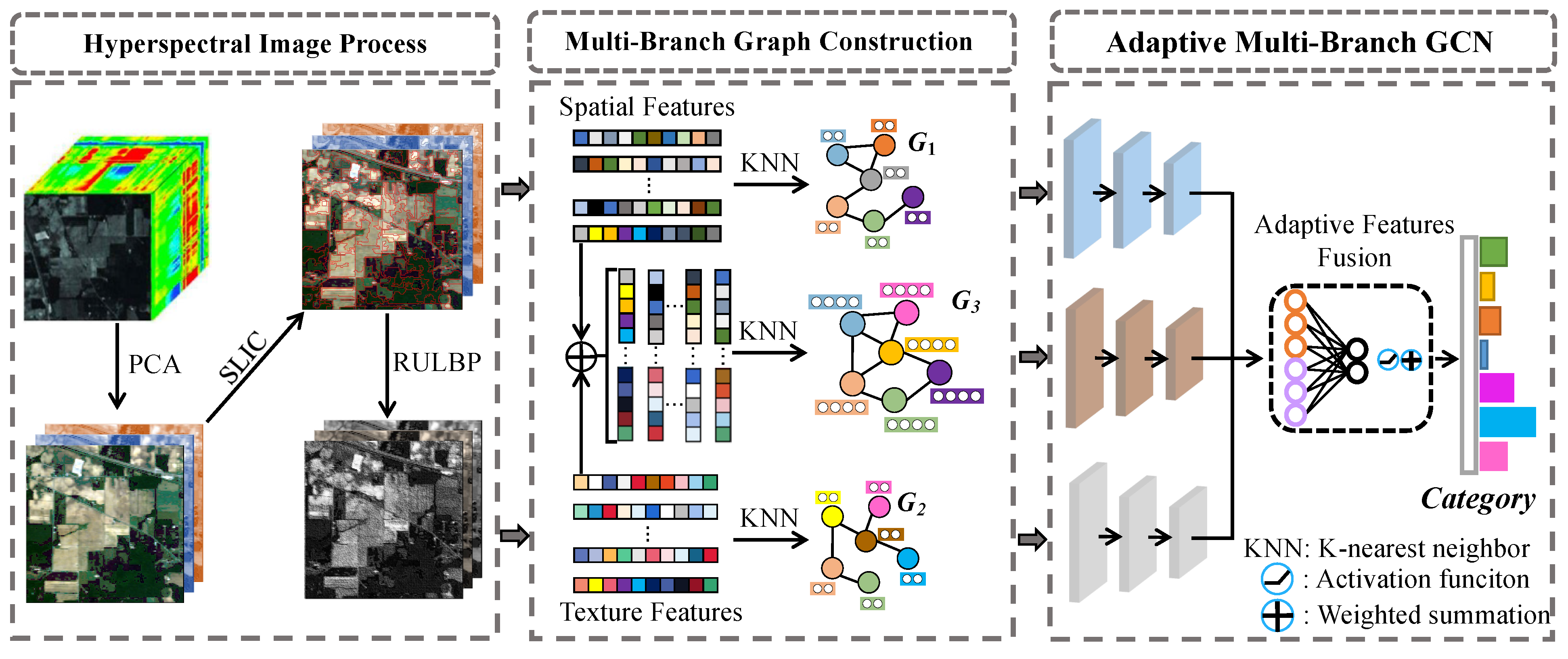
In this section, we provide a comprehensive overview of the fundamental architecture of the AMF-GCN. Figure 1 shows the overall network structure. We begin by detailing the processing of HSIs, which encompasses the extraction and fusion of spatial and textural features. Subsequently, we present the creation of multi-view features to compose separate images. Finally, we investigate the utilization of multi-branch GCNs for feature extraction and the application of an attention mechanism for feature fusion. Furthermore, we describe the detailed process of the AMF-GCN in Algorithm 1.

Algorithm 1 Learning Procedure for AMF-GCN

Input:  HSI original data $\mathbf{X}$, number of epoch T, number of superpixels N, number of graph node neighbors k 1: Obtain N superpixels by using SLIC to perform superpixel segmentation on HSI. 2: Obtain spectral features $z^s$ and texture features $z^t$ by Equation (8) and Equation (12), respectively. 3: Obtain the fused feature $z^f$ by fusing $z^s$ and $z^t$ 4: while  $epoch\le T$  do 5:    Use Equation (14) to construct adjacency matrices $A^s$, $A^t$ and $A^f$ with k-nearest neighbors for features $z^s$, $z^t$, and $z^f$. 6:    Obtain deep features $Z^S$, $Z^T$, and $Z^F$ by Equation (15) using $(z^s,A^s)$, $(z^t,A^t)$ and $(z^f,A^f)$ 7:    Obtain final feature $\mathbf{F}$ through adaptive fusion by using Equations (16) and (17). 8:    Obtain the predicted label $\mathbf{Y}$ by Equation (18). 9: end while 10: Label prediction is performed for each pixel. Output:  each pixel label

3.1. HSI Preprocessing

In this study, hyperspectral data are denoted as ${\mathbf{X}}^{\mathrm{H}}\in {\mathbb{R}}^{\mathrm{H}\times \mathrm{W}\times C}$, where H and W represent the height and width of an HSI in pixels, respectively, and C denotes the number of spectral bands in the HSI. Before proceeding with subsequent operations, we preprocessed the HSI. First, we performed principal component analysis [60] to reduce the dimensionality of the HSI. Dimensionality reduction eliminates redundant information from the original hyperspectral data. Excessive dimensions can impede the training and prediction speed of a model, thus potentially resulting in issues such as overfitting. Subsequently, we applied the simple linear iterative clustering (SLIC) [61] algorithm for superpixel segmentation. This step is essential to circumvent the substantial computational burden associated with regarding each pixel as a graph node during the composition process. The number of superpixels N obtained after the segmentation can be expressed as follows:

$$N=⌈\frac{H\times W}{\lambda }⌉,$$

(7)

where the scale parameter denoted by $\lambda$ is used to control the number of superpixels, $\lambda \ge 1$. We represent the set of all superpixels in the image as $S={\left\{S_i\right\}}_{i=1}^n$, where each $S_i={\left\{{\mathbf{x}}_j^i\right\}}_{j=1}^{{\mathbf{N}}_i}$ corresponds to the ith superpixel. Here, ${\mathbf{x}}_j^i$ represents the jth original pixel in superpixel $S_i$, and $N_i$ denotes the total number of original pixels encompassed by superpixel $S_i$. We converted all the superpixels into nodes in the topological graph. Each node $V_i$ corresponds to a superpixel $S_i$. To complete the construction of the topological map, we must acquire hyperspectral features $z^s$, texture features $z^t$, and fusion features $z^f$, in addition to an adjacency matrix representing the connection relationships between the nodes.

3.1.1. Spectral Feature Extraction

The original HSI may contain redundant information and noise, which can adversely affect feature extraction. To mitigate this issue, we employed a 1 × 1 CNN to preprocess individual pixels, and the model was shown in Figure 2. Subsequently, based on the results of the superpixel segmentation, we incorporated the spectral information of the pixels into the spectral features of the graph nodes. Specifically, the output ${\mathbf{X}}^{\left(l\right)}=\left\{{\tilde{\mathbf{x}}}_i\right\}$ obtained after the l-th convolutional layer within the node feature network structure is expressed as follows:

$${\mathbf{X}}^{\left(l\right)}=\sigma \left({\mathbf{W}}^{\left(l\right)}\ast \mathrm{BN}\left({\mathbf{X}}^{(l-1)}\right)+{\mathbf{b}}^{\left(l\right)}\right),$$

(8)

where ∗ represents the convolution operator; ${\mathbf{X}}^{(l-1)}$ signifies the input of the layer; $\mathrm{BN}(·)$ denotes batch normalization; $\sigma (·)$ is the activation function; ${\mathbf{W}}^{\left(l\right)}$ and ${\mathbf{b}}^{\left(l\right)}$ represent the learnable parameters and offsets, respectively. For a 1 × 1 convolution kernel size, the network output size remains identical to that of the input. Even after the aforementioned operation is performed, pixel-level features remain in the resulting ${\mathbf{X}}^{\left(l\right)}=\left\{{\tilde{\mathbf{x}}}_i\right\}$.

To achieve feature-level transformation while preserving the spatial information of the original image, superpixel-based feature aggregation must be performed. Let $z_k^s$ denote the spectral features of the k-th node. Hence, feature aggregation can be expressed as follows:

$${\mathbf{z}}_k^s=\frac{1}{N_k}\sum _{j=1}^{N_k}{\tilde{\mathbf{x}}}_j,$$

(9)

where $N_k$ denotes the number of pixels in the superpixel corresponding to a node. This feature aggregation method, which utilizes the average values, mitigates the effects of outlier pixels when the segmentation accuracy is compromised. By amalgamating all the node feature vectors, we obtain the spectral feature matrix $z^s=[z_1^s,z_2^s,···,z_n^s]$ for the nodes, where n denotes the number of nodes.

3.1.2. Texture Feature Extraction

To further enhance the image classification accuracy, we incorporate texture features extracted from images using the local binary pattern (LBP) technique, which are then combined with spectral features for classification. The LBP model, which was originally introduced by Ojala et al. [62,63], operates on image pixels by comparing the grayscale values of a central pixel and its neighboring pixels to form a binary bit string. Formally, the fundamental LBP operator at a specified center pixel is defined as follows:

$$LB{P}_{P,R}=\sum _{i=0}^{P-1}s\left(g_i-g_c\right)\times 2^i,$$

(10)

$$s\left(x\right)=\left\{\begin{array}{c}1,x\ge 0,\hfill \\ 0,x<0,\hfill \end{array}\right.$$

(11)

where R denotes the radius of the sampling circle; P denotes the number of sampling points situated along the circumference of the circle; $g_c$ represents the gray value attributed to the central pixel; and $g_i$ represents the gray value assigned to the ith adjacent point pixel along the sampling circle, where i ranges from 0 to $P-1$. Additionally, $s\left(x\right)$ corresponds to the threshold function employed to binarize the grayscale disparity between $g_c$ and $g_i$. In scenarios where the sampling point does not align precisely with an actual pixel, the gray level is typically estimated using standard bilinear interpolation.

By encoding all actual pixels using the LBP model expressed in Equation (10), an $m\ast n$ texture image can be encoded as an LBP-encoded image. Subsequently, a statistical frequency histogram of the encoded image is generated to construct a feature vector. To maintain rotation invariance and reduce the dimensionality of the LBP, Ojala et al. [63] proposed a rotation-invariant uniform LBP (RULBP). Through mapping, this method obtains rotation invariance and further reduces the feature dimensions. The gradient descriptor $ud$ of the RULBP is expressed as follows:

$$u{d}_{-}LB{P}_{P,R}^{riu2}=\left\{\begin{array}{c}\sum _{i=0}^{P-1}s\left(g_i-g_c\right),U\left(LB{P}_{P,R}\right)\le 2,\hfill \\ P+1,U\left(LB{P}_{P,R}\right)>2,\hfill \end{array}\right.$$

(12)

$$U\left(LB{P}_{P,R}\right)=\sum _{i=1}^{P-1}\left|s\left(g_i-g_c\right)-s\left(g_{mod(i+1,p)}-g_c\right)\right|,$$

(13)

where $U\left(LB{P}_{P,R}\right)$ is a uniformity measure that counts the number of transitions between 0 and 1 in binary.

In HSIs, every affected spectral band can be regarded as an individual grayscale image. The RULBP model was applied directly to each band, which yielded RULBP codes for every pixel. Subsequently, a statistical histogram of the central pixel image block was employed as the RULBP feature for a specific pixel. Figure 3 illustrates the process of generating RULBP features. The extracted features encompassed both primary spectral features and local texture features derived from the RULBP. This approach effectively leverages both the spatial and spectral information inherent in HSIs.

3.2. Multi-Branch Graph Construction

After obtaining the spectral feature $z^s$ and texture feature $z^t$, we used a fully connected layer to unify their lengths. Subsequently, we used the element-by-element multiplication method to fuse the two features to obtain a fused feature $z^f$. Once the feature vector $z=\{z^s,z^t,z^f\}$ is defined, connections between the edges must be established. This involves determining the adjacency matrix A based on the interactions between nodes. To maximize the preservation of the spatial information in the original image, we adopted an adjacency relationship derived from superpixels. In simpler terms, a weight of 1 was assigned to the border connecting two adjacent superpixels, whereas the weights of all other edges were set to 0 to indicate the absence of any edge connection. This can be expressed as follows:

$$A_{ij}=\left\{\begin{array}{cc}1,\hfill & {\mathrm{z}}_j\in {\mathcal{N}}_k\left({\mathrm{z}}_i\right),\hfill \\ 0,\hfill & \mathrm{otherwise},\hfill \end{array}\right.$$

(14)

where $A_{ij}$ denotes the element positioned at $(i,j)$ within the adjacency matrix A and ${\mathrm{z}}_j\in {\mathcal{N}}_k\left({\mathrm{z}}_i\right)$ represents the set of neighbors which are selected by KNN in the view that contains z. Employing the aforementioned approach, we can obtain the adjacency matrices $A=\{A^S,A^T,A^F\}$ that represent the spectral, texture, and fusion adjacency matrix. Therefore, the spectral, texture, and fusion graph can be expressed as $G^s=(z^s,A^s)$, $G^t=(z^t,A^t)$ and $G^f=(z^f,A^f)$.

3.3. Adaptive Multi-Branch GCN

3.3.1. Multi-Branch GCN

After acquiring the multi-branch features of HSIs and their corresponding adjacency matrices, we employed a GCN to aggregate adjacent node features, thereby enhancing the model’s feature extraction capabilities. As discussed previously, we introduced the GCN, and each layer of the GCN can be expressed mathematically as follows:

$$\left\{\begin{array}{c}{G}_1^s=GConv\left(G^s\right)+b_1,\hfill \\ G_1^t=GConv\left(G^t\right)+b_2,\hfill \\ G_1^f=GConv\left(G^f\right)+b_3.\hfill \end{array}\right.$$

(15)

The number of graph convolution layers was set to three. This is because employing additional graph convolution operations may result in network degradation, whereas fewer layers may not capture the full spectrum of data features effectively. After graph convolution operations were completed in the three layers, we obtained deep features, labeled as $Z^S$, $Z^T$, and $Z^F$, respectively.

Upon completing the multi-branch feature extraction, the features from each branch were fused. Furthermore, to generate the final category map, the features were remapped to the pixel level to extract the pixel-level features, thereby enabling the retrieval of category information for each individual pixel. After the dual views and their fused features were mapped back to the size of the original image based on the corresponding relationship during the superpixel segmentation, they were converted into $P^S$, $P^T$, and $P^F$.

3.3.2. Adaptive Feature Fusion

The fusion of the three features can introduce redundancy and mutual interference. To address this issue, we employed an adaptive feature fusion method. First, we consider the feature $p_s$ of any node in $G^s$ as an illustrative example. Initially, the feature was subjected to a nonlinear transformation; subsequently, an attention vector $\mathbf{q}\in {\mathbb{R}}^{h^{\prime }\times 1}$ was used to compute the attention weight ${\omega }_S^i$ as follows:

$${\omega }_S^i=q^T·tanh\left(W_S·{\left(p_S^i\right)}^T+b_S\right),$$

(16)

where ${\omega }_S\in {\mathbb{R}}^{h^{\prime }\times h}$ and $b_S\in {\mathbb{R}}^{h^{\prime }\times 1}$ represent the weight matrix and bias vector, respectively. In a similar fashion, we can calculate the attention values ${\omega }_T^i$ and ${\omega }_F^i$ for node i in the spectral graph and fusion graph, respectively. Subsequently, we normalize these values using the softmax function to derive the ultimate weights:

$${\alpha }_S^i=softmax\left({\omega }_T=S^i\right)=\frac{exp\left({\omega }_S^i\right)}{exp\left({\omega }_S^i\right)+exp\left({\omega }_T^i\right)+exp\left({\omega }_F^i\right)}.$$

(17)

A higher value of ${\alpha }_S^i$ implies greater importance for the corresponding embedding. Finally, we employed a weight vector to adaptively amalgamate the features from each component, which resulted in the ultimate fusion feature. Subsequently, the resultant final features, which contain information across multiple scales, were input into a classifier comprising a fully connected network and a softmax function to predict the category for each pixel, as depicted in Equation (18).

$$\mathbf{Y}=softmax\left(\mathrm{FC}\right(\mathrm{FC}\left(\mathbf{F}\right)\left)\right),$$

(18)

where $\mathbf{Y}$ denotes the category vector output by the network. The network employs the typically used cross-entropy loss as its loss function in classification tasks.

4. Results

4.1. HSI Datasets

To provide a fair assessment of the model’s effectiveness, it is crucial to employ a diverse dataset. This paper evaluates the model’s classification prowess using three widely recognized HSI datasets: Pavia University, Salinas, and Houston-2013. It is worth mentioning that in the experiments, the division of the training set and test set of each dataset is not fixed. Each experiment randomly selects a fixed number of sample points from the dataset as the training set and the remaining as the test set.

Pavia University dataset: The Pavia University dataset was captured by the ROSIS imaging spectrometer, operated by the German National Aeronautics and Space Administration, in 2003. The data collection took place in the city of Pavia, Italy. Subsequently, Pavia University processed the HSI obtained from the city. The dataset, after extraction, comprises dimensions of 610 × 340 × 115, incorporating 610 × 340 pixels and 115 spectral bands per pixel. The spatial resolution of the Pavia University dataset stands at 1.3 m per pixel, encompassing nine distinct labels. Figure 4 provides a pseudo-color representation of this dataset, with each color corresponding to a specific label category, and

Table 1. Detailed information of Pavia University datasets.

Pavia University Dataset
No.	Class Name	Training	Testing
1	Asphalt	30	6601
2	Meadows	30	18,619
3	Gravel	30	2069
4	Trees	30	3034
5	Painted-metal-sheets	30	1315
6	Bare-soil	30	4999
7	Bitumen	30	1300
8	Self-blocking-bricks	30	3652
9	Shadows	30	917

shows its detailed information.

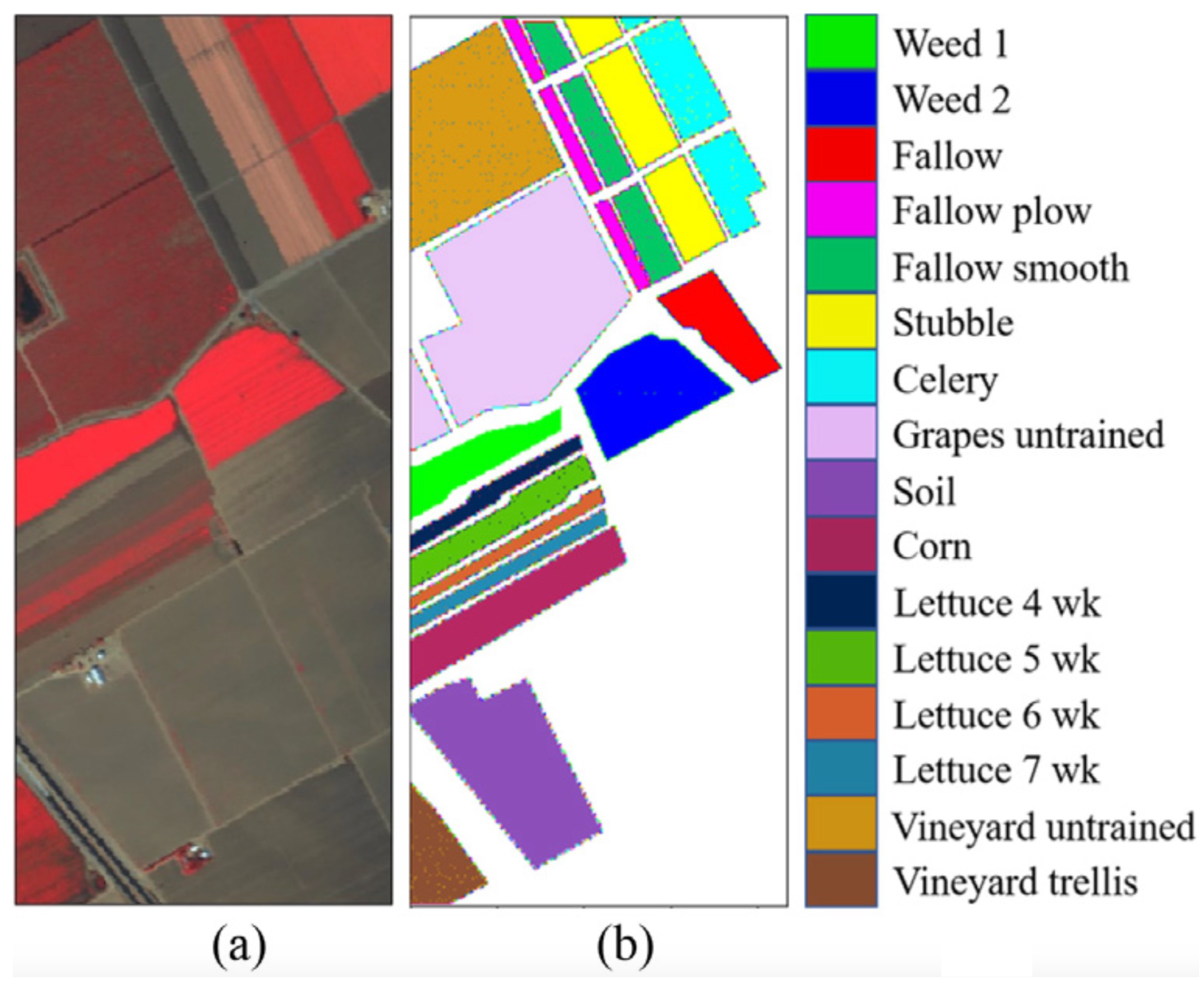
Salinas dataset: The Salinas dataset was gathered in California’s Salinas Valley back in 1992, utilizing an AVIRIS sensor. It boasts dimensions of 512 × 217 × 224, with each pixel measuring 512 × 217 and equipped with 224 spectral bands, including 20 bands related to water absorption. Spatially, the Salinas dataset has a resolution of approximately 3.7 m per pixel and incorporates 16 categories of labels. Figure 5 presents a pseudo-color image of the dataset, along with corresponding category labels represented by distinct colors, and

Table 2. Detailed information of Salinas and Houston datasets.

Salinas Dataset				Houston Dataset
No.	Class Name	Training	Testing	No.	Class Name	Training	Testing
1	Broccoli-green-weed 1	30	1979	1	Healthy-grass	30	1221
2	Broccoli-green-weed 2	30	3696	2	Stressed-grass	30	1224
3	Fallow	30	1946	3	Synthetic-grass	30	667
4	Fallow-rough-plow	30	1364	4	Trees	30	1214
5	Fallow-smooth	30	2648	5	Soil	30	1212
6	Stubble	30	3929	6	Water	30	295
7	Celery	30	3549	7	Residential	30	1238
8	Grapes-untrained	30	11,241	8	Commercial	30	1214
9	Soil-vineyard-develop	30	6137	9	Road	30	1222
10	Corn-Senesced-green-weeds	30	3248	10	Highway	30	1197
11	Lettuce-romianes-4 wk	30	1038	11	Railway	30	1205
12	Lettuce-romianes-5 wk	30	1897	12	Parking-Lot-1	30	1203
13	Lettuce-romianes-6 wk	30	886	13	Parking-Lot-2	30	439
14	Lettuce-romianes-7 wk	30	1040	14	Tennis-Court	30	398
15	Vineyard-untrained	30	7238	15	Running-Track	30	630
16	Vineyard-vertical-trellis	30	1777

shows its detailed information.

Houston dataset: It was collected by the ITRES CASI-1500 sensor at the Houston University campus in Texas, USA, and its adjacent rural areas in 2013. After deleting the noise bands, the remaining 144 valid spectral bands were used for experiments. The Houston dataset has 349 × 1905 pixels, a spatial resolution of 2.5mpp, and contains 15 land cover categories, such as tree, soil, water, healthy grass, running track, tennis court, etc. The pseudo-color images, standard classification maps, and color category labels corresponding to the Houston dataset are shown in Figure 6 and Table 2 shows its detailed information.

4.2. Setup

4.2.1. Evaluation Indices

To quantitatively analyze the advantages and disadvantages of the algorithm constructed in this article and the comparison algorithm, we use three commonly used evaluation indicators to evaluate the model proposed in this article. The following evaluation indicators can effectively evaluate the performance of the algorithm from different aspects: overall accuracy (OA), average accuracy (AA), and kappa coefficient (Kappa). The values of these three indicators are positively related to the classification effect.

(1)

Overall accuracy

Overall accuracy refers to the proportion of the number of correctly classified samples to the total number of samples after the model predicts the dataset. The higher the OA, the better the classification effect, and its mathematical definition is expressed as Equation (19).

$$OA=\frac{{\sum }_{i=1}^m{h}_{ii}}{N},$$

(19)

where N represents the total number of samples, $h_{ii}$ represents the number correctly classified into category i.

(2)

Average accuracy

Average accuracy refers to the average classification accuracy of each category, which can describe the classification difference in each category. Its mathematical definition is expressed as Equation (20).

$$AA=\frac{1}{m}\sum _{i=1}^m\frac{h_{ii}}{N_i}.$$

(20)

(3)

Kappa coefficient

The Kappa coefficient can be used to evaluate the consistency between the classification map and the reference image, can comprehensively evaluate the classification, and is defined as follows

$$\mathrm{Kappa}=\frac{N{\sum }_{\mathrm{i}=1}^m{h}_{ii}-{\sum }_{\mathrm{i}=1}^m\left(h_{i+}{h}_{+i}\right)}{N^2-{\sum }_{\mathrm{i}=1}^m\left(h_{i+}{h}_{+i}\right)},$$

(21)

where $h_{i+}$ represents the total number of samples of the i-th category, and $h_{+i}$ represents the number of samples classified as i-th. N is the total number of class samples.

4.2.2. Compared Methods

To verify the capability of the algorithm, a variety of existing advanced methods were selected for comparison in the experiment. They are ML-based algorithms: joint collaborative representation, SVM with decision fusion (JSDF) [64], and multiband compact texture units (MBCTU) [65]; CNN-based algorithms: hybrid spectral CNN (HybridSN) [66] and the diverse region-based deep CNN (DR-CNN) [67]; and algorithms based on GNN: graph sample and aggregate attention (SAGE-A) [68] and MDGCN [33]. All comparative experiments were run five times using the optimal parameters given in the article and then averaged.

4.2.3. Experimental Environment and Parameter Settings

The experiments in this article were conducted using Python version 3.9 and the PyTorch deep learning framework version 1.13. All experiments were run five times on a machine equipped with a 24 GB RTX 3090 GPU and 64 GB of RAM, with the results subsequently averaged to reduce errors. Furthermore, the Adam optimizer was employed with a learning rate set to 0.0005 for model optimization. Various parameters, such as the number of iteration steps $\left(T\right)$, k-nearest neighbor composition $\left(k\right)$, and the number of superpixels $\left(N\right)$, were adjusted to different values depending on the specific dataset under consideration. Specific information can be found in

Table 3. Hyperparameter settings applied for different datasets. T, lr, respectively, code the number of epochs and learning rate of model training. N and k, respectively, represent the number of superpixels and the value of k-nearest neighbor composition.

Dataset	T	lr	N	k
Pavia University	100	0.0005	7000	300
Salinas	200	0.0005	5000	250
Houston	200	0.0005	9000	500

.

4.3. Comparison Results

4.3.1. Quantitative Results

Table 4. Classification results of different methods in terms of per-class accuracy, OA, AA, and Kappa for Pavia University dataset (%). The optimal result is shown in bold.

Class	ML-Based Methods		CNN-Based Methods		GNN-Based Methods
	JSDF	MBCUT	HybridSN	DR-CNN	SAGE-A	MDGCN	AMF-GCN
1	82.40 ± 4.07	87.49 ± 3.99	78.05 ± 1.21	92.10 ± 3.67	96.50 ± 1.28	93.55 ± 0.37	98.86 ± 2.14
2	90.76 ± 3.74	89.11 ± 5.58	93.02 ± 1.53	96.39 ± 1.85	99.17 ± 0.62	99.25 ± 0.23	99.65 ± 0.29
3	86.71 ± 4.14	86.24 ± 4.23	84.59 ± 2.24	84.23 ± 4.21	98.26 ± 1.77	92.03 ± 0.24	97.64 ± 1.23
4	92.88 ± 2.16	90.61 ± 3.39	96.43 ± 2.91	95.26 ± 1.43	92.85 ± 2.92	83.78 ± 1.55	99.21 ± 0.36
5	100.00 ± 0.00	97.18 ± 1.28	100.00 ± 0.00	97.77 ± 1.66	97.49 ± 2.43	99.47 ± 0.09	100.00 ± 0.00
6	94.30 ± 4.55	93.25 ± 2.93	92.25 ± 0.39	90.44 ± 4.28	94.78 ± 1.62	95.26 ± 0.50	98.67 ± 0.89
7	96.62 ± 1.37	93.49 ± 2.47	99.46 ± 0.09	89.05 ± 2.85	97.92 ± 1.48	98.92 ± 1.04	90.66 ± 3.62
8	94.69 ± 3.74	84.14 ± 4.78	81.30 ± 4.71	78.49 ± 4.71	89.84 ± 4.29	94.99 ± 1.33	88.68 ± 1.07
9	99.56 ± 0.36	96.57 ± 1.22	98.89 ± 0.42	96.34 ± 1.09	98.80 ± 0.82	81.03 ± 0.49	98.51 ± 0.52
OA	90.82 ± 1.30	89.43 ± 2.14	89.99 ± 1.71	92.62 ± 1.83	96.19 ± 1.21	95.68 ± 0.22	97.45 ± 1.11
AA	93.10 ± 0.65	90.90 ± 0.89	91.67 ± 1.52	91.12 ± 1.58	96.18 ± 0.92	93.15 ± 0.28	96.77 ± 1.26
Kappa	88.02 ± 1.62	86.24 ± 2.62	86.87 ± 2.51	90.26 ± 1.72	96.24 ± 0.98	94.25 ± 0.29	96.63 ± 1.45

,

Table 5. Classification results of different methods in terms of per-class accuracy, OA, AA, and Kappa for Salinas dataset (%). The optimal result is shown in bold.

Class	ML-Based Methods		CNN-Based Methods		GNN-Based Methods
	JSDF	MBCUT	HybridSN	DR-CNN	SAGE-A	MDGCN	AMF-GCN
1	100.00 ± 0.00	99.18 ± 0.80	100.00 ± 0.00	99.40 ± 0.42	99.78 ± 0.21	99.98 ± 0.03	100.00 ± 0.00
2	100.00 ± 0.00	99.76 ± 0.33	100.00 ± 0.00	99.46 ± 0.39	100.00 ± 0.00	99.90 ± 0.28	100.00 ± 0.00
3	100.00 ± 0.00	99.13 ± 1.04	52.53 ± 5.13	98.58 ± 1.42	99.45 ± 0.35	99.80 ± 0.21	100.00 ± 0.00
4	99.93 ± 0.09	97.61 ± 0.82	100.00 ± 0.00	99.70 ± 0.17	100.00 ± 0.00	97.49 ± 2.16	99.18 ± 0.28
5	99.77 ± 0.31	96.54 ± 1.01	97.78 ± 1.47	98.90 ± 1.01	98.75 ± 1.17	97.96 ± 0.77	93.23 ± 2.59
6	100.00 + 0.00	99.74 ± 0.32	99.97 ± 0.01	99.57 ± 0.38	89.72 ± 3.62	99.10 ± 0.67	96.67 ± 1.37
7	99.99 ± 0.01	98.26 ± 1.64	99.72 ± 0.11	99.50 ± 0.42	100.00 ± 0.00	98.18 ± 1.49	99.29 ± 0.34
8	87.79 ± 4.89	81.98 ± 4.32	88.59 ± 1.28	75.59 ± 6.72	85.25 ± 5.27	92.78 ± 4.61	99.74 ± 0.13
9	99.67 ± 0.33	99.47 ± 0.51	99.95 ± 0.01	99.75 ± 0.19	95.31 ± 2.41	100.00 ± 0.00	92.98 ± 2.41
10	96.53 ± 2.55	92.21 ± 2.75	92.49 ± 1.89	94.29 ± 1.90	97.18 ± 0.82	98.31 ± 1.29	93.91 ± 1.19
11	99.71 ± 0.21	96.24 ± 2.68	99.24 ± 0.22	97.57 ± 0.91	96.36 ± 1.42	99.39 ± 0.55	99.75 ± 0.12
12	100.00 ± 0.00	98.98 ± 0.45	99.20 ± 0.17	99.99 ± 0.01	99.18 ± 0.27	99.01 ± 0.78	95.30 ± 0.99
13	100.00 ± 0.00	96.73 ± 1.66	97.49 ± 1.33	99.95 ± 0.05	97.26 ± 1.63	97.59 ± 1.32	90.15 ± 1.26
14	98.71 ± 0.72	96.50 ± 3.05	88.67 ± 5.91	98.57 ± 0.28	99.13 ± 0.46	97.92 ± 1.72	95.61 ± 2.88
15	81.86 ± 5.26	79.41 ± 5.67	87.63 ± 6.29	72.18 ± 4.97	87.23 ± 3.77	95.71 ± 4.57	96.39 ± 2.28
16	98.99 ± 0.63	96.89 ± 2.19	99.78 ± 0.19	98.45 ± 0.83	98.47 ± 0.81	98.18 ± 2.92	99.85 ± 0.06
OA	94.67 ± 0.77	92.14 ± 0.86	93.35 ± 1.26	90.35 ± 1.67	92.82 ± 1.00	97.25 ± 0.87	98.03 ± 1.02
AA	97.69 ± 0.34	95.54 ± 0.56	94.06 ± 2.41	95.72 ± 0.41	96.12 ± 0.82	98.21 ± 0.30	97.82 ± 0.58
Kappa	94.06 ± 0.85	91.25 ± 0.95	92.59 ± 1.71	89.26 ± 1.30	93.26 ± 0.76	96.94 ± 0.96	97.74 ± 1.05

and

Table 6. Classification results of different methods in terms of per-class accuracy, OA, AA, and Kappa for Houston dataset (%). The optimal result is shown in bold.

Class	ML-Based Methods		CNN-Based Methods		GNN-Based Methods
	JSDF	MBCUT	HybridSN	DR-CNN	SAGE-A	MDGCN	AMF-GCN
1	97.41 ± 1.21	92.86 ± 3.83	95.66 ± 1.17	95.62 ± 1.31	90.64 ±0.49	93.42 ± 4.25	97.51 ± 2.42
2	99.84 ± 0.25	92.18 ± 2.79	96.41 ± 2.26	96.78 ± 2.38	85.43 ± 0.34	93.67 ± 3.60	95.29 ± 1.86
3	99.57 ± 0.22	97.42 ± 1.19	99.55 ± 0.24	96.75 ± 1.40	99.25 ± 0.53	98.12 ± 1.09	99.85 ± 0.12
4	98.22 ± 2.80	90.96 ± 1.98	92.59 ± 1.67	93.41 ± 3.62	83.91 ± 2.42	95.58 ± 1.85	94.98 ± 4.13
5	100.00 ± 0.00	97.17 ± 1.29	98.68 ± 1.14	99.15 ± 0.57	99.17 ± 0.18	99.00 ± 1.30	96.12 ± 0.30
6	99.12 ± 1.09	91.78 ± 3.22	98.26 ± 0.96	93.83 ± 1.82	90.10 ± 0.20	93.28 ± 6.08	98.68 ± 0.57
7	91.32 ± 4.91	82.88 ± 3.81	82.55 ± 2.98	80.71 ± 5.81	85.04 ± 4.12	87.68 ± 4.41	94.54 ± 3.53
8	68.82 ± 6.16	71.85 ± 5.64	96.24 ± 2.21	78.32 ± 4.65	84.32 ± 2.29	80.45 ± 6.12	89.28 ± 2.01
9	69.47 ± 8.56	81.94 ± 4.25	84.35 ± 3.79	76.90 ± 3.86	75.08 ± 4.13	89.64 ± 2.26	91.12 ± 5.31
10	85.63 ± 9.32	87.31 ± 5.08	80.18 ± 3.78	81.99 ± 2.61	99.83 ± 0.09	90.06 ± 6.41	83.99 ± 1.92
11	94.51 ± 3.82	77.41 ± 6.46	89.30 ± 5.98	84.04 ± 0.88	100.00 ± 0.00	86.73 ± 3.22	94.30 ± 1.52
12	84.33 ± 5.33	86.35 ± 5.85	69.24 ± 8.55	81.92 ± 1.37	86.68 ± 3.52	89.44 ± 5.69	90.15 ± 0.87
13	98.10 ± 1.28	85.58 ± 5.35	93.80 ± 4.27	86.54 ± 4.17	91.30 ± 1.23	92.78 ± 4.45	88.04 ± 3.98
14	100.00 ± 0.00	96.85 ± 1.85	99.21 ± 0.19	99.31 ± 0.16	100.00 ± 0.00	99.43 ± 0.97	100.00 ± 0.00
15	99.86 ± 0.36	92.27 ± 3.32	99.73 ± 0.14	99.60 ± 0.29	100.00 ± 0.00	96.27 ± 1.72	96.92 ± 1.23
OA	90.51 ± 0.95	87.07 ± 1.12	87.85 ± 1.36	88.08 ± 1.47	89.58 ± 2.39	91.40 ± 0.92	93.02 ± 0.49
AA	92.46 ± 0.75	89.32 ± 1.08	89.93 ± 0.78	89.66 ± 1.17	90.18 ± 0.11	92.37 ± 0.89	93.84 ± 0.34
Kappa	89.74 ± 1.03	86.01 ± 1.21	86.87 ± 1.94	87.10 ± 0.99	87.52 ± 1.26	90.70 ± 1.00	92.83 ± 0.53

present the classification accuracy for each category and the results of three evaluation indices for various methods on the Pavia University, Salinas, and Houston datasets. AMF-GCN consistently achieved the highest classification results across all datasets. In the three datasets, the OA reached remarkable levels of 91% and 92%, respectively.

As observed in Table 4, the proposed AMF-GCN method demonstrates clear superiority over GNN-based approaches and all other classifiers in the Pavia dataset. AMF-GCN notably outperforms SAGE-A and MDGCN by 1.26% and 1.77% in terms of OA, respectively. When compared to CNN-based methods, AMF-GCN exhibits a remarkable 4.83% and 7.46% OA advantage. Although the Salinas dataset contains numerous categories and a substantial amount of data, the AMF-GCN method presented in this article still achieved the highest OA and kappa accuracy. As evident from Table 5, the ML-based method delivered impressive results. The 3DCNN method leverages three-dimensional convolutional kernels to concurrently capture the spatial–spectral features of HSI, resulting in enhanced classification accuracy. However, these methods tend to overlook node features within the image and may not emphasize important information. Consequently, AMF-GCN achieves significant gains in the range of 5.89–8.48% in Kappa on the Salinas dataset. In the classification of broccoli green weed1, broccoli green weed2, and fallow species, AMF-GCN achieved 100% classification results. In contrast to the previous two datasets, the Houston dataset features more dispersed labeled areas with smaller scales. In such scenarios, relying solely on shallow spectral information from the HSI may not suffice for intricate and fine-grained classification. SAGE-A and MDGCN achieved OA of 89.58% and 91.40%, respectively, which, although respectable, did not reach exceptional accuracy. However, AMF-GCN achieved an impressive OA of 93.02%, underscoring the benefit of extracting and fusing multiple features to enhance network performance.

4.3.2. Visual Results

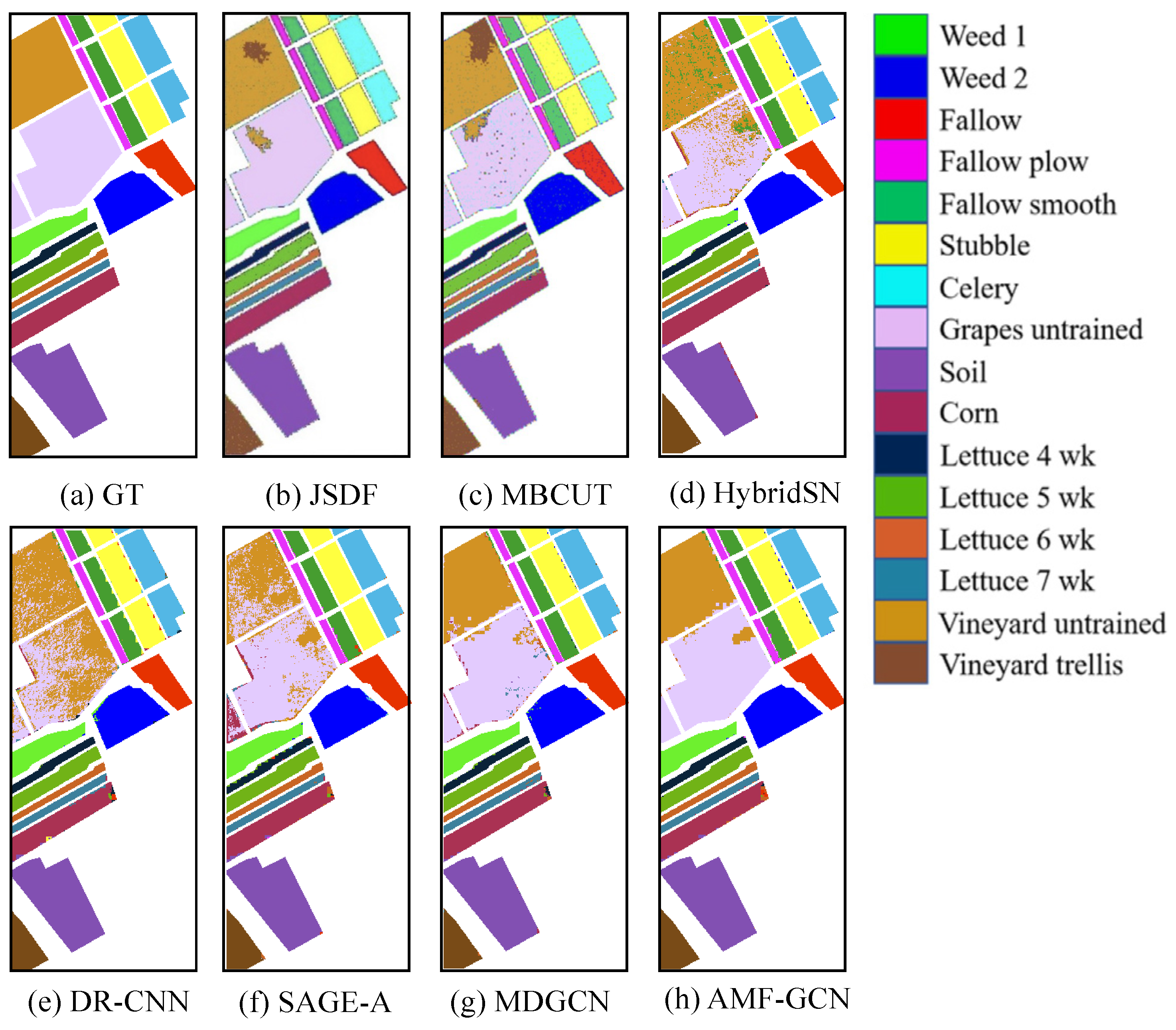
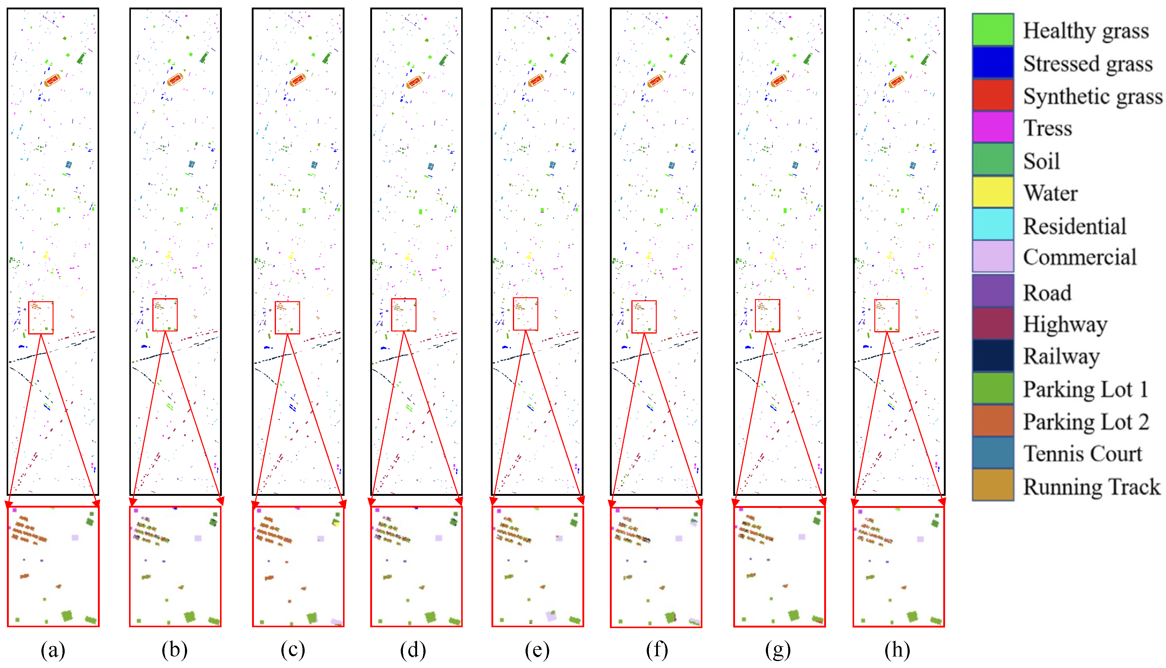
To facilitate a more intuitive comparison of the classification accuracy among different algorithms, this experiment includes visualizations of the classification results for three datasets: Pavia, Salinas, and Houston, as depicted in Figure 7, Figure 8 and Figure 9. An immediate observation is that the ground object classification map generated by AMF-GCN exhibits the most impressive display, with fewer instances of misclassification and a smoother appearance compared to the two convolutional neural network methods. Furthermore, it is noticeable that on the Pavia and Salinas datasets, the ML-based method excels in classifying certain category blocks but introduces larger errors in certain neighborhoods, particularly involving self-blocking bricks and trees. This suggests that the ML-based method may struggle with complex scenarios involving smaller blocks. However, the approach presented in this chapter demonstrates competence not only in handling complex situations within larger classification blocks but also in dealing effectively with intricate scenarios within smaller classification blocks. When compared to the CNN-based method, it is evident that both methods perform admirably when utilizing neighborhood information. Nonetheless, it is worth noting that at the boundaries, the CNN-based method lags behind AMF-GCN, indicating that AMF-GCN offers greater flexibility than CNN-based methods. In conclusion, compared to other methods, this approach leverages the attention mechanism to make more effective use of spatial information. It displays very few instances of misclassification points internally, and simultaneously, it accurately captures details within the black boxes, outperforming other methods by a considerable margin. This further underscores the distinct advantages of the attention mechanism in harnessing spatial information.

4.4. Parameter Analysis

In this section, we delve into a detailed investigation of the impacts of k and N. The experiments systematically vary the sizes of k and N across the dataset scales, as illustrated in Figure 10, showcasing the experimental results under different parameter combinations. Specifically, k ranges from 100 to 600 at intervals of 100 for the Pavia University and Houston datasets, and from 100 to 350 at intervals of 50 for the Salinas dataset. The resulting surface reflects that using a smaller number of edges to construct the graph during information aggregation may overlook important neighbor nodes containing crucial information. In HSI, correlation information between pixels at both short and long distances can contribute to improved classification results. Therefore, preserving the integrity of the graph data is pivotal for model learning. However, it is evident that excessively large k values lead to reduced model accuracy on all three datasets, indicating that an excessive number of neighbor nodes can introduce noise. Consequently, selecting an appropriate number of neighbor nodes is of paramount importance.

Furthermore, the number of superpixels inversely affects the segmentation map size obtained. Smaller numbers of superpixels retain larger objects while suppressing more noise, whereas larger numbers of superpixels yield smaller segmentation maps, preserving smaller objects but potentially introducing more noise. To analyze the impact of the number of superpixel blocks on classification results, the experiment sets N to range from 1000 to 11,000 and tests the classification accuracy of AMF-GCN on each dataset. As depicted in Figure 10, the classification accuracy on the Pavia University dataset demonstrates an upward trend as N increases. This is attributed to the larger category scale within the dataset, with increased segmentation contributing to overall accuracy improvement. The pixel segmentation process effectively suppresses classification map noise resulting from misclassification. However, it is important to note that this upward trend may not persist indefinitely. To avoid excessively smooth classification maps, the number of segmentations for different datasets was set to the most appropriate value during the experiments in this chapter.

4.5. Ablation Study

To comprehensively evaluate the AMF-GCN algorithm introduced in this study, this section conducts a series of rigorous ablation experiments. Firstly, AMF-GCN comprises three branches, with each branch receiving inputs of spectral features, texture features, and fusion features. In an effort to dissect the specific contributions of these three types of features, we assessed their individual classification accuracy on the Pavia University, Salinas, and Houston datasets. Secondly, we investigated the influence of the attention-based feature fusion mechanism by testing the network’s accuracy without its inclusion. The results of these experiments are presented in

Table 7. Classification results of different methods in terms of per-class accuracy, OA, AA, and Kappa for the Houston dataset (%). The optimal result is shown in bold.

Pavia University
No.	Spectral Feature	Texture Feature	Fusion Feature	Attention Fusion	OA	AA	Kappa
1	✔				95.74 ± 0.74	93.33 ± 1.19	94.36 ± 0.98
2		✔			95.87 ± 0.48	94.58 ± 1.56	95.18 ± 0.64
3			✔		96.39 ± 0.96	93.98 ± 1.10	95.01 ± 0.84
4	✔	✔			96.49 ± 0.68	94.29 ± 0.71	95.37 ± 0.88
5	✔	✔	✔		96.59 ± 0.65	94.04 ± 1.14	95.11 ± 0.84
6	✔	✔	✔	✔	97.45 ± 1.11	96.77 ± 1.26	96.63 ± 1.45
Salinas
	Spectral Feature	Texture Feature	Fusion Feature	Attention Fusion	OA	AA	Kappa
1	✔				94.49 ± 1.17	95.38 ± 1.40	94.10 ± 1.29
2		✔			94.45 ± 3.01	95.14 ± 0.90	94.72 ± 3.35
3			✔		96.37 ± 1.27	95.67 ± 0.65	96.14 ± 0.44
4	✔	✔			96.42 ± 1.97	95.65 ± 0.41	96.02 ± 0.22
5	✔	✔	✔		96.98 ± 0.51	96.54 ± 0.27	96.64 ± 0.56
6	✔	✔	✔	✔	98.03 ± 1.02	97.82 ± 0.58	97.74 ± 1.05
Houston
	Spectral Feature	Texture Feature	Fusion Feature	Attention Fusion	OA	AA	Kappa
1	✔				91.59 ± 1.22	92.88 ± 0.89	91.19 ± 1.32
2		✔			90.33 ± 0.11	91.50 ± 0.12	90.17 ± 0.12
3			✔		92.28 ± 0.47	92.18 ± 0.56	91.14 ± 0.80
4	✔	✔			92.16 ± 0.72	92.26 ± 0.43	91.01 ± 0.78
5	✔	✔	✔		92.66 ± 0.59	92.36 ± 0.98	91.26 ± 0.64
6	✔	✔	✔	✔	93.02 ± 0.49	93.84 ± 0.34	92.83 ± 0.53

.

Upon reviewing the table, it becomes evident that the absence of any feature results in a decline in overall classification accuracy. On the Salinas dataset, the network that fused spatial–spectral and texture features outperformed individual features by 1.93% and 1.97%, respectively. This underscores the synergy between texture and spectral information extracted from multiple perspectives, ultimately enhancing classification performance. Furthermore, the omission of the attention mechanism led to reduced classification results, with an OA drop of 0.86%, 0.86%, and 0.36% for the three datasets, respectively. Otherwise, multi-feature fusion variant 5 exhibited 0.20%, 0.61%, and 0.38% greater overall accuracy on the three datasets compared to variant 3, which utilized exclusively fused representations. This highlights the significance of incorporating an attention-based feature fusion mechanism, enabling the model to assign varying degrees of importance to different features and thereby improving classification outcomes.

5. Discussion

5.1. Comparison with Various Graph-Based Models

To further demonstrate the advantages of our model, we compare it with advanced methods in recent years on the Pavia University and Salinas datasets, namely MSAGE-Cal [52], MSSUG [53], SSG [50], SSPGAT [51], and MARP [18], respectively. Several algorithms mentioned above incorporate multi-feature fusion techniques. For instance, SSPGAT employs the graph attention network to seamlessly merge pixel and superpixel features, enhancing hyperspectral classification. MSAGE-Cal integrates multi-scale and global information from the graph, whereas MSSUG creates multilevel graphs by combining adjacent regions in HSIs, capturing spatial topologies in a multi-scale hierarchical fashion. Additionally, MARP discerns the importance weights of various hop neighborhoods and aggregates nodes selectively and automatically. From

Table 8. Classification results of different methods in terms OA, AA, and Kappa for Pavia University and Salinas datasets (%). The optimal result is shown in bold.

Datasets	Matrix	MSAGE-Cal	MSSUG	SSG	SSPGAT	MARP	AMF-GCN
		JSTARS 2021	TGRS 2022	RS 2021	IGARSS 2023	ESWA 2023	Ours
Pavia University	OA	96.39 ± 1.27	92.06 ± 1.01	94.82 ± 0.94	96.35 ± 0.74	97.09 ± 1.24	97.45 ± 1.11
	AA	96.22 ± 1.84	97.65 ± 0.26	94.24 ± 0.63	95.88 ± 1.09	97.12 ± 1.35	96.77 ± 1.26
	Kappa	95.24 ± 1.59	89.81 ± 1.26	94.69 ± 0.35	95.59 ± 0.67	96.12 ± 0.58	96.63 ± 1.45
Salinas	OA	97.61 ± 1.19	97.99 ± 1.14	97.64 ± 0.58	97.58 ± 0.84	97.81 ± 0.80	98.03 ± 1.02
	AA	96.94 ± 0.98	97.87 ± 0.85	96.82 ± 1.12	97.39 ± 0.91	98.04 ± 0.29	97.82 ± 0.58
	Kappa	97.34 ± 0.87	97.43±0.79	97.15 ± 1.09	97.25 ± 0.78	97.12 ± 0.55	97.74 ± 1.05

, it is evident that AMF-GCN consistently achieves optimal performance across various evaluation metrics. In the case of the Pavia dataset, the OA accuracy of AMF-GCN surpasses other models MARP, SSPGAT, SSG, MSSUG, and MSAGE-Cal by 0.36%, 1.1%, 2.63%, 5.39%, and 1.06%, respectively. When considering the Salinas dataset, the accuracy of AMF-GCN outperforms other models by 0.22%, 0.45%, 0.39%, 0.04%, and 0.42%, respectively. There are two key factors contributing to the superior accuracy of AMF-GCN. Firstly, AMF-GCN effectively aggregates multi-view features, leveraging their complementary information. Additionally, unlike other models that simply fuse features, AMF-GCN employs an attention-based feature fusion mechanism, adaptively selecting features and reducing redundancy to a significant extent.

5.2. Impact of the Number of Training Samples

The number of training samples plays a crucial role in determining the classification performance of a network. Generally, a higher number of samples correlates positively with improved model performance. Increasing the number of samples allows the model to more accurately learn data features and reduces the risk of network overfitting. To assess the impact of sample size on AMF-GCN and other methods, we varied the number of training samples for each class in the three datasets, ranging from 5 to 30 with intervals of 5 increments. Figure 11 presents the overall classification accuracy achieved by four methods (HybridSN, SAGE-A, MDGCN, and AMF-GCN) on the three datasets. It is evident that increasing the number of samples enhances the classification accuracy of each method. This underscores the significance of sample size in influencing classification results. Notably, AFM-GCN outperforms other methods in classification accuracy, demonstrating its robustness and advantages, especially in scenarios with limited samples. These advantages are attributed to its ability to extract multi-view features and the incorporation of modules such as superpixel segmentation and attention-based feature fusion. In contrast, HybridSN exhibits the lowest classification results, primarily due to its heavy reliance on training data. GCN performs better than HybridSN with a small number of samples because the relationship features obtained through the graph structure help mitigate the challenge of having an insufficient number of HSI training samples. GCN effectively captures global relationships among nodes in the graph data, and classification tasks are performed based on these relationship features.

5.3. Influence of Different Texture Feature Extraction Methods

We are already aware of the significant role that texture information in HSI plays in complementing and enhancing the accuracy of downstream tasks. The effectiveness of texture information extraction also directly influences the quality of the extracted features. Consequently, this section delves into the impact of various texture feature extraction methods on our experiments, with the results presented in

Table 9. OA $(\%)$ indices of AMF-GCN with different texture feature extraction on four datasets. The methods used are extended morphological profiles (EMP), local binary pattern (LBP), and rotation-invariant uniform LBP (RULBP).

Dataset	EMP	LBP	RULBP
Pavia University	96.02 ± 2.21	96.89 ± 1.05	97.45 ± 1.11
Salinas	96.18 ± 1.60	97.24 ± 1.33	98.03 ± 1.02
Houston	91.11 ± 0.97	91.85 ± 0.72	93.02 ± 0.49

. The chosen texture feature extraction algorithms encompass extended morphological profile (EMP) [14], LBP, and RULBP. The EMP represents a structural approach that characterizes texture primitives and their spatial arrangements while reducing noise through morphological operations. The results reveal that the EMP algorithm successfully eliminates misclassified patches within ground objects via morphological transformations, achieving commendable accuracy. However, it falls slightly behind the LBP-based method. Notably, RULBP emerges as the top-performing approach, outperforming other methods by 1.43%/0.56%, 1.85%/0.79%, and 1.92%/1.17% on the Pavia University, Salinas, and Houston datasets, showcasing its effectiveness.

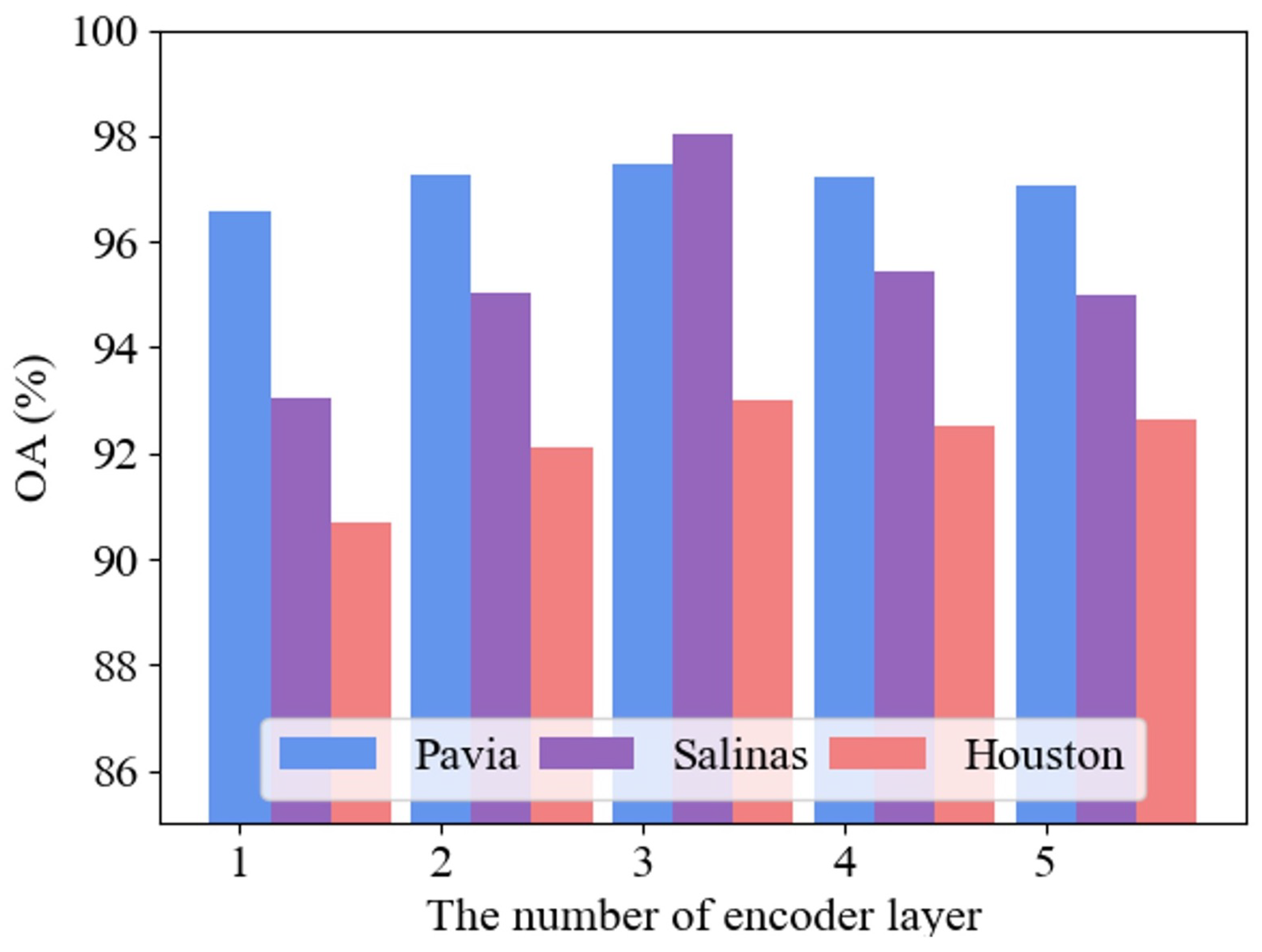
5.4. Influence of the Number of Encoder Layer

To some extent, the performance of a neural network is positively correlated with the number of layers it possesses. However, increasing the number of layers can lead to issues like gradient vanishing or explosion, which can hinder convergence, slow down training, and even degrade performance. Consequently, determining the appropriate number of network layers must be guided by the specific problem and dataset feature. To evaluate the impact of network depth on AMF-CGN, this section conducts experiments with different depths, setting the number of network layers to 1, 2, 3, 4, and 5, and assessing AMF-CGN’s performance under these various depths. The results are presented in Figure 12. Upon examining the results for the Pavia University dataset, it is evident that the performance is quite similar when the network depth is 2 and 3. This is because deeper GCN layers tend to produce smoother classification maps. Given that the Pavia University dataset consists of relatively large-scale ground object categories, this smoothing effect does not significantly impact its performance. However, deeper network layers enable the model to extract richer features. For the Salinas and Houston datasets, optimal performance is achieved with a network depth of 3. Taking into account the network’s performance across all three datasets, a network depth of 3 is selected for this chapter.

5.5. Complete Image Visualization

To further validate the consistency and robustness of our classification model, we applied it to fully test unseen images containing both labeled reference samples and unlabeled background pixels. As shown in Figure 13, we compare our model against three graph-based approaches. Our model demonstrates the best performance for classes like grape untrained and vineyard untrained, exhibiting minimal impact from noisy backgrounds. This can be attributed to the incorporation of texture information, which enhances the model’s feature extraction abilities and robustness.

6. Conclusions

In this paper, we introduce a novel HSI classification approach known as AMF-GCN. This method involves the extraction and fusion of spectral and texture features to create multi-view features. It utilizes three separate branches for graph convolution operations to consolidate node information and employs an attention mechanism-based feature fusion technique for adaptive feature fusion. Extensive ablation experiments and discussions are conducted to thoroughly evaluate the proposed method. The results, obtained from experiments on three commonly used datasets, demonstrate the efficacy and advantages of the proposed AMF-GCN. They also demonstrate that AMF-GCN outperforms all comparative methods and achieves outstanding performance.

However, there are two limitations to our model. Firstly, constructing multiple views comes at the cost of computational efficiency. Secondly, our superpixel division method is static and only utilizes shallow spectral information. Going forward, we aim to explore dynamic superpixel generation techniques that can co-evolve with model training for even stronger performance. Furthermore, in future work, we plan to explore unsupervised learning techniques for clustering tasks on HSI and delve deeper into the spatial autocorrelation aspects of HSI.

References

- He, L.; Li, J.; Liu, C.; Li, S. Recent advances on spectral-spatial hyperspectral image classification: An overview and new guidelines. IEEE Trans. Geosci. Remote Sens. 2018, 56, 1579–1597. [Google Scholar] [CrossRef]
- Chen, Y.; Zhao, X.; Jia, X. Spectral-spatial classification of hyperspectral data based on deep belief network. IEEE J. Sel. Top. Appl. Earth Obs. Remote Sens. 2015, 8, 2381–2392. [Google Scholar] [CrossRef]
- Kruse, F. Identification and mapping of minerals in drill core using hyperspectral image analysis of infrared reflectance spectra. Int. J. Remote Sens. 1996, 17, 1623–1632. [Google Scholar] [CrossRef]
- Liu, Z.; Guan, R.; Hu, J.; Chen, W.; Li, X. Remote Sensing Scene Data Generation Using Element Geometric Transformation and GAN-Based Texture Synthesis. Appl. Sci. 2022, 12, 3972. [Google Scholar] [CrossRef]
- Guan, R.; Li, Z.; Li, T.; Li, X.; Yang, J.; Chen, W. Classification of Heterogeneous Mining Areas Based on ResCapsNet and Gaofen-5 Imagery. Remote Sens. 2022, 14, 3216. [Google Scholar] [CrossRef]
- Peng, J.; Li, L.; Tang, Y.Y. Maximum Likelihood Estimation-Based Joint Sparse Representation for the Classification of Hyperspectral Remote Sensing Images. IEEE Trans. Neural Netw. Learn. Syst. 2019, 30, 1790–1802. [Google Scholar] [CrossRef]
- Chen, W.; Ouyang, S.; Yang, J.; Li, X.; Zhou, G.; Wang, L. JAGAN: A Framework for Complex Land Cover Classification Using Gaofen-5 AHSI Images. IEEE J. Sel. Top. Appl. Earth Observ. Remote Sens. 2022, 15, 1591–1603. [Google Scholar] [CrossRef]
- Bioucas-Dias, J.; Plaza, A.; Camps-Valls, G.; Scheunders, P.; Nasrabadi, N.; Chanussot, J. Hyperspectral remote sensing data analysis and future challenges. IEEE Geosci. Remote Sens. Mag. 2013, 1, 6–36. [Google Scholar] [CrossRef]
- Audebert, N.; Le, B.; Lefevre, S. Deep learning for classification of hyperspectral data: A comparative review. IEEE Geosci. Remote Sens. Mag. 2019, 7, 159–173. [Google Scholar] [CrossRef]
- Ma, L.; Crawford, M.M.; Tian, J. Local manifold learning-based k-nearest-neighbor for hyperspectral image classification. IEEE Trans. Geosci. Remote Sens. 2010, 48, 4099–4109. [Google Scholar] [CrossRef]
- Melgani, F.; Bruzzone, L. Classification of hyperspectral remote sensing images with support vector machines. IEEE Trans. Geosci. Remote Sens. 2004, 42, 1778–1790. [Google Scholar] [CrossRef]
- Ham, J.; Chen, Y.; Crawford, M.M.; Ghosh, J. Investigation of the random forest framework for classification of hyperspectral data. IEEE Trans. Geosci. Remote Sens. 2005, 43, 492–501. [Google Scholar] [CrossRef]
- Gu, Y.; Liu, T.; Jia, X.; Benediktsson, J.A.; Chanussot, J. Nonlinear multiple kernel learning with multiple-structure-element extended morphological profiles for hyperspectral image classification. IEEE Trans. Geosci. Remote Sens. 2016, 54, 3235–3247. [Google Scholar] [CrossRef]
- Benediktsson, J.A.; Palmason, J.A.; Sveinsson, J.R. Classification of hyperspectral data from urban areas based on extended morphological profiles. IEEE Trans. Geosci. Remote Sens. 2005, 43, 480–491. [Google Scholar] [CrossRef]
- Li, J.J.; Xi, B.B.; Li, Y.S.; Du, Q.; Wang, K.Y. Hyperspectral Classification Based on Texture Feature Enhancement and Deep Belief Networks. Remote Sens. 2018, 10, 396. [Google Scholar] [CrossRef]
- Bhatti, U.A.; Yu, Z.; Chanussot, J.; Zeeshan, Z.; Yuan, L.; Luo, W.; Nawaz, S.A.; Bhatti, M.A.; Ain, Q.U.; Mehmood, A. Local Similarity-Based Spatial–Spectral Fusion Hyperspectral Image Classification with Deep CNN and Gabor Filtering. IEEE Trans. Geosci. Remote Sens. 2021, 60, 5514215. [Google Scholar] [CrossRef]
- Ding, Y.; Zhang, Z.; Zhao, X.; Hong, D.; Cai, W.; Yu, C.; Yang, N.; Cai, W. Multi-feature fusion: Graph neural network and CNN combining for hyperspectral image classification. Neurocomputing 2022, 501, 246–257. [Google Scholar] [CrossRef]
- Zhang, Z.; Ding, Y.; Zhao, X.; Siye, L.; Yang, N.; Cai, Y.; Zhan, Y. Multireceptive field: An adaptive path aggregation graph neural framework for hyperspectral image classification. Expert Syst. Appl. 2023, 217, 119508. [Google Scholar] [CrossRef]
- Ding, Y.; Zhao, X.; Zhang, Z.; Cai, W.; Yang, N.; Zhan, Y. Semi-supervised locality preserving dense graph neural network with ARMA filters and context-aware learning for hyperspectral image classification. IEEE Trans. Geosci. Remote Sens. 2021, 60, 5511812. [Google Scholar] [CrossRef]
- Yang, X.; Ye, Y.; Li, X.; Lau, R.Y.K.; Zhang, X.; Huang, X. Hyperspectral Image Classification with Deep Learning Models. IEEE Trans. Geosci. Remote Sens. 2018, 56, 5408–5423. [Google Scholar] [CrossRef]
- Fang, L.; Liu, Z.; Song, W. Deep hashing neural networks for hyperspectral image feature extraction. IEEE Geosci. Remote. Sens. Lett. 2019, 16, 1412–1416. [Google Scholar] [CrossRef]
- Chen, Y.; Lin, Z.; Zhao, X.; Wang, G.; Gu, Y. Deep learning-based classification of hyperspectral data. IEEE J. Sel. Top. Appl. Earth Obs. Remote Sens. 2014, 7, 2094–2107. [Google Scholar] [CrossRef]
- Mou, L.; Ghamisi, P.; Zhu, X.X. Deep recurrent neural networks for hyperspectral image classification. IEEE Trans. Geosci. Remote Sens. 2017, 55, 3639–3655. [Google Scholar] [CrossRef]
- He, J.; Zhao, L.; Yang, H. HSI-BERT: Hyperspectral image classification using the bidirectional encoder representation from transformers. IEEE Trans. Geosci. Remote Sens 2019, 58, 165–178. [Google Scholar] [CrossRef]
- Hong, D.; Han, Z.; Yao, J. SpectralFormer: Rethinking hyperspectral image classification with transformers. IEEE Trans. Geosci. Remote Sens. 2021, 60, 1–15. [Google Scholar] [CrossRef]
- Li, X.; Ding, M.; Pižurica, A. Deep Feature Fusion via Two-Stream Convolutional Neural Network for Hyperspectral Image Classification. IEEE Trans. Geosci. Remote Sens. 2020, 58, 2615–2629. [Google Scholar] [CrossRef]
- Yu, S.; Jia, S.; Xu, C. Convolutional neural networks for hyperspectral image classification. Neurocomputing 2017, 219, 88–98. [Google Scholar] [CrossRef]
- Jia, P.; Zhang, M.; Yu, W.; Shen, F.; Shen, Y. Convolutional neural network based classification for hyperspectral data. In Proceedings of the IEEE International Geoscience and Remote Sensing Symposium (IGARSS), Beijing, China, 10–15 July 2016; pp. 5075–5078. [Google Scholar]
- Makantasis, K.; Karantzalos, K.; Doulamis, A.; Doulamis, N. Deep Supervised Learning for Hyperspectral Data Classification through Convolutional Neural Networks. In Proceedings of the IEEE International Geoscience and Remote Sensing Symposium (IGARSS), Milan, Italy, 26–31 July 2015; pp. 4959–4962. [Google Scholar]
- Ma, X.; Wang, H.; Geng, J. Spectral–spatial classification of hyperspectral image based on deep auto-encoder. IEEE J. Sel. Top. Appl. Earth Obs. Remote Sens. 2016, 9, 4073–4085. [Google Scholar] [CrossRef]
- Lee, H.; Kwon, H. Going deeper with contextual CNN for hyperspectral image classification. IEEE Trans. Image Process. 2017, 26, 4843–4855. [Google Scholar] [CrossRef]
- Zhu, M.; Jiao, L.; Liu, F.; Yang, S.; Wang, J. Residual spectral-spatial attention network for hyperspectral image classification. IEEE Trans. Geosci. Remote Sens. 2021, 59, 449–462. [Google Scholar] [CrossRef]
- Wan, S.; Gong, C.; Zhong, P.; Du, B.; Zhang, L.; Yang, J. Multiscale dynamic graph convolutional network for hyperspectral image classification. IEEE Trans. Geosci. Remote Sens. 2019, 58, 3162–3177. [Google Scholar] [CrossRef]
- Liang, L.; Zhang, Y.; Zhang, S.; Li, J.; Plaza, A.; Kang, X. Fast Hyperspectral Image Classification Combining Transformers and SimAM-based CNNs. IEEE Trans. Geosci. Remote Sens. 2023, 61, 5522219. [Google Scholar] [CrossRef]
- Liu, W.; Liu, B.; He, P.; Hu, Q.; Gao, K.; Li, H. Masked Graph Convolutional Network for Small Sample Classification of Hyperspectral Images. Remote Sens. 2023, 15, 1869. [Google Scholar] [CrossRef]
- Xu, Z.; Su, C.; Wang, S.; Zhang, X. Local and Global Spectral Features for Hyperspectral Image Classification. Remote Sens. 2023, 15, 1803. [Google Scholar] [CrossRef]
- Wu, Z.; Pan, S.; Chen, F.; Long, G.; Zhang, C.; Yu, P.S. A Comprehensive Survey on Graph Neural Networks. IEEE Trans. Neural Netw. Learn. Syst. 2021, 32, 4–24. [Google Scholar] [CrossRef] [PubMed]
- Qin, A.; Shang, Z.; Tian, J.; Wang, Y.; Zhang, T.; Tang, Y. Spectral–spatial graph convolutional networks for semisupervised hyperspectral image classification. IEEE Geosci. Remote Sens. Lett. 2018, 16, 241–245. [Google Scholar] [CrossRef]
- Mou, L.; Lu, X.; Li, X.; Zhu, X.X. Nonlocal graph convolutional networks for hyperspectral image classification. IEEE Trans. Geosci. Remote Sens. 2020, 58, 8246–8257. [Google Scholar] [CrossRef]
- Zhang, S.; Tong, H.; Xu, J.; Maciejewski, R. Graph convolutional networks: A comprehensive review. Comput. Soc. Netw. 2019, 6, 11. [Google Scholar] [CrossRef]
- Liu, Y.; Tu, W.; Zhou, S.; Liu, X.; Song, L.; Yang, X.; Zhu, E. Deep graph clustering via dual correlation reduction. In Proceedings of the AAAI Conference on Artificial Intelligence, Virtual, 22 February–1 March 2022; Volume 36, pp. 7603–7611. [Google Scholar]
- Tu, W.; Zhou, S.; Liu, X.; Ge, C.; Cai, Z.; Liu, Y. Hierarchically Contrastive Hard Sample Mining for Graph Self-Supervised Pretraining. IEEE Trans. N eural Netw. Learn. Syst. 2023; early access. [Google Scholar]
- He, X.; Chen, Y.; Ghamisi, P. Dual Graph Convolutional Network for Hyperspectral Image Classification with Limited Training Samples. IEEE Trans. Geosci. Remote Sens. 2021, 60, 5502418. [Google Scholar] [CrossRef]
- Hong, D.; Gao, L.; Yao, J.; Zhang, B.; Plaza, A.; Chanussot, J. Graph Convolutional Networks for Hyperspectral Image Classification. IEEE Trans. Geosci. Remote Sens. 2021, 59, 5966–5978. [Google Scholar] [CrossRef]
- Liu, Q.; Xiao, L.; Yang, J.; Wei, Z. CNN-Enhanced Graph Convolutional Network With Pixel- and Superpixel-Level Feature Fusion for Hyperspectral Image Classification. IEEE Trans. Geosci. Remote Sens. 2021, 59, 8657–8671. [Google Scholar] [CrossRef]
- Yang, B.; Cao, F.; Ye, H. A Novel Method for Hyperspectral Image Classification: Deep Network with Adaptive Graph Structure Integration. IEEE Trans. Geosci. Remote Sens. 2022, 60, 5523512. [Google Scholar] [CrossRef]
- Wang, J.; Sun, J.; Zhang, E.; Zhang, T.; Yu, K.; Peng, J. Hyperspectral image classification via deep network with attention mechanism and multigroup strategy. Expert Syst. Appl. 2023, 224, 119904. [Google Scholar] [CrossRef]
- Ding, Y.; Zhang, Z.-L.; Zhao, X.-F.; Cai, W.; He, F.; Cai, Y.-M.; Cai, W. Deep hybrid: Multi-graph neural network collaboration for hyperspectral image classification. Def. Technol. 2022, 23, 164–176. [Google Scholar]
- Bai, J.; Shi, W.; Xiao, Z.; Regan, A.C.; Ali, T.A.A.; Zhu, Y.; Zhang, R.; Jiao, L. Hyperspectral Image Classification Based on Superpixel Feature Subdivision and Adaptive Graph Structure. IEEE Trans. Geosci. Remote Sens. 2022, 60, 5524415. [Google Scholar] [CrossRef]
- Zhao, Y.; Yan, F. Hyperspectral Image Classification Based on Sparse Superpixel Graph. Remote Sens. 2021, 13, 3592. [Google Scholar] [CrossRef]
- Ma, L.; Wang, Q.; Zhang, J.; Wang, Y. Parallel Graph Attention Network Model Based on Pixel and Superpixel Feature Fusion for Hyperspectral Image Classification. In Proceedings of the IGARSS 2023—2023 IEEE International Geoscience and Remote Sensing Symposium, Pasadena, CA, USA, 16–21 July 2023; pp. 7226–7229. [Google Scholar]
- Ding, Y.; Zhao, X.; Zhang, Z.; Cai, W.; Yang, N. Multiscale graph sample and aggregate network with context-aware learning for hyperspectral image classification. IEEE J. Sel. Top. Appl. Earth Obs. Remote Sens. 2021, 14, 4561–4572. [Google Scholar] [CrossRef]
- Liu, Q.; Xiao, L.; Yang, J.; Wei, Z. Multilevel Superpixel Structured Graph U-Nets for Hyperspectral Image Classification. IEEE Trans. Geosci. Remote Sens. 2022, 60, 5516115. [Google Scholar] [CrossRef]
- Zhang, W.; Li, Z.; Sun, H.-H.; Zhang, Q.; Zhuang, P.; Li, C. SSTNet: Spatial, Spectral, and Texture Aware Attention Network Using Hyperspectral Image for Corn Variety Identification. IEEE Geosci. Remote Sens. Lett. 2022, 19, 5514205. [Google Scholar] [CrossRef]
- Hammond, D.V.; Ergheynst, P.; Gribonval, R. Wavelets on graphs via spectral graph theory. Appl. Comput. Harmon. Anal. 2011, 30, 129–150. [Google Scholar] [CrossRef]
- Kipf, T.; Welling, M. Semi-Supervised Classification with Graph Convolutional Networks. In Proceedings of the International Conference on Learning Representations, San Juan, Puerto Rico, 2–4 May 2016. [Google Scholar]
- Izenman, A.J. Linear Discriminant Analysis. In Modern Multivariate Statistical Techniques: Regression, Classification, and Manifold Learning; Springer: New York, NY, USA, 2013; pp. 237–280. [Google Scholar]
- Jia, S.; Jiang, S.; Zhang, S.; Xu, M.; Jia, X. Graph-in-Graph Convolutional Network for Hyperspectral Image Classification. IEEE Trans. Neural Netw. Learn. Syst. 2022, 59, 5966–5978. [Google Scholar] [CrossRef] [PubMed]
- Chen, J.; Jiao, L.; Liu, X. Automatic Graph Learning Convolutional Networks for Hyperspectral Image Classification. IEEE Trans. Geosci. Remote Sens. 2022, 60, 5520716. [Google Scholar] [CrossRef]
- Rodarmel, C.; Shan, J. Principal Component Analysis for Hyperspectral Image Classification. Surv. Land. Inf. Syst. 2002, 62, 115–122. [Google Scholar]
- Achanta, R.; Shaji, A.; Smith, K.; Lucchi, A.; Fua, P.; Süsstrunk, S. SLIC superpixels compared to state-of-the-art superpixel methods. IEEE Trans. Pattern Anal. Mach. Intell. 2012, 34, 2274–2282. [Google Scholar] [CrossRef] [PubMed]
- Ojala, T.; Valkealahti, K.; Oja, E.; Pietikäinen, M. Texture Discrimination with Multidimensional Distributions of Signed Gray Level Differences. Pattern Recognit. 2001, 34, 727–739. [Google Scholar] [CrossRef]
- Ojala, T.; Pietikainen, M.; Maenpaa, T. Multiresolution gray-scale and rotation invariant texture classification with local binary patterns. IEEE Trans. Pattern Anal. Mach. Intell. 2002, 24, 971–987. [Google Scholar] [CrossRef]
- Li, W.; Wu, G.; Zhang, F.; Du, Q. Hyperspectral image classification using deep pixel-pair features. IEEE Trans. Geosci. Remote Sens. 2017, 55, 844–853. [Google Scholar] [CrossRef]
- Djerriri, K.; Safia, A.; Adjoudj, R.; Karoui, M.S. Improving hyperspectral image classification by combining spectral and multiband compact texture features. In Proceedings of the IGARSS 2019—2019 IEEE International Geoscience and Remote Sensing Symposium, Yokohama, Japan, 28 July–2 August 2019; pp. 465–468. [Google Scholar]
- Roy, S.K.; Krishna, G.; Dubey, S.R.; Chaudhuri, B.B. HybridSN: Exploring 3-D-2-D CNN Feature Hierarchy for Hyperspectral Image Classification. IEEE Geosci. Remote Sens. Lett. 2020, 17, 277–281. [Google Scholar] [CrossRef]
- Zhang, M.; Li, W.; Du, Q. Diverse Region-Based CNN for Hyperspectral Image Classification. IEEE Trans. Image Process. 2018, 27, 2623–2634. [Google Scholar] [CrossRef]
- Ding, Y.; Zhao, X.; Zhang, Z.; Cai, W.; Yang, N. Graph sample and aggregate-attention network for hyperspectral image classification. IEEE Geosci. Remote Sens. Lett. 2022, 19, 5504205. [Google Scholar] [CrossRef]
Figure 1.
AMF-GCN architecture diagram. The model process is divided into three main parts. First, the hyperspectral image undergoes a series of preprocessing, including dimensionality reduction, superpixel segmentation, and texture feature extraction. Second, the spectral features are extracted from the hyperspectral image after superpixel segmentation, the texture features are combined to obtain the fusion features, and then the k-nearest neighbor algorithm is used to compose features. Finally, the graph convolution network is used to extract features of , , and , and then the attention-based fusion algorithm is used to fuse the features.
Figure 2.
Simple flowchart of model AMF-GCN.
Figure 3.
The process of generating rotation-invariant uniform local binary pattern (RULBP) features in HSI.
Figure 4.
Pavia University dataset pseudo-color images and corresponding category labels for each color. (a) False colour image. (b) Ground-truth map.
Figure 5.
Salinas dataset pseudo-color images and corresponding category labels for each color. (a) False colour image. (b) Ground-truth map.
Figure 6.
Houston dataset pseudo-color images and corresponding category labels for each color. (a) False colour image. (b) Ground-truth map.
Figure 7.
The classification maps of different methods on the Pavia University dataset.
Figure 8.
The classification maps of different methods on the Salinas dataset.
Figure 9.
The classification maps of different methods on the Houston dataset. The red box is an enlarged version of the partial picture. (a) GT, (b) JSDF, (c) MBCUT (d) HybridSN (e) DR-CNN (f) SAGE-A (g) MDGCN (h) AMF-GCN.
Figure 10.
Sensitivity to the k and N parameters on three datasets. N and k, respectively, represent the number of superpixels and the value of k-nearest neighbor composition.
Figure 11.
Effect of different number of samples on classification results.
Figure 12.
Effect of a different number of encoder layer on classification results.
Figure 13.
The complete classification maps of different methods on the Salinas dataset.