

Integrating Earth Observation with Stream Health and Agricultural Activity

1
Department of Agriculture, Hellenic Mediterranean University, Estavromenos, 71410 Heraklion, Greece
2
HL7 Europe, Square de Meeûs 38/40, 1000 Brussels, Belgium
*
Author to whom correspondence should be addressed.
Remote Sens. 2023, 15(23), 5485; https://doi.org/10.3390/rs15235485
Submission received: 17 August 2023
/
Revised: 13 November 2023
/
Accepted: 22 November 2023
/
Published: 24 November 2023
(This article belongs to the Special Issue Monitoring Ecohydrology with Remote Sensing)
Abstract
:The overall health of streams, including their surrounding urban or agricultural areas, is inextricably linked to general ecological balance and public health (physical and mental well-being). This study aims to contribute to the monitoring of rural or suburban areas adjacent to streams. Specifically, low-cost and rapid ground and Earth observation techniques were used to (a) obtain a rapid assessment of stream soil and water patterns, (b) create a database of selected parameters for the study area that can be used for future comparisons, and (c) identify soil variability in agricultural fields adjacent to streams and determine soil zones that will enable the rational use of inputs (water, fertilisers, and pesticides). Robust techniques from related fields of topography, geology, geophysics, and remote sensing were combined using GIS for two selected areas (I and II) in Heraklion, central Crete (Greece) in the eastern Mediterranean. Our results indicate that area I (east of Heraklion) is under pressure only in its coastal part, most probably due to urbanisation (land change). The agricultural fields of area II (west of Heraklion) show normal values for the distribution of electrical conductivity and magnetic susceptibility and present spatial variability indicating intra-parcel zones. Intra-parcel variability of the conductivity and magnetic susceptibility should be considered in future cropping and environmental management.
1. Introduction
The world’s population—currently over 7.5 billion people—is expected to rise to 9.7 billion by 2050 [1]. Many people will continue to be concentrated in cities and large metropolitan areas, increasing environmental pressures and facilitating the transmission of diseases [2,3,4,5,6]. Healthy, clean water is inextricably linked to healthy communities and our quality of life. Streams provide clean water for drinking, agriculture, recreation, and industry. They have well-vegetated banks that help filter pollutants from storm water or anthropogenic activities that flow into the stream and provide habitats for wildlife [7,8]. They invite fishing, kayaking, exploration, or just quiet listening as the water flows over the rocks. Many of our urban and suburban streams unfortunately do not provide these services. They are impacted by polluted water [9], bank erosion [10], loss of intact habitat along stream corridors [11], dams that block fish passage and accumulate sediment, and invasive species [12]. In addition, agricultural land can severely affect the natural function of streams if not properly maintained. Agricultural activities can lead to significant changes in the structure of river corridors and the environmental functions that we all benefit from [13,14]. Working too close to a river corridor or changing the shape of the river can result in the removal of vegetation from riverbanks, floodplains, and uplands. Vegetation removal often leads to more flooding, soil erosion, runoff, and soil compaction, enabling chemical and bacterial contamination in river corridors. Agricultural landscapes with degraded streams are of global significance, and nutrients are part of the problem. Pesticides and nutrients (especially nitrogen, phosphorus, and potassium) applied during the growing season can leach into groundwater or enter river corridors via surface water, either in dissolved form or adsorbed to soil particles [15,16,17,18,19,20]. Stream habitat, canopy cover, quantity/quality of organic matter, temperature and flow regimes, and biodiversity are all negatively affected by agriculture [21]. Runoff of excess N, P, and sediment from agricultural land can affect water quality downstream and lead to algal blooms and subsequent hypoxic “dead zones” far from the nutrient source [22].
Earth observation (EO) by satellites, aircrafts, and drones, in situ measurements, or ground-based monitoring stations can provide a unique and timely source of data that are comparable across countries, regions, and cities and provide reliable and up-to-date information. Among other things, the state and development of our environment on land, at sea, and in the air can be quickly assessed. The practical advantages of using EO data are obvious. Significant scientific breakthroughs and subsequent application development have supported climate monitoring, resource assessment, and environmental monitoring [1]. In this context, many parameters and spatial features relevant to the interrelated domains of environmental, human, and animal health can be assessed through proxy measurements from space and the ground.
There is a great need to spatially and temporally monitor and further quantify the environmental quality in streams and the land surrounding them to raise awareness among policy makers and the public about the environmental degradation of these exceptional habitats [23,24,25]. Considering how vulnerable these systems are to climate change and human pollution, the aim of this work is to demonstrate the effective use of topographic analysis, supported by geological, geophysical, and EO imagery and integrated into geographic information systems (GIS) to (a) rapidly assess soil and water characterisation and indicate possible polluted areas for further research and (b) interpret the results qualitatively and quantitatively to support future environmental management and sustainable agriculture. This study was carried out for two areas (I and II) in Heraklion, central Crete, eastern Mediterranean (Figure 1a,b).
According to the latest official data from the Hellenic Statistical Authority (ELSTAT) in 2021, the population of Crete is estimated to be around 634,000 people. The population of Crete was about 336,000 in 1920 and has more than doubled since then. Over time, there has been a trend towards urbanisation, with more and more people living in the island’s towns and villages. Ref. [26] discussed various aspects of Crete, including population growth and urbanisation, as well as the island’s economy and environment. The same author [26] noted that the island’s population is increasingly urbanised, with most of the population concentrated in the coastal areas. In terms of the environment, [26] noted that the island has changed significantly over the last 50 years, including the abandonment of terraced farming, the disappearance of cereal cultivation and the increase in olive cultivation. Furthermore, [26] also discussed the spread of roads, the introduction of greenhouses and piped irrigation, and the decrease in trees on the island. These changes have affected the island’s resources and habitats and contributed to the rural depopulation [27].
Figure 1.
(a) Google Earth map showing the location (red arrow) of the study area in the central part of Crete (Greece), eastern Mediterranean Sea. (b) Google Earth satellite map, where red polygons indicate the selected areas I and II. (c) A presents part of the watersheds in central Crete (Greece) while B corresponds to the geological details of the wide area around Karteros Stream (area I) according to the geological map of IGME [28] and (d) geological map [28] of Gazanos Stream (area II), with a red polygon indicating the agricultural land investigated in this study. In addition, in Figure 1c, red bullets are the locations of soil sampling for the analyses of the magnetic susceptibility. W1–W6 indicate the locations of water samples in Karteros Canyon. Black and blue lines correspond to the geological faults and the streams in the wide area of study. The colours on the maps are indicative and are used to show the boundaries of geological formations. Explanation of abbreviations: al: fluvial and closed basin deposits of Holocene; Pt.tm/Qs: marine terraces and coastal sands of Pleistocene–Holocene; Pl.m: Finikia formation of Lower–Middle Pliocene; M.k: Ag. Varvara formation of Upper Miocene; M.m: marls; T-Js.kd: Upper Triassic–Upper Jurassic.

2. The Environment of This Study
Crete is the largest island in Greece and is known for its stunning natural landscapes, which were created by intense tectonic and erosive processes that led to the formation of numerous geological features such as mountains, valleys, and gorges. According to [29], Crete is drained by about 270 rivers with a Strahler order greater than 2 [30]. Cretan rivers are ephemeral or seasonal, although some are fed by natural springs and may carry small amounts of water throughout the year [31]. These rivers and streams provide important water resources for agriculture and the island’s urban areas and support the island’s diverse aquatic ecosystems [29]. However, Ref. [32] describes several pressures affecting Crete’s ecosystems and natural resources. These include the impact of tourism development, which has led to changes in land use, urbanisation, and an increase in waste generation. The same authors [32] note that water resources are also under pressure, as aquifers in some areas are depleted and overexploited, and water quality is problematic due to pollution from agriculture, industry, and urbanisation. Besides pressure on water resources, Ref. [32] also mentions other problems such as overgrazing, forest fires, soil erosion, and the spread of invasive species. Ref. [32] also emphasises the need for integrated and sustainable land use planning and management, and the involvement of local communities in decision making processes.
Area I, of about 20 km2 (Figure 1b,(cA,B)), is located east of the Heraklion Basin in central Crete (Greece), while area II, of about 0.12 km2 (Figure 1b,d), is located west of the Heraklion Basin. The rivers and streams in both areas I and II flow from south to north into the Aegean Sea (Figure 1c,d). The main branches of the drainage network are generally oriented in a north–south direction, while the tributaries run in an E–W, NE–SW, and NW–SE direction. The geological fault zones in the study area are generally oriented in the N–S, NE–SW, and NW–SE direction. Area I (Figure 1(cB)) is mainly filled with fluvial and marine sediments of the Holocene, Pleistocene, Lower-to-Middle Pliocene, Upper Miocene, and Upper Triassic-to-Upper Jurassic age [28]. The Pleistocene and Holocene sediments (Pt.tm) are generally present along the entire coastline and consist of unconformably lying marine terraces and coastal sands. The Holocene sediments (al) comprise mainly fluvial and closed basin deposits on both sides of the Karteros Stream (Figure 1(cB)). The Finikia Formation (Pl.m) is of Lower-to-Middle Pliocene age and consists of white marls or marly limestones, greyish clays with brown thin-bedded intercalations, white-beige fossiliferous marls, lamellar marls or diatomites, and bioclastic limestones. The base of this formation generally consists of an unsorted “marly breccia”. It unconformably overlies the Ag. Varvara Formation (M.k) of Upper Miocene age, which consists of bioclastic reef limestones, marls, or marly limestones (M.m) and gypsum. Finally, the oldest strata in the area are the Triassic–Upper Jurassic limestones, dolomitic limestones, and dolomites (Ts-Js.kd). They are karstified, mainly in the upper layers. Area II (Figure 1b,d) is close to the Gazanos Stream, and it is filled with sediments corresponding to the Finikia Formation (Pl.m) of Lower-to-Middle Pliocene age [28]. Both sides of the Gazanos Stream are covered by Holocene sediments (al) corresponding to fluvial and closed basin deposits (Figure 1d). In both areas (I and II), there are extensive agricultural parcels, mainly cultivated with vineyards and olive trees.
The Karteros Stream in area I (Figure 2a,b), of about 8 km in length, flows through the Karteros Gorge (Figure 2c,d) in the southeastern part of area I (Figure 1b, marked W1–W6). This stream starts at an altitude of about 600 m and flows down to the coast, eventually emptying into the Aegean Sea near the village of Karteros. Gorges are an important object of study for geosciences, as they contain important information about the geological evolution of the region. They are also important for flora and fauna, as their peculiarity makes them an excellent retreat. Karteros Gorge is part of a larger geological complex of the Giouchtas Ecological Park in Archanes (https://landofexperiences.gr/travels/karteros-gorge/ (accessed on 15 October 2023)). The park includes Giouchtas Mountain [33,34,35] and three gorges: Knosanos, Kounaviano, and Astrakanos or Karteros gorge, with a total length of 22 km. The entire area is environmentally protected (Natura 2000 network). According to [35], the ecological status/potential of the Karteros Stream is moderate to poor, while its chemical status is good. The Gazanos Stream (Figure 1d) in area II flows for about 0.6 km next to the agricultural land (Figure 2e,f) examined in this work, and according to [35], the ecological status/potential of this stream is good to poor, while its chemical status is good.
3. Materials and Methods
Figure 3 presents the different methodological steps followed to achieve the research objectives. Specifically, ground techniques (topographic analysis, geological mapping, and geophysical methods) and remote sensing (satellite and aerial imagery) were the sources of information to integrate Earth observation with stream health and agricultural activity.
3.1. Topography and Geology
The geological map (Figure 1c,d) of the study area was prepared using the existing geological map of Heraklion [28] and field observations (Figure 2a–f). The topographic data (Figure 4) were obtained from the 1:5000-scale topographic maps published by the Hellenic Army Geographical Service (H.A.G.S.). The methodology for processing the topographic data was developed by [36] and has been successfully applied in published oceanographic, ecological, and geological studies [37,38,39,40].
3.2. Geophysical Analyses of Soil and Water
Topsoil samples were collected along the Karteros Stream, and GPS coordinates (in EGSA_87 system) were taken from each sampling location to match the available topographic data. Topsoil samples from area I were analysed for magnetic susceptibility using well-tested methodology, already applied in previous studies [23,24,25,34,41], to investigate the study area for possible heavy-metal concentrations [25,34,42,43,44,45]. In environmental magnetism [46], the most used magnetic parameter is magnetic susceptibility (χ), which is the ratio of the induced magnetisation of a sample in the presence of a weak magnetic field to the applied field itself. To characterise the stratigraphy in area I (Table 1), the low-frequency magnetic susceptibility measurements were supplemented with soil properties such as layer thickness (m) from the geological survey and seismic velocity (km/s) and resistivity (Omh.m) from previous studies [47,48], which were re-examined in this work. Agricultural fields in area II (Figure 1b,d) were mapped using GEM-2 from Geophex Ltd. (http://www.geophex.com/Pubs/gem2_-_how_it_works_detailed.htm (accessed on 15 May 2023)) to determine the spatial distribution of two apparent soil properties, i.e., soil apparent conductivity (mS/m) and magnetic susceptibility (10−5 S.I.). GEM-2 is a multi-frequency instrument that allows different penetration depths of the primary electromagnetic field. In this study, we conducted the electromagnetic survey at frequencies close to 90 kHz because we are interested in topsoil properties for agricultural studies. GEM-2 was held about 1 m (3 ft) above the ground during data collection. Contour and colour maps of the terrain were then produced, showing the distribution of apparent electrical conductivity and magnetic susceptibility of the soil according to the instrument manufacturer’s specifications (https://pages.mtu.edu/~jdiehl/Homework/GEM2%20Manual.pdf (accessed on 30 May 2023)).
Spectral induced polarisation (SIP) has been used for decades in environmental and hydrogeological studies to investigate the biogeochemical state, flow, and transport properties of soils, as well as fluid content and chemistry [25,49,50,51,52]. Measurements of the phase shift and magnitude of conductivity for an injected current over a wide range of frequencies provide the real and imaginary components of the complex conductivity. The energy loss (conductivity) corresponds to the real component, while the energy storage (polarisation) corresponds to the imaginary component [53,54]. In the present work, we used the portable SIP field/laboratory instrument to determine the SIP response of Karteros water using the procedure already described in [25].
3.3. Remote Sensing and G.I.S
To investigate the percentage and change in soil sealing in the wide area of the Karteros Stream, we used the imperviousness density (IMD) from Copernicus (https://land.copernicus.eu/pan-european/high-resolution-layers/imperviousness/status-maps (accessed on 28 September 2023)). In particular, the IMD data were visualised at a spatial resolution of 10 m (2018) and harmonised according to the national coordinate system (GGRS87/Greek grid) in order to make the IMD data compatible with the other datasets used in this work. Finally, the IMD data were reclassified. The degree of imperviousness ranged from 1% to 100% and was determined using a semi-automatic classification based on the calibrated NDVI. Finally, the spatial distribution of the data was presented with GIS.
In addition, multispectral data for the dry period of 2023 were collected using a DJI Mavic 3M and processed using Pix4D Version 4.5.6 software. In this work, we present an example of the simple ratio (SR) vegetation index used to estimate the amount of vegetation. The SR index corresponds to the ratio of light scattered in the NIR and absorbed in red bands (NIR/RED), reducing the atmospheric and topographic effects. High SR values correspond to vegetation with a large leaf area or high canopy closure, while low SR values correspond to soil, water, and no vegetated features.
4. Results
It is well known that topography is one of the most important factors influencing the morphology of the main rivers and their tributaries, as the dimensions of the channels increase from the high mountainous regions towards the flat alluvial plains. Furthermore, detailed knowledge of the topography is highly important for site-specific crop management, to have quantitative knowledge of the factors and interactions affecting yield [55]. For example, steep ground slopes favour terraced crops, while gentle slopes are better for large-scale farming operations. Regarding topography, ground elevation [55,56], slope [57], aspect (slope direction) [58], wetness index, flow direction, flow length, and flow accumulation [59], are among the topographic and hydrological attributes impacting the drainage networks and the crop production systems. Figure 4 presents an example of a digital, topographic analysis for area I, where elevation ranges from 0 m to about 300 m (Figure 4, elevation) and the relief is mainly smooth, with slopes ranging between 0° and 20° (Figure 4, slope). Sporadically, slopes are up to 35–40° (Figure 4, slope) while prevailing aspects are east, west, north, northeast, and northwest (Figure 4, aspects). It is obvious that aspects and occasionally steep slopes are mainly related to N–S-, NE–SW-, and NW–SE-oriented geological faults in area I, determined from the comparison of Figure 4 (detection strength) and Figure 1c. It is commonly known that geological faults are strongly related to hydrogeological systems.
Table 1 summarises the characteristics of the geological formations that occur in area I. Fluvial and closed basin deposits (al), marls, and marly limestones (Pl.m, M.k) predominate in the study area, exhibiting seismic velocities between 0.7 and 1.8 km/s and resistivity values between 15 and 500 Ohm.m. The magnetic susceptibilities of Pl.m and M.k are low and probably correspond to the background magnetic susceptibility (Table 1). Figure 5 shows the spatial distribution of low-frequency magnetic susceptibility (χLF). Most χLF values are in the range of 8–28 (S.I. units), which, compared to the work of [25] for the wetland of Almyros in the west of Heraklion, possibly indicate that most sites along the Karteros Stream in area I are not contaminated by heavy metals.
The SIP response of the Karteros water (area I) is shown in Figure 6a–c. The real conductivity of the six (6) samples along the stream crossing the Karteros Gorge ranges from 0.875 mS/cm to 1.2 mS/cm in the frequency range 0–1000 Hz, while the real conductivity of the tap water is 0.72 mS/cm (Figure 6a). The imaginary conductivity of the six (6) samples does not show much variation in the frequency range 0–1000 Hz (Figure 6b), while the phase shift (mRad) increases slightly with the increasing frequency (Figure 6c).
The sampling sites of the Karteros Stream were also assessed for their degree of urbanisation based on the surrounding impervious surface (IMD) (Figure 7a) to investigate a possible relationship between urbanisation and soil parameters. As can be seen in Figure 6a, high IMD values reflecting a higher degree of urbanisation are found in the lower part of the Karteros Stream near the Karteros coast. Next, IMD (Figure 7a) was compared with the spatial distribution of the low-field magnetic susceptibility (LFS) in part of the Karteros Stream (Figure 7b). Sites with high IMD also yield relatively higher values for LFS (see red ellipse in Figure 7a,b).
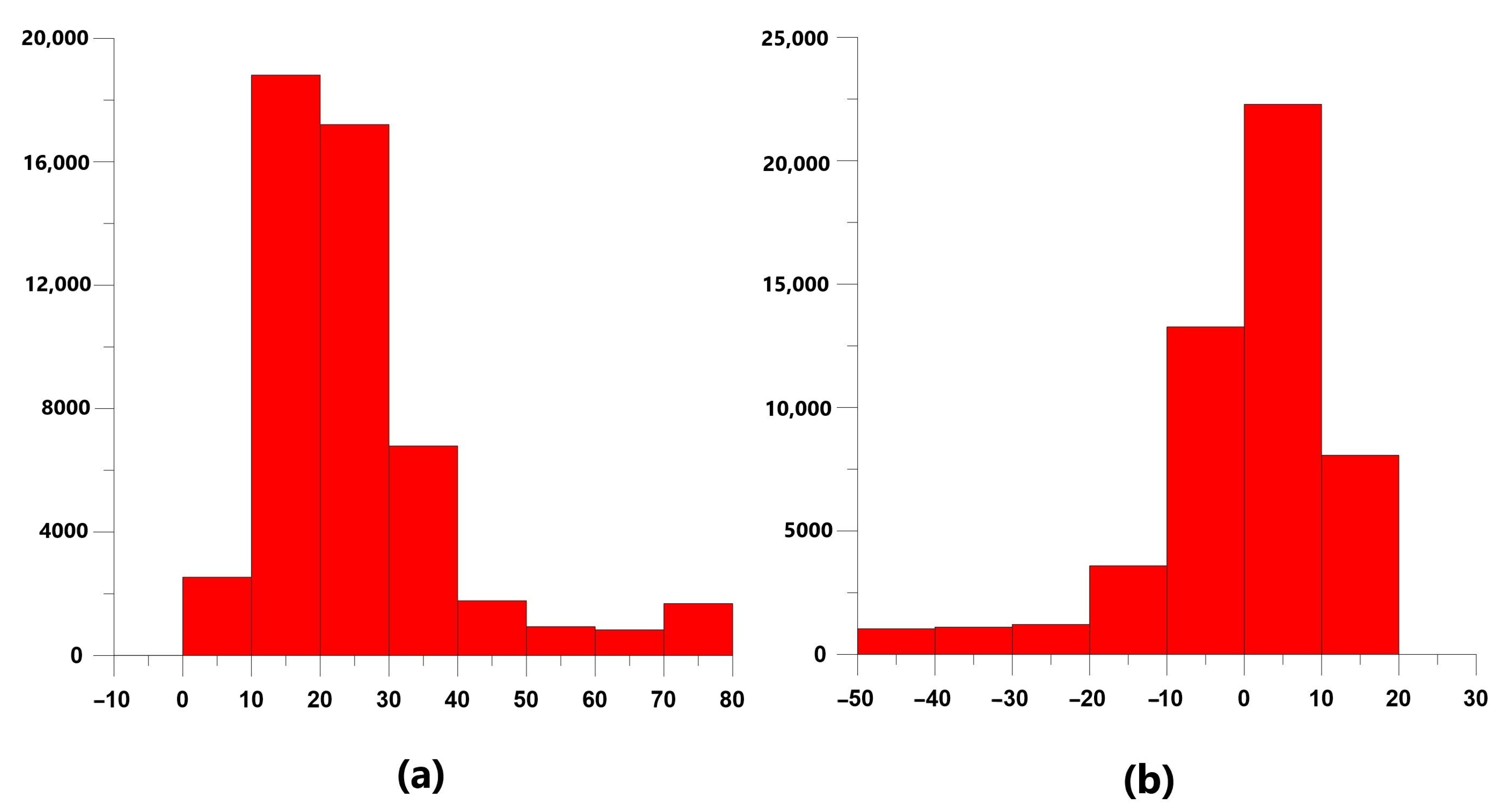
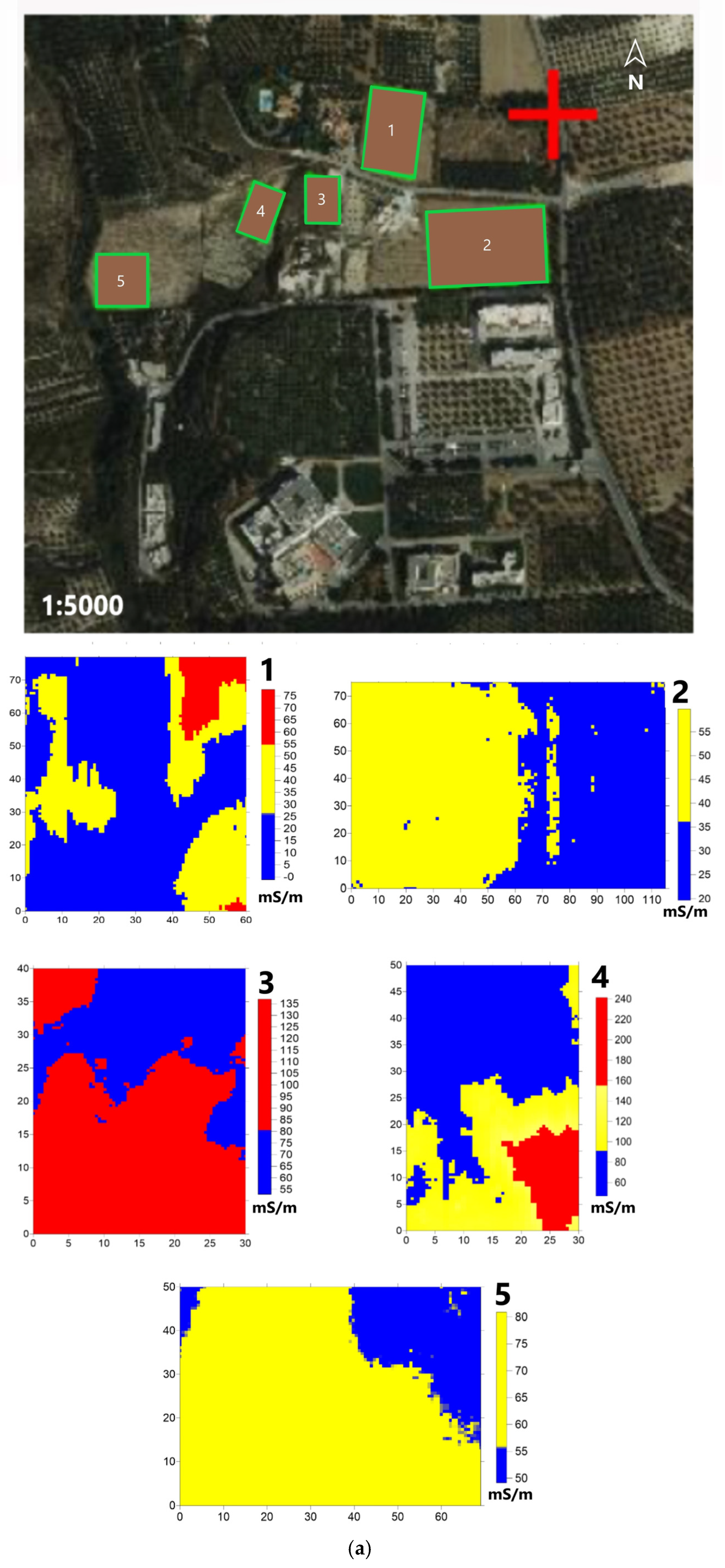
It is well known that mapping soil variability at plot level is a crucial step for the strategic management of agricultural fields to make farms more economically and ecologically sustainable and to protect the environment, especially near streams. Figure 8 presents the simple ratio (SR) vegetation index for the Gazanos Stream (area II). The riparian vegetation and the olive trees next to the stream of Gazanos present SR values higher than 15, while the soil presents values lower than 15. The SR index clearly facilitates the accurate mapping of vegetation and the differentiation from soil. Mapping, using GEM-2, was also carried out on agricultural parcels of area II in the wet period of 2022–2023. This area is covered by Pliocene sediments of the Finikia formation (Pl.m, Figure 1d). Figure 9 shows examples of intra-parcel soil zones for five parcels in area II defined according to two soil properties, namely, apparent electrical conductivity and magnetic susceptibility. For example, the apparent conductivity of the soil in parcel 1 ranges from 0 to 80 mS/m (Figure 9a), while the magnetic susceptibility of the soil ranges from −42 to 20 (10−5 S.I.) (Figure 9b), and the three soil zones were defined based on the histogram in Figure A1a,b (Appendix A). Similarly, two or three intra-parcel zones are also indicated in the rest four parcels (Figure 9a,b). Considering the distribution of apparent electrical conductivity and magnetic susceptibility in all five parcels mapped with GEM-2, we strongly believe that intra-parcel variability should be further investigated by conducting soil analyses.
5. Discussion
Water and soil are among the most important components for life and prosperity on our planet. However, the many competing pressures on the ecosystem services of water and soil are increasingly unsustainable, and climate change is exacerbating these pressures [60]. All over the world, environmental policy suffers from a lack of data to make targeted and efficient decisions. The need for highly accurate and detailed information is becoming increasingly urgent as the consequences of the climate crisis are now visible all over the planet. Earth observation based on satellite and aerial imagery (Figure 7 and Figure 8), supported by ground-based techniques (Figure 1, Figure 4, Figure 5, Figure 6 and Figure 9 and Table 1), is a unique source of data on natural resources and ecosystems to mitigate environmental hazards and ensure sustainable development [61,62,63,64,65,66]. As an example, we refer to Figure 7 of this paper, in which the IMD (%) corresponding to the percentage and change in soil sealing, is combined with the distribution of soil magnetic susceptibility in the lower part of the Karteros Stream, which is affected by agricultural and tourism activities as well as urbanisation. The part of the Karteros Stream marked by a red ellipse in Figure 7a is surrounded by branches of the transport network and has a (not so dense) urban structure that contributes to an IMD of more than 41%. Moreover, this part of the stream presents the relatively highest values (greater than 30 S.I. units) of χLF magnetic susceptibility (Figure 5 and Figure 7b). In addition, the morphology in this part of the Karteros Stream is mostly related with the north, northeast, and east aspects since the relief is smooth with slopes ranging between 0° and 20° (Figure 4). IMD (Figure 7a) also agrees with the prevailing aspects (Figure 4) in this part of the Karteros Stream.
Looking at the values of the real SIP conductivity of the Karteros water samples (Figure 6a), which range between 0.85 mS/cm and 1.2 mS/cm and are not far from the real conductivity of tap water (0.7 mS/cm), the water of the Karteros stream is not hard. The imaginary SIP conductivity of the Karteros water samples shows small fluctuations in the frequency range 0–1000 Hz (Figure 6b), indicating weak polarisation effects [51,53,54]. However, this part of the Karteros stream probably needs more attention in the sense that more specialised analyses of the stream water and soils around this part of the stream should be carried out in the future [23,25]. Specialised analyses of water quality could include physicochemical parameters (pH, electrical conductivity, salinity, chloride, and total hardness), nutrients (ammonium, phosphate, nitrate, and silicate) and photosynthetic pigments (chlorophyll-a, chlorophyll-b, and chlorophyll-c), while soil analyses could focus on geochemical analyses of metal concentrations (K, Ca, Ti, Mn, Fe, Ni, Cu, Zn, Pb, and others).
The presence of soil structures has not been explicitly considered in climate and Earth system models, partly due to incomplete methodological means to characterise them at relevant scales and parameterise them in spatially extended models [67]. Over the last two decades, efforts have been made to develop and standardise the use of geophysics for mapping soil properties (e.g., porosity, density, and clay content) and state variables (e.g., water content and salinity) [68,69,70]. In this work, the intra-parcel variability within plots next to the Gazanos Stream is investigated using electromagnetic methods (Figure 9a,b), and two or three soil zones are defined in each plot based on the spatial distribution of apparent conductivity and magnetic susceptibility. This soil zonation could be extremely helpful in the future agricultural management of the plots by reducing cultivation costs, increasing the quality and quantity of yields, and finally protecting the riparian environment of the Gazanos stream through the rational use of water, pesticides, and fertilisers. This is especially recommended for agricultural watersheds, as agricultural activities can greatly affect the well-being and health of aquatic systems. Streams are closely connected to their surrounding landscapes and reflect their watersheds, which, if impacted by agricultural practises, can lead to hydrological changes and/or the degradation of all water bodies flowing in the area. Finally, the Earth observation techniques can strongly support ecosystem services that are important for human life and well-being. Urban and suburban river and stream ecosystems provide important ecosystem services to their inhabitants and promote urban sustainability [71,72,73,74].
6. Conclusions
In this work, ground-based techniques from the related fields of digital topography, geology, and geophysics (spectral induced polarisation, apparent electrical conductivity, and magnetic susceptibility) are used together with remote sensing to provide (a) rapid, non-destructive, and cost-effective monitoring of urban and suburban aquatic bodies and the agricultural or urban land surrounding them, and (b) identify sites that are likely to be under environmental pressure and require further specialised water and soil analysis to confirm their possible contamination. We conclude with the following points:
- -
- Specialised topographic analyses have always been part of environmental and agricultural studies, as topography is one of the most important factors affecting the aquatic environment and agriculture.
- -
- The combination of spectral induced polarisation (real and imaginary components) and magnetic susceptibility using remote sensing seems ideal for rapid and cost-effective environmental monitoring.
- -
- Agricultural land west of Heraklion is dominated by intra-parcel soil variability. It is strongly recommended that intra-parcel soil variability be considered prior to any agricultural activity to support the rational use of inputs (water, pesticides, and fertilisers) and further protect the aquatic environment.
- -
- Topographic attributes such as slope and aspect, imperviousness density, vegetation indices, soil apparent electrical conductivity, soil magnetic susceptibility, and the spectral induced polarisation response of water (real and imaginary components, phase) are robust indicators for a rapid and cost-effective environmental investigation of rural and suburban areas bordering streams before conducting specific analyses.
Recommendations for the future include (a) the development of a standardised environmental protocol for monitoring the aquatic environment and agricultural activities in Crete and (b) the monitoring the temporal variability for selected water and soil indicators.
Author Contributions
Conceptualisation, D.C. and E.K.; methodology, E.K., D.C., S.K. and M.K.; software, E.K., D.C., S.K. and M.K.; validation, E.K., D.C., S.K. and M.K.; formal analysis, D.C. and E.K.; investigation, E.K., D.C., S.K. and M.K.; resources, D.C. and E.K.; data curation, E.K., D.C., S.K. and M.K.; writing—original draft preparation, D.C., E.K., S.K. and M.K.; writing—review and editing, D.C., E.K., S.K. and M.K.; visualisation, E.K., D.C., S.K. and M.K.; supervision, E.K.; project administration, E.K; funding acquisition, E.K. All authors have read and agreed to the published version of the manuscript.
Funding
Part of this work was conducted in the context of Project 101086521-OneAquaHealth-HORIZON-CL6-2022-GOVERNANCE-01 and the rest was supported by internal funding in the context of Ph.D. Studies and Diploma Dissertations.
Data Availability Statement
The datasets of the current study are available from the corresponding author on reasonable request.
Acknowledgments
The authors are grateful to the editor, assistant editor, and the anonymous reviewers for their critical review and constructive comments.
Conflicts of Interest
The authors declare no conflict of interest.
Appendix A
Figure A1.
Example of how histograms were used to determine the spatial variability of the agricultural parcel 1 shown in Figure 7. They present the distribution of (a) conductivity and (b) magnetic susceptibility.
Figure A1.
Example of how histograms were used to determine the spatial variability of the agricultural parcel 1 shown in Figure 7. They present the distribution of (a) conductivity and (b) magnetic susceptibility.
References
- Brazeau, S.; Ogden, N.H. Earth Observation, Public Health and One Health: Activities, Challenges and Opportunities; CABI: Wallingford, UK, 2022; pp. 1–106. [Google Scholar] [CrossRef]
- Neiderud, C.-J. How urbanization affects the epidemiology of emerging infectious diseases. Infect. Ecol. Epidemiol. 2015, 5, 1. [Google Scholar] [CrossRef]
- Jones, B.A.; Grace, D.; Kock, R.; Alonso, S.; Rushton, J.; Said, M.Y.; McKeever, D.; Mutua, F.; Young, J.; McDermott, J.; et al. Zoonosis emergence linked to agricultural intensification and environmental change. Proc. Natl. Acad. Sci. USA 2013, 110, 8399–8404. [Google Scholar] [CrossRef]
- Keesing, F.; Belden, L.K.; Daszak, P. Impacts of biodiversity on the emergence and transmission of infectious diseases. Nature 2010, 468, 647–652. [Google Scholar] [CrossRef]
- Ostfeld, R.S.; Keesing, F. Effects of host diversity on infectious disease. Annu. Rev. Ecol. Evol. Syst. 2012, 43, 157–182. [Google Scholar] [CrossRef]
- Altizer, S.; Ostfeld, R.S.; Johnson, P.T.; Kutz, S.; Harvell, C.D. Climate change and infectious diseases: From evidence to a predictive framework. Science 2013, 341, 514–519. [Google Scholar] [CrossRef] [PubMed]
- Oakley, A.L.; Collins, J.; Everson, L.; Heller, D.; Howerton, J.; Vincent, R. Riparian zones and freshwater wetlands. In Management of Wildlife and Fish Habitats in Forest of Western Oregon and Washington; US Department of Agriculture, Forest Service: Pacific Northwest Region, OR, USA, 1985; pp. 57–80. [Google Scholar]
- Odum, E.P. Ecological Importance of the Riparian Zone; General Technical Report WO-US; Department of Agriculture, Forest Service: Washington, DC, USA, 1979.
- Doufexi, M.; Gamvroula, D.E.; Alexakis, D.E. Elements’ Content in Stream Sediment and Wildfire Ash of Suburban Areas in West Attica (Greece). Water 2022, 14, 310. [Google Scholar] [CrossRef]
- Tha, T.; Piman, T.; Bhatpuria, D.; Ruangrassamee, P. Assessment of Riverbank Erosion Hotspots along the Mekong River in Cambodia Using Remote Sensing and Hazard Exposure Mapping. Water 2022, 14, 1981. [Google Scholar] [CrossRef]
- Wohl, E.; Castro, J.; Cluer, B.; Merritts, D.; Powers, P.; Staab, B.; Thorne, C. Rediscovering, Reevaluating, and Restoring Lost River-Wetland Corridors. Front. Earth Sci. 2021, 9, 511. [Google Scholar] [CrossRef]
- Barnett, Z.C.; Adams, S.B. Review of Dam Effects on Native and Invasive Crayfishes Illustrates Complex Choices for Conservation Planning. Front. Ecol. Evol. 2021, 8, 621723. [Google Scholar] [CrossRef]
- Wymore, A.S.; Ward, A.S.; Wohl, E.; Harvey, J.W. Viewing river corridors through the lens of critical zone science. Front. Water 2023, 5, 1147561. [Google Scholar] [CrossRef]
- Harvey, J.; Gooseff, M. River corridor science: Hydrologic exchange and ecological consequences from bedforms to basins. Water Resour. Res. 2015, 50, 6893–6922. [Google Scholar] [CrossRef]
- Van der Werf, H.M.G. Assessing the impact of pesticides on the environment. Agric. Ecosyst. Environ. 1996, 60, 81–96. [Google Scholar] [CrossRef]
- Reichenberger, S.; Bach, M.; Skitschak, A.; Frede, H.G. Mitigation strategies to reduce pesticide inputs into the ground- and surface water and their effectiveness. A review. Sci. Total Environ. 2007, 384, 1–35. [Google Scholar] [CrossRef] [PubMed]
- Directive 2009/128/EC of the European Parliament and of the Council of 21 October 2009 establishing a framework for Community action to achieve the sustainable use of pesticides. Off. J. Eur. Union 2009, L 309, 71–86.
- Navarro, S.; Vela, N.; Navarro, G. An overview on the environmental behaviour of pesticide residues in soils. Span. J. Agric. Res. 2007, 5, 357–375. [Google Scholar] [CrossRef]
- Kordel, W.; Klein, M. Prediction of leaching and groundwater contamination by pesticides. Pure Appl. Chem. 2006, 78, 1081–1090. [Google Scholar] [CrossRef]
- Tank, J.L.; Speir, S.L.; Sethna, L.R.; Royer, T.V. The Case for Studying Highly Modified Agricultural Streams: Farming for Biogeochemical Insights. Limnol. Oceanogr. Bull. 2021, 30, 41–47. [Google Scholar] [CrossRef]
- Blann, K.L.; Anderson, J.L.; Sands, G.R.; Vondracek, B. Effects of agricultural drainage on aquatic ecosystems: A review. Crit. Rev. Environ. Sci. Technol. 2009, 39, 909–1001. [Google Scholar] [CrossRef]
- Diaz, R.J.; Rosenberg, R. Spreading dead zones and consequences for marine ecosystems. Science 2008, 321, 926–929. [Google Scholar] [CrossRef]
- Sarris, A.; Kokinou, E.; Aidona, E.; Kallithrakas-Kontos, N.; Koulouridakis, P.; Kakoulaki, G.; Droulia, K.; Damianovits, O. Environmental study for pollution in the area of the Megalopoli power plant (Peloponnesus, Greece). Environ. Geol. 2009, 58, 1769–1783. [Google Scholar] [CrossRef]
- Kokinou, E.; Belonaki, C.; Sakadakis, D.; Sakadaki, K. Environmental monitoring of soil pollution in urban areas (a case study from Heraklion city, Central Crete, Greece). Bull. Geol. Soc. Greece 2013, 47, 963–971. [Google Scholar] [CrossRef]
- Kokinou, E.; Zacharioudaki, D.; Kokolakis, S.; Kotti, M.; Chatzidavid, D.; Karagiannidou, M.; Fanouraki, E.; Kontaxakis, E. Spatiotemporal environmental monitoring of the karst-related Almyros Wetland (Heraklion, Crete, Greece, Eastern Mediterranean). Environ. Monit. Assess. 2023, 195, 955. [Google Scholar] [CrossRef] [PubMed]
- Briassoulis, H. Crete: Endowed by Nature, Privileged by Geography, Threatened by Tourism? J. Sustain. Tour. 2003, 11, 97–115. [Google Scholar] [CrossRef]
- Barboutis, C.; Navarrete, E.; Karris, G.; Xirouchakis, S.; Fransson, T.; Bounas, A. Arriving depleted after crossing of the Mediterranean: Obligatory stopover patterns underline the importance of Mediterranean islands for migrating birds. Anim. Migr. 2022, 9, 14–23. [Google Scholar] [CrossRef]
- Vidakis, Μ.; Meulenkamp, J.E.; Koutsouveli, A.; Ioakim, C.; Papazeti, E.; Skourtsi-Koronaiou, V. Geological Map of Greece in 1:50,000 scale—Heraklion Sheet. IGME Athens 1996. [Google Scholar]
- Roberts, G.G.; White, N.J.; Shaw, B. An uplift history of Crete, Greece, from inverse modeling of longitudinal river profiles. Geomorphology 2013, 198, 177–188. [Google Scholar] [CrossRef]
- Strahler, A.N. Quantitative analysis of watershed geomorphology. Trans. Am. Geophys. Union 1957, 38, 913–920. [Google Scholar]
- Rackham, O.; Moody, J. The Making of the Cretan Landscape; Manchester University Press: Manchester, UK, 1996. [Google Scholar]
- Vogiatzakis, I.; Mannion, A.M.; Pungetti, G. Introduction to the Mediterranean Island Landscapes. In Mediterranean Island Landscapes; Landscape Series; Vogiatzakis, I., Pungetti, G., Mannion, A.M., Eds.; Springer: Dordrecht, The Netherlands, 2008; Volume 9. [Google Scholar] [CrossRef]
- Kokinou, E.; Skilodimou, H.D.; Bathrellos, G.D.; Antonarakou, A.; Kamberis, E. Morphotectonic analysis, structural evolution/pattern of a contractional ridge: Giouchtas Mt., Central Crete, Greece. J. Earth Syst. Sci. 2015, 124, 587–602. [Google Scholar]
- Kokinou, E. Magnetic properties of soils in a designated Natura area (GR4310010, Giouchtas Mountain). SEG Interpret. 2015, 3, SAB33–SAB42. [Google Scholar] [CrossRef]
- Ministry of Environment & Energy—Department of Energy. Preparation of the 1st Revision of the River Basin Management Plan of the Republic of Crete (EL 13), Intermediate Phase: 2. Deliverable 18; Strategic Environmental Impact Assessment (SEA): Athens, Greece, 2017. [Google Scholar]
- Panagiotakis, C.; Kokinou, E. Linear Pattern Detection of Geological Faults via a Topology and Shape Optimization Method. IEEE J. Sel. Top. Appl. Earth Obs. Remote Sens. 2015, 8, 3–11. [Google Scholar] [CrossRef]
- Toulia, E.; Kokinou, E.; Panagiotakis, C. The contribution of pattern recognition techniques in geomorphology and geology: The case study of Tinos Island (Cyclades, Aegean, Greece). Eur. J. Remote Sens. 2018, 51, 88–99. [Google Scholar] [CrossRef]
- Kokinou, E.; Panagiotakis, C. Structural pattern recognition applied on bathymetric data from the Eratosthenes Seamount (Eastern Mediterranean, Levantine Basin). Geo-Mar. Lett. 2018, 38, 527–540. [Google Scholar] [CrossRef]
- Kokinou, E.; Panagiotakis, C. Automatic Pattern Recognition of Tectonic Lineaments in Seafloor Morphology to Contribute in the Structural Analysis of Potentially Hydrocarbon-Rich Areas. Remote Sens. 2020, 12, 1538. Available online: https://www.mdpi.com/2072-4292/12/10/1538 (accessed on 15 April 2023). [CrossRef]
- Kokinou, E. Automatic pattern recognition and GPS/GNSS technology in marine digital terrain model. In GPS and GNSS Technology in Geosciences; Petropoulos, G., Srivastava, P., Eds.; Elsevier: Amsterdam, The Netherlands, 2021; pp. 241–254. Available online: https://www.sciencedirect.com/science/article/pii/B9780128186176000196 (accessed on 15 April 2023).
- Kasapaki, A. Spatial Distribution of the Magnetic Susceptibility along the Drainage Network of Karteros in Heraklion Crete. Bachelor’s Thesis, Hellenic Mediterranean University, Chania, Greece, 2009. Available online: http://hdl.handle.net/11713/2574 (accessed on 29 April 2023).
- Scholger, R. Heavy metal pollution monitoring by magnetic susceptibility measurements applied to sediments of the river Mur (Styria, Austria). Eur. J. Envirn. Eng. Geophys. 1998, 3, 25–37. [Google Scholar]
- Bityukova, L.; Scholger, R.; Birke, M. Magnetic susceptibility as indicator of environmental pollution of soils in Tallinn (Estonia). Phys. Chem. Earth 1999, 24, 829–835. [Google Scholar] [CrossRef]
- Petrovsky, E.; Kapička, A.; Jordanova, N.; Borůvka, L. Magnetic properties of alluvial soils contaminated with lead, zinc and cadmium. J. Appl. Geophys. 2001, 48, 127–136. [Google Scholar] [CrossRef]
- Boyko, T.; Scholger, R.; Stanjek, H.; MAGPROX Team. Topsoil magnetic susceptibility mapping as a tool for pollution monitoring: Repeatability of in situ measurements. J. Appl. Geophys. 2004, 55, 249–259. [Google Scholar] [CrossRef]
- Thompson, T.; Oldfield, F. (Eds.) Environmental Magnetism; Allen and Unwin: London, UK, 1986. [Google Scholar]
- Kokinou, E.; Papadopoulos, I.; Vallianatos, F. A geophysical survey on marls of Heraklion city in Crete Island (Southern Hellenic Arc, Greece). In Proceedings of the 2nd International Conference on Engineering Mechanics, Structures, Engineering Geology (EMESEG ’09), Rhodes Island, Greece, 22–24 July 2009; pp. 202–207, ISBN 978-960-474-101-4. [Google Scholar]
- Savvaidis, A.; Margaris, B.; Theodoulidis, N.; Lekidis, V.; Karakostas, C.; Loupasakis, C.; Rozos, D.; Soupios, P.; Mangriotis, M.-D.; Dikmen, U.; et al. Geo-Characterization at selected accelerometric stations in Crete (Greece) and comparison of earthquake data recordings with EC8 elastic spectra. Cent. Eur. J. Geosci. 2014, 6, 88–103. [Google Scholar] [CrossRef]
- Atekwana, E.A.; Slater, L.D. Biogeophysics: A new frontier in Earth science research. Rev. Geophys. 2009, 47, RG4004. [Google Scholar] [CrossRef]
- Revil, A.; Karaoulis, M.; Johnson, T.; Kemna, A. Review: Some low-frequency electrical methods for subsurface characterization and monitoring in hydrogeology. Hydrogeol. J. 2012, 20, 617–658. [Google Scholar] [CrossRef]
- Kemna, A.; Binley, A.; Cassiani, G.; Niederleithinger, E.; Revil, A.; Slater, L.; Williams, K.H.; Orozco, A.F.; Haegel, F.H.; Hördt, A.; et al. An overview of the spectral induced polarization method for near-surface applications. Near Surf. Geophys. 2012, 10, 453–468. [Google Scholar] [CrossRef]
- Kirmizakis, P.; Kalderis, D.; Ntarlagiannis, D.; Soupios, P. Preliminary assessment on the application of biochar and spectral induced polarization for wastewater treatment. Near Surf. Geophys. 2020, 18, 109–122. [Google Scholar] [CrossRef]
- Slater, L.D.; Lesmes, D. IP interpretation in environmental investigations. Geophysics 2002, 67, 77–88. [Google Scholar] [CrossRef]
- Binley, A.; Kemna, A. DC Resistivity and Induced Polarization Methods. Hydrogeophysics 2005, 50, 129–156. [Google Scholar]
- Kumhálová, J.; Kumhála, F.; Kroulík, M. The impact of topography on soil properties and yield and the effects of weather conditions. Precis. Agric. 2011, 12, 813–830. [Google Scholar] [CrossRef]
- Bakhsh, A.; Colvin, T.S.; Jaynes, D.B.; Kanwar, R.S.; Tim, U.S. Using soil attributes and GIS for interpretation of spatial variability in yield. Trans. ASABE 2000, 43, 819–828. [Google Scholar] [CrossRef]
- Kravchenko, A.N.; Bullock, D.G. Correlation of corn and soybean grain yield with topography and soil properties. J. Agron. 2000, 92, 75–83. [Google Scholar] [CrossRef]
- Kravchenko, A.N.; Bullock, D.G. Spatial variability of soybean quality data as a function of field topography: I, spatial data analysis. Crop. Sci. 2002, 42, 804–815. [Google Scholar] [CrossRef]
- Jenson, S.K.; Domingue, J.O. Extracting topographic structure from digital elevation data for geographic information system analysis. Photogramm. Eng. Remote Sens. 1988, 54, 1593–1600. Available online: https://pubs.usgs.gov/publication/70142175 (accessed on 25 May 2023).
- Agnoli, L.; Urquhart, E.; Georgantzis, N.; Schaeffer, B.; Simmons, R.; Hoque, B.; Neely, M.B.; Neil, C.; Oliver, J.; Tyler, A. Perspectives on user engagement of satellite Earth observation for water quality management. Technol. Forecast. Soc. Chang. 2023, 189, 122357. [Google Scholar] [CrossRef]
- Ferreira, B.; Iten, M.; Silva, R.G. Monitoring sustainable development by means of Earth observation data and machine learning: A review. Environ. Sci Eur. 2020, 32, 120. [Google Scholar] [CrossRef]
- Pasher, J.; Smith, P.A.; Forbes, M.R.; Duffe, J. Terrestrial ecosystem monitoring in Canada and the greater role for integrated Earth observation. Environ. Rev. 2014, 22, 179–187. [Google Scholar] [CrossRef]
- Ramirez-Reyes, C.; Brauman, K.A.; Chaplin-Kramer, R.; Galford, G.L.; Adamo, S.B.; Anderson, C.B.; Anderson, C.; Allington, G.R.H.; Bagstad, K.J.; Coe, M.T.; et al. Reimagining the potential of Earth observations for ecosystem service assessments. Sci. Total Environ. 2019, 665, 1053–1063. [Google Scholar] [CrossRef] [PubMed]
- Crocetti, L.; Forkel, M.; Fischer, M.; Jurečka, F.; Grlj, A.; Salentinig, A.; Trnka, M.; Anderson, M.; Ng, W.-T.; Kokalj, Ž.; et al. Earth observation for agricultural drought monitoring in the Pannonian Basin (Southeastern Europe): Current state and future directions. Reg. Environ. Chang. 2020, 20, 123. [Google Scholar] [CrossRef]
- Lawford, R.; Strauch, A.; Toll, D.; Fekete, B.; Cripe, D. Earth observations for global water security. Curr. Opin. Environ. Sustain. 2013, 5, 633–643. [Google Scholar] [CrossRef]
- Uereyen, S.; Kuenzer, C. A review of Earth observation-based analyses for major river basins. Remote Sens. 2019, 11, 2951. [Google Scholar] [CrossRef]
- Romero-Ruiz, A.; Linde, N.; Keller, T.; Or, D. A Review of Geophysical Methods for Soil Structure Characterization. Rev. Geophys. 2018, 56, 672–697. [Google Scholar] [CrossRef]
- Samouelian, A.; Cousin, I.; Tabbagh, A.; Bruand, A.; Richard, G. Electrical resistivity survey in soil science: A review. Soil Tillage Res. 2005, 83, 173–193. [Google Scholar] [CrossRef]
- Allred, B.J.; Daniels, J.J.; Ehsani, M.R. Handbook of Agricultural Geophysics; CRC Press: Boca Raton, FL, USA, 2008. [Google Scholar]
- Kritikakis, G.; Kokinou, E.; Economou, N.; Andronikidis, N.; Brintakis, J.; Daliakopoulos, I.N.; Kourgialas, N.; Pavlaki, A.; Fasarakis, G.; Markakis, N.; et al. Estimating Soil Clay Content Using an Agrogeophysical and Agrogeological Approach: A Case Study in Chania Plain, Greece. Water 2022, 14, 2625. [Google Scholar] [CrossRef]
- Grimm, N.B.; Faeth, S.H.; Golubiewski, N.E.; Redman, C.L.; Wu, J.; Bai, X.; Briggs, J.M. Global change and the ecology of cities. Science 2008, 319, 756–760. [Google Scholar] [CrossRef]
- Haase, D. Reflections about blue ecosystem services in cities. Sustain. Water Qual. Ecol. 2015, 5, 77–83. [Google Scholar] [CrossRef]
- Elmqvist, T.; Setälä, H.; Handel, S.N.; van der Ploegn, S.; Aronson, J.; Blignaut, J.N.; Gómez-Baggethun, E.; Nowak, D.J.; Kronenberg, J.; de Groot, R. Benefits of restoring ecosystem services in urban areas. Curr. Opin. Environ. Sustain. 2015, 14, 101–108. [Google Scholar] [CrossRef]
- Calapez, A.R.; Serra, S.R.Q.; Mortágua, A.; Almeida, S.F.P.; João Feio, M. Unveiling relationships between ecosystem services and aquatic communities in urban streams. Ecol. Indic. 2023, 153, 110433. [Google Scholar] [CrossRef]
Figure 2.
The natural environment of this study: (a–d) correspond to area I, while (e,f) correspond to area II (Figure 1b).
Figure 2.
The natural environment of this study: (a–d) correspond to area I, while (e,f) correspond to area II (Figure 1b).
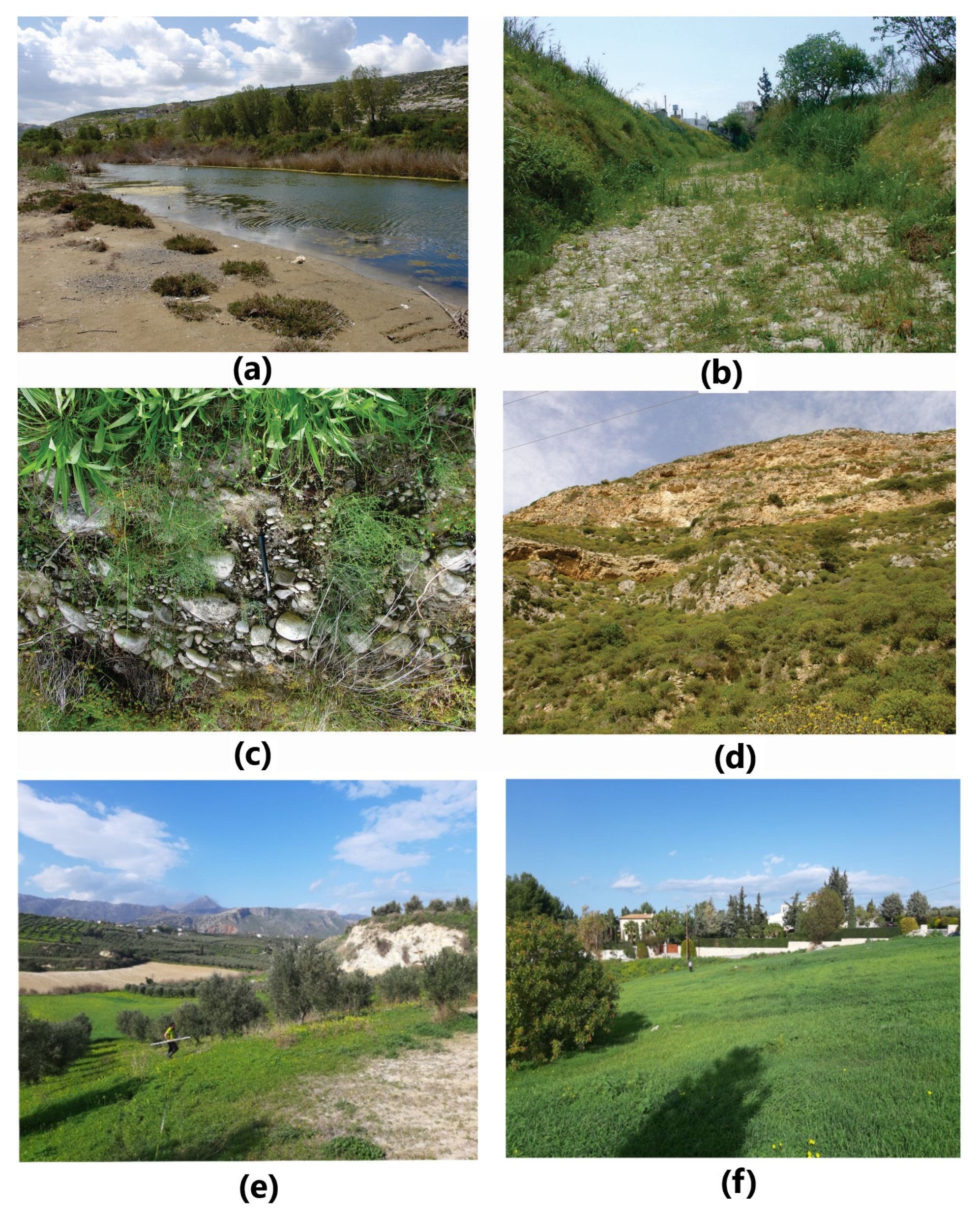
Figure 3.
Flow chart of the methodological steps.
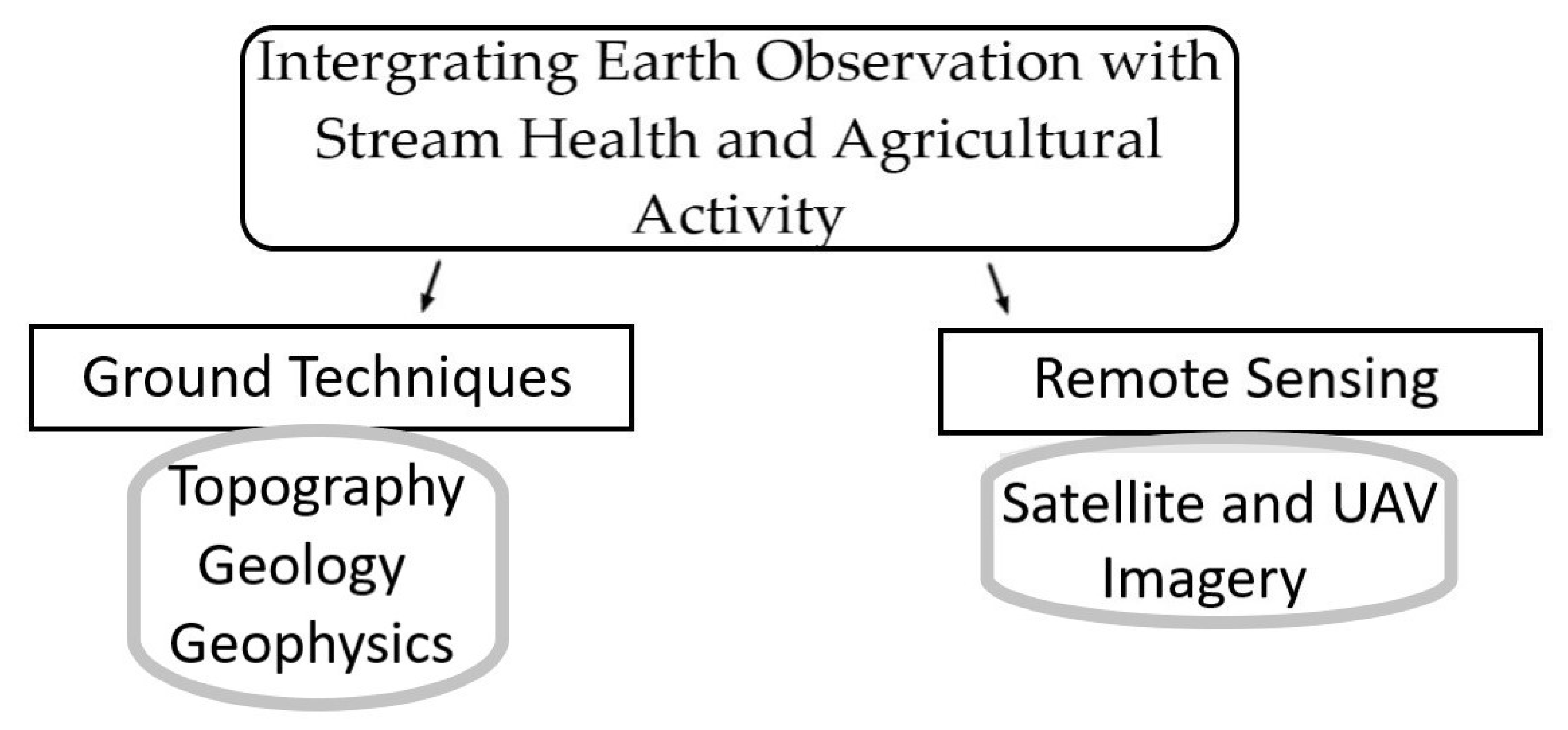
Figure 4.
Topographic analyses for area I (Figure 1b) on data from topographic maps of scale of 1:5000, published by the Hellenic Army Geographical Service (H.A.G.S.). The upper left image shows the elevation (m), the upper right image shows the slopes (°), the lower left image presents the aspects (°), and the lower right image corresponds to the automatic detections based on [36].
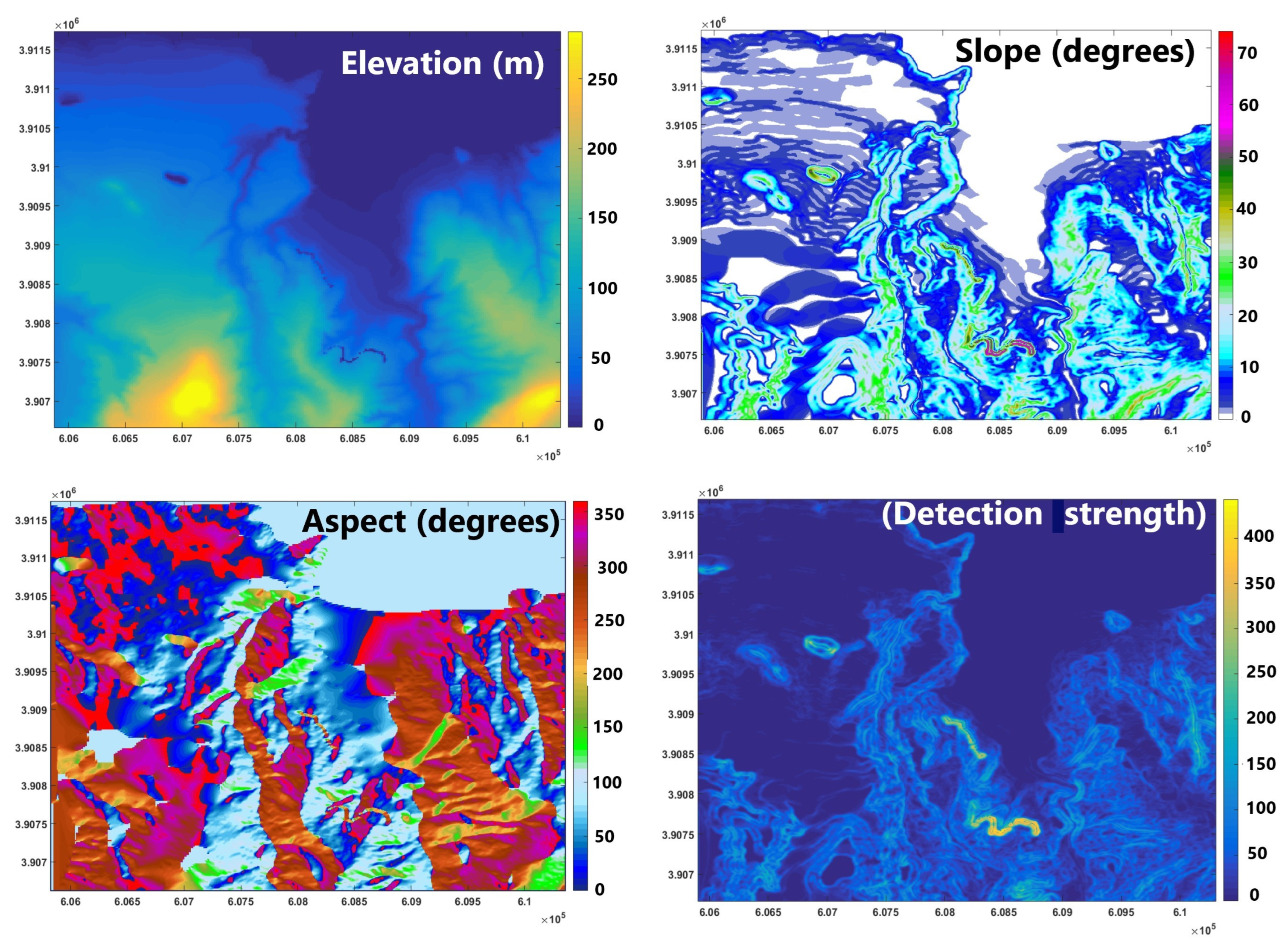
Figure 5.
Distribution of low-field magnetic susceptibility (LFS) for area I (Figure 1c).
Figure 5.
Distribution of low-field magnetic susceptibility (LFS) for area I (Figure 1c).

Figure 6.
SIP response of the six (6) water samples from Karteros Canyon (area I, Figure 1b), tap water analysis included for comparison; (a,b) real and imaginary conductivity versus frequency; (c) frequency versus phase.
Figure 6.
SIP response of the six (6) water samples from Karteros Canyon (area I, Figure 1b), tap water analysis included for comparison; (a,b) real and imaginary conductivity versus frequency; (c) frequency versus phase.
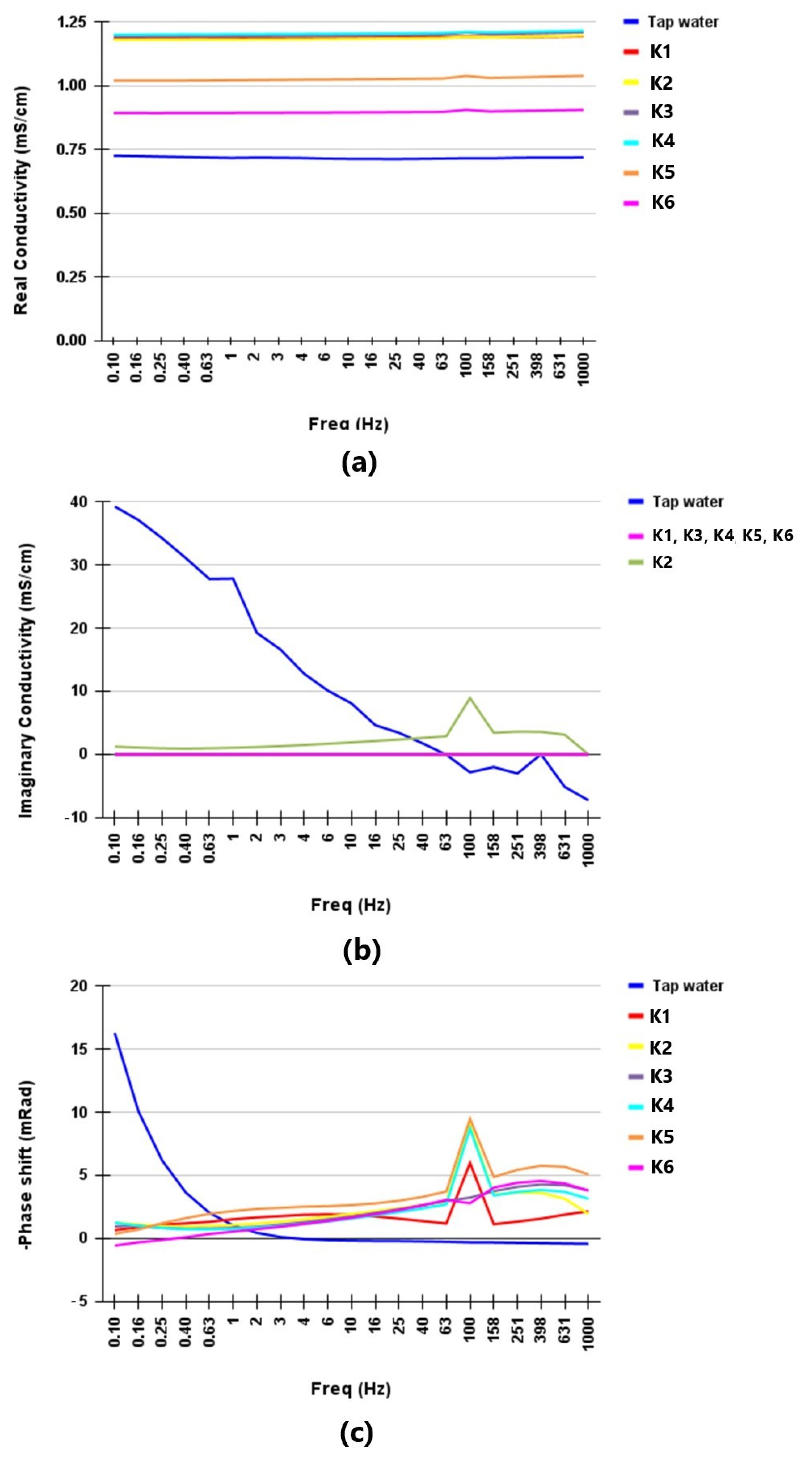
Figure 7.
Comparison of (a) imperviousness density (IMD %) and (b) low-field magnetic susceptibility (LFS) in part of Karteros Stream (area I). Red ellipse indicates the site of Karteros Stream (area I) showing both relatively higher values of IMD and LFS. The traffic network is indicated by the orange line, the hydrographic network, and the coastline with blue line while the geological faults are indicated with the black line.

Figure 8.
The simple ratio (SR) index in Gazanos Stream, area II (UAV flight, DJI Mavik 3M, 22 August 2023).
Figure 8.
The simple ratio (SR) index in Gazanos Stream, area II (UAV flight, DJI Mavik 3M, 22 August 2023).

Figure 9.
Distribution of (a) the soil conductivity and (b) magnetic susceptibility for the agricultural parcels shown in the upper part of figure (a) (National Cadastre, https://www.ktimatologio.gr/en (accessed on 15 June 2023)) in area II (Figure 1b).
Figure 9.
Distribution of (a) the soil conductivity and (b) magnetic susceptibility for the agricultural parcels shown in the upper part of figure (a) (National Cadastre, https://www.ktimatologio.gr/en (accessed on 15 June 2023)) in area II (Figure 1b).


Table 1.
Characterisation of the stratigraphy in area I (Figure 1c).
Table 1.
Characterisation of the stratigraphy in area I (Figure 1c).
| Formation | Thickness (m) | Seismic Velocity (km/s) | Resistivity (Ohm.m) | Low-Frequency (Flow = 0.43 KHz) Background Magnetic Susceptibility (SI Units) |
|---|---|---|---|---|
| Holocene—Fluvial and closed basin deposits (al) | Up to 25 | 0.7–1 | 15–30 | ~16.5 |
| Holocene—Marine terraces and coastal sands (Pt.m) | 2–4 | 0.2–0.3 | >20 | ~15.2 |
| Lower–Middle Pliocene—Finikia formation (Pl.m) | >150 | ~1.4 | 20–150 | ~18 |
| Upper Miocene—Ag. Varvara formation (M.k, M.m) | ~280 | 1.4–1.8 | 250–500 | Not measured |
| Upper Triassic–Upper Jurassic Limestones (Ts-Js.Kd) | Up to 300 | 5.4–5.8 | 2000–2500 | Not measured |
Disclaimer/Publisher’s Note: The statements, opinions and data contained in all publications are solely those of the individual author(s) and contributor(s) and not of MDPI and/or the editor(s). MDPI and/or the editor(s) disclaim responsibility for any injury to people or property resulting from any ideas, methods, instructions or products referred to in the content. |
© 2023 by the authors. Licensee MDPI, Basel, Switzerland. This article is an open access article distributed under the terms and conditions of the Creative Commons Attribution (CC BY) license (https://creativecommons.org/licenses/by/4.0/).
Share and Cite
MDPI and ACS Style
Chatzidavid, D.; Kokinou, E.; Kokolakis, S.; Karagiannidou, M. Integrating Earth Observation with Stream Health and Agricultural Activity. Remote Sens. 2023, 15, 5485. https://doi.org/10.3390/rs15235485
AMA Style
Chatzidavid D, Kokinou E, Kokolakis S, Karagiannidou M. Integrating Earth Observation with Stream Health and Agricultural Activity. Remote Sensing. 2023; 15(23):5485. https://doi.org/10.3390/rs15235485
Chicago/Turabian StyleChatzidavid, David, Eleni Kokinou, Stratos Kokolakis, and Matina Karagiannidou. 2023. "Integrating Earth Observation with Stream Health and Agricultural Activity" Remote Sensing 15, no. 23: 5485. https://doi.org/10.3390/rs15235485
Note that from the first issue of 2016, this journal uses article numbers instead of page numbers. See further details here.