Article

Evaluating the Performance of Geographic Object-Based Image Analysis in Mapping Archaeological Landscapes Previously Occupied by Farming Communities: A Case of Shashi–Limpopo Confluence Area

by
Olaotse Lokwalo Thabeng
1,2,*,
Elhadi Adam
2 and
Stefania Merlo
3
1
Archaeology Unit, University of Botswana, 4775 Corner Notwane Rd, Gaborone Private Bag 00703, Botswana
2
School of Geography, Archaeology and Environmental Studies, University of the Witwatersrand, Johannesburg 2050, South Africa
3
McDonald Institute for Archaeological Research, Downing Street, Cambridge CB2 3ER, UK
*
Author to whom correspondence should be addressed.
Remote Sens. 2023, 15(23), 5491; https://doi.org/10.3390/rs15235491
Submission received: 6 July 2023 / Revised: 3 September 2023 / Accepted: 12 September 2023 / Published: 24 November 2023

Abstract

:
The use of pixel-based remote sensing techniques in archaeology is usually limited by spectral confusion between archaeological material and the surrounding environment because they rely on the spectral contrast between features. To deal with this problem, we investigated the possibility of using geographic object-based image analysis (GEOBIA) to predict archaeological and non-archaeological features. The chosen study area was previously occupied by farming communities and is characterised by natural soils (non-sites), vitrified dung, non-vitrified dung, and savannah woody vegetation. The study uses a three-stage GEOBIA that comprises (1) image object segmentation, (2) feature selection, and (3) object classification. The spectral mean of each band and the area extent of an object were selected as input variables for object classifications in support vector machines (SVM) and random forest (RF) classifiers. The results of this study have shown that GEOBIA approaches have the potential to map archaeological landscapes. The SVM and RF classifiers achieved high classification accuracies of 96.58% and 94.87%, respectively. Visual inspection of the classified images has demonstrated the importance of the aforementioned models in mapping archaeological and non-archaeological features because of their ability to manage the spectral confusion between non-sites and vitrified dung sites. In summary, the results have demonstrated that the GEOBIAs ability to incorporate spatial elements in the classification model ameliorates the chances of distinguishing materials with limited spectral differences.

Graphical Abstract

1. Introduction

Remote sensing has proved to be a vital instrument for the survey, documentation, and monitoring of archaeological sites [1,2]. It offers a relatively cheap, fast, systematic, and reproducible method of survey, which is capable of documenting and monitoring archaeological sites across huge and/or inaccessible locations within a short period [3,4,5]. The use of remote sensing in archaeology commonly exploits the spectral difference between archaeological features and their surrounding [6,7]. This is largely because past anthropogenic activities have a localised impact on the soil’s chemical and physical properties, therefore, making it different from its surroundings [8,9]. A key requirement in remote sensing image analysis is the decision concerning the basic unit of classification, which can either be an image pixel or an image object [10,11,12,13]. The image pixel is the smallest discrete area within a two-dimensional array of cells that forms an image. The image object is created by grouping spatially connected pixels with homogeneous properties using segmentation analysis [10,14,15].
Different pixel-based image classifiers have been tested in archaeological applications using imagery captured by hyperspectral and multispectral sensors [16,17,18,19,20]. Image enhancement techniques have been mainly employed to increase the prominence and identification of archaeological features in an image [19,21]. For example, the principal component analysis was used to enhance the spectral differences of cropmarks associated with archaeological sites in southern Scotland, therefore improving the visibility and identification of archaeological features in the landscape [16]. Bennett et al. [22] used normalised vegetation indices to identify archaeological sites in the grasslands of Salisbury Plain, Wiltshire. On the other hand, some researchers used unsupervised pixel-based classifiers to assess the possibility of spectrally separating archaeological features from their surroundings and identifying unknown classes [4,23,24,25]. Ciminale et al. [26] used the ISODATA unsupervised classifier to identify paleo-riverbeds which cut through the ditches of the Neolithic village of Schifata in Northern Italy. The main challenge of using unsupervised classifiers is that an analyst does not develop reference data classes that will be used in training the classification model [27]. As a result, the classifiers produce meaningless classes of data, which can be challenging to merge into meaningful classes [28]. Researchers [20,29,30] employed supervised pixel-based classifiers to predict areas of archaeological interest.
The pixel-based methods have produced high classification accuracies in detecting most of the archaeological sites. However, some limitations associated with the pixel-based methods in archaeological applications have been reported in recent studies [20,31]. Pixel-based classifiers cannot handle within-class spectral variability [32]. Above all, the major issue with the application of the aforementioned classification methods is that they assume the pixel as the spatial unit of analysis and depend solely on its spectral properties for classification [15]. This becomes problematic in archaeological sites and environments characterised by features with variance in material composition and spatial attributes but having similar spectral signatures [32,33]. For example, despite the difference in their spatial attributes, Thabeng et al. [20] found that there is no spectral difference between vitrified dung deposits and non-sites. The confusion between the two features might be because of their similar whitish colour or the washing down of dung deposits into the river by water erosion, which is rampant in the area. As a result, this calls for the classification process, which will incorporate spatial attributes of the aforementioned features, such as texture and size, in addition to spectral properties, to achieve accuracy improvement.
GEOBIA has been used to differentiate features with similar spectral characteristics and different spatial, textural, and contextual properties [15,33,34,35]. Research has also shown that GEOBIA is superior to pixel-based classifications, especially, in complex environments [33,36] and on images with limited spectral details [37]. For instance, Myint et al. [15] proved that GEOBIA outclassed pixel-based analysis when mapping the central part of the city of Phoenix in Arizona, which was characterised by spectrally similar feature classes. In their study, the object-based classifier outperformed the pixel-based maximum likelihood classifier by 22.8% as they achieved an overall accuracy of 90.40% and 67.60%, respectively. Furthermore, GEOBIA has been used for classification in numerous Land Cover Land Use (LULC) research, which include agriculture [10,38,39], urban landscapes [14,40,41,42], and vegetation mapping [43], where it achieved excellent results. Lately, GEOBIA has been used to delineate landforms for the prediction of archaeological sites [31,44] and detect looting activities [45]. Conversely, this method has not been tested in discriminating against surface archaeological deposits of vitrified dung, non-vitrified dung, and non-sites (natural soils), which are the major characteristic features of archaeological sites previously occupied by farming communities in the south-central part of Southern Africa.
However, mapping features using GEOBIA requires an image with a high spatial resolution because it reveals the spatial and contextual properties of individual features [11,15,46]. Myint et al. [15] posit that for the object to be effectively delineated, it must at minimal be twice the spatial resolution of the image or more. Additionally, Thabeng et al. [20] report that an archaeological feature has to be at least 4 m in diameter for it to be discriminated when using Worldview-2 images. This, therefore, means that very high-resolution satellite images, such as those from WorldView-2 and GeoEye, have the spatial accuracy to capture the spatial and contextual attributes of byres in the study area, because they range between 3 m and 18 m in diameter (Huffman, pers comm., 2018). Therefore, this study intends to investigate whether the use of GEOBIA based on advanced classification algorithms, RF and SVM, can accurately discriminate between the archaeological deposits and non-archaeological deposits in the Shashi–Limpopo Confluence Area (SLCA) using a high-resolution WorldView-2 satellite image.

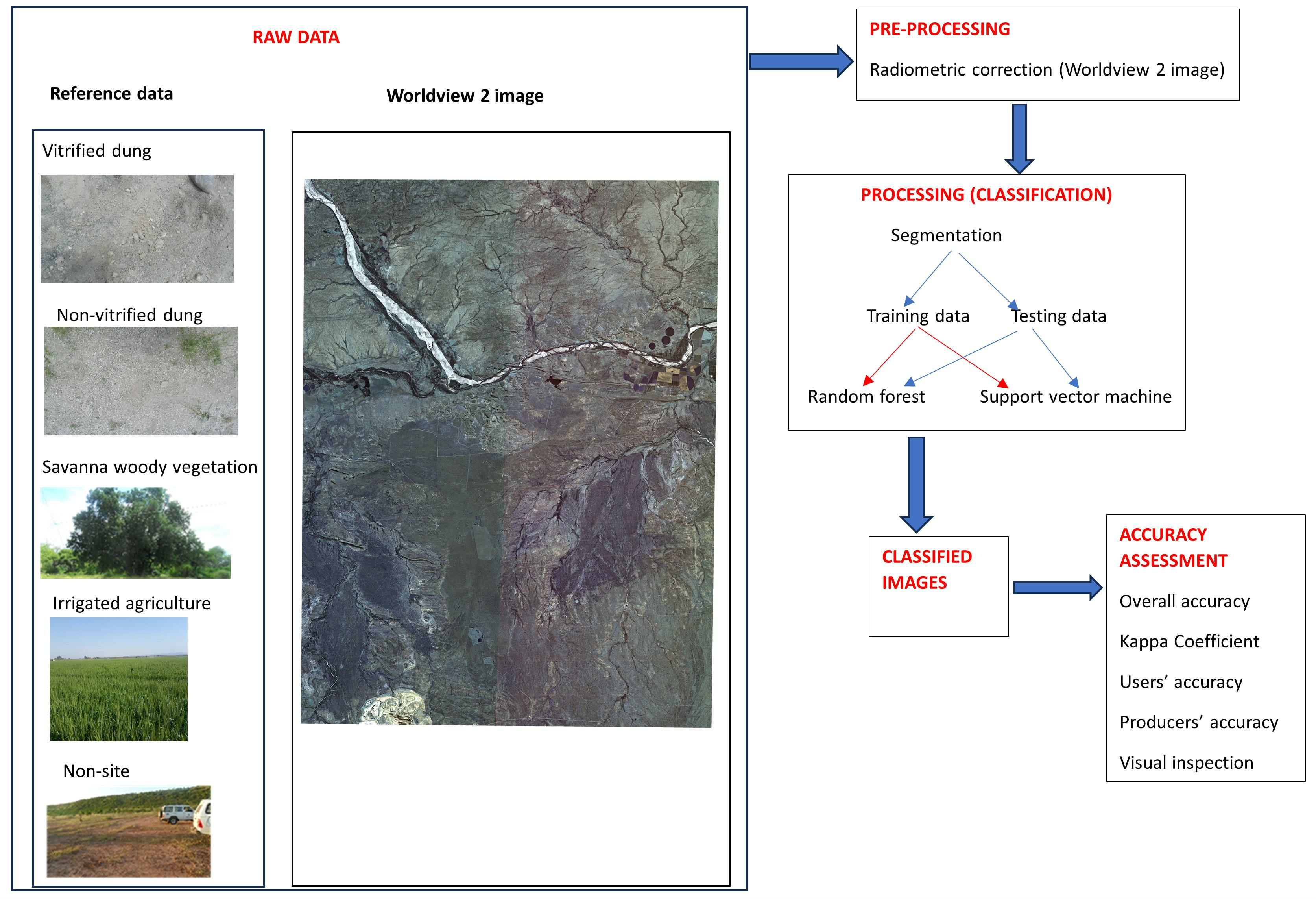
2. Materials and Methods

2.1. The Study Area and Archaeological Context

This study was carried out in the Mapungubwe Cultural Landscape, which is situated at the confluence of the Limpopo and Shashi rivers in Southern Africa (Figure 1). The landscape is listed under UNESCO World Heritage and is believed to have been occupied by one of the earliest complex societies in Southern Africa [47]. The Mapungubwe cultural landscape has been inundated with archaeological research since the early 1930s, with the discovery of the golden rhinoceros on Mapungubwe Hill [48,49]. These include one of the most extended systematic field walking surveys in the Mapungubwe landscape under the ‘Origins of Mapungubwe Project’ spanning more than two decades and discovering over 1100 farming community sites in the process [48]. Research has also revealed a lot of the archaeological materials that formed an integral part of everyday life and social patterns within the settlement. These include artefacts such as glass beads, bangles, ceramic figurines, and pots together with features such as middens and byres [50,51,52,53]. The byres are likely the centre of the settlement. This is because research has shown that the societies which occupied the Mapungubwe landscape practised the Central Cattle Pattern (CCP) settlement system, whereby the central space of the settlement housed the animal byre (kraal) in proximity to the male gathering area [47,54]. The byres are of two types, with one type having vitrified deposits while the other has non-vitrified/unburned dung deposits [49,55]. Vitrified dung is formed when thick dung deposits burn at about 1100 °C forming a glassy biomass slag [56,57]. However, there is no consensus on the cause of the above-mentioned burning—some researchers [55,56] attribute it to intentional causes, while others posit that it was accidental occurrences such as wildfires or lightning at very high temperatures [57]. Furthermore, the level of vitrification varies across the sites depending on the conditions under which the dung was burned. Some deposits depict a high degree of vitrification, while others are not fully vitrified or depict a mixture of vitrified dung and non-vitrified dung. Huffman et al., [55] postulates that a high level of vitrification is mostly found along the fence where there is wood, and the thickness of the vitrified layer reduces as one moves to the centre of the byre. This then leaves most of the vitrified dung sites with a combination of non-vitrified and vitrified dung deposits, depending on the degree of vitrification. However, this study investigates the feasibility of using GEOBIA to detect archaeological sites with vitrified dung and non-vitrified dung deposits in the SLCA. Although Cenchrus cilliaris has been previously used as an indicator of the aforementioned sites in central Eastern Botswana by Denbow [58], it is not a diagnostic feature of the sites in SLCA. As a result, this study targeted bare sites.

2.2. Worldview-2

Two cloud-free WorldView-2 images captured on 5 August 2014, covering 1388 km2 of the study area, at spatial resolutions of 0.5 m and 2 m for the panchromatic band and multispectral bands, respectively, were used in this study. This is the best period to identify the surface of archaeological features because the vegetation has lost leaves and grasses have died, leaving most of the archaeological dung deposits uncovered (Southern hemisphere spring season). The images were obtained from Digital Globe and were geometrically corrected on supply. WorldView-2 satellite collects images in one panchromatic (450–800 nm) and eight multispectral bands at 400–450 nm (B1-coastal), 450–510 nm (B2-blue), 510–581 nm (B3-green), 585–625 nm (B4-yellow), 630–690 nm (B5-red), 705–745 nm (B6-red edge), 770–895 nm (B7-near infrared-1), and 860–1040 nm (B8-near-infrared-2). Nonetheless, the panchromatic band was excluded from the analysis in this study. The Fast Line-of-Sight Atmospheric Analysis of Hypercubes (FLAASH) tool in Envi 4.8 software was used to perform radiometric corrections on each image before they were merged.

2.3. Segmentation and Feature Selection

Image segmentation creates the objects, which are the basic spatial units of analysis in GEOBIA [33]. The created objects relate to natural spatial units; therefore, they should form a meaningful spatial unit for land cover classification [36,59]. Moreover, the quality of demarcation of target objects directly impacts the accuracy rate for predicting classes in an image [33]. Multi-resolution segmentation (MRS) algorithm in 64-bit Ecognition developer v.9 software, was used in this study. This is the most regularly used segmentation technique [60] and researchers [10,61,62] have held it as one of the best segmentation methods in GEOBIA. MRS employs a bottom–up region method, whereby a pixel is identified as a single object before being paired with other spatially adjacent objects to form bigger objects, depending mainly on the defined scale heterogeneity level [10,63]. The object pairing is entrenched in the pairwise clustering procedure [64]. The MRS gives the user an opportunity to regulate the magnitude of homogeneity within the objects by setting the scale, shape, and colour parameters [65].
The scale parameter significantly affects the quality of the segmentation procedure because it determines the extent of the object which can, in turn, lead to under-segmentation or over-segmentation error [15]. The large values for scale parameter allow for the creation of large objects and more heterogeneity within the objects while small values for scale create small homogeneous objects. The impact of the segmentation scale on class distinction was investigated at 10 different scales (10, 20, 30, 40, 50, 60, 70, 80, 90, and 100) in this study. After finding the suitable scale factor, the shape and colour parameters were adjusted to improve the features of output image objects [36,63]. The shape is based on the geometric characteristics of the archaeological and non-archaeological features. The shape of an object is influenced by two inversely proportional properties, which are smoothness and compactness [66,67]. The colour parameter deals with spectral heterogeneity of archaeological and non-archaeological features, as a result, it is affected by the weight assigned to each band in segmentation [10,63]. However, the weight value of each band was left at one, which is the default, to avoid biases in the classification. The combined weighted values of shape and colour parameters add up to a total of one [10,67]. Studies by Costa et al. [59] and Mathieu et al. [63] have shown that in most cases desired results are achieved when the shape is given less weight than colour. As a result, in tuning the parameters for segmentation in this study, the shape parameter was always given less value than colour in order to give more weight to spectrally homogenous pixels when segmenting. To identify the optimum image segments using the abovementioned parameters, studies have used the trial-and-error method by varying their values [13,35,39,63,68]. The image segmentation procedure is, therefore, performed when the objects produced visually match the real-world features of interest. Consequently, in identifying the optimum segments in this study, the trial-and-error method assessed through visual inspection was used to regulate the scale, shape, and colour parameters in segmentation. The scale parameter of 50 and the shape parameter of 0.2 were chosen as the optimum segmentation parameters in this study.
After image object segmentation, the variable selection was carried out for use in object-based classification. Variable feature selection procedure identifies a subset of optimum object features that will produce the best results in the classification process [32,69]. The classification process can comprise numerous object feature properties ranging from context, size, spectral data, texture, and shape [32,33]. The feature selection process can be executed in two ways by either using software algorithms or a manual process based on literature reviews and expert knowledge [12,35,69,70]. In this study, several object characteristics were manually assessed based on a literature review and expert knowledge in an attempt to identify the best subset of features for classification [12,71]. All the object features used as input variables in this study are listed in Table 1. Image objects were spectrally differentiated using the mean spectral value of each band computed at the object level. To differentiate image objects with information extracted from their geometric features, the area extent of the image objects was used. The area extent of an object is measured by counting the pixels within it. This was carried out to differentiate objects of different sizes with similar spectral properties, such as river sand and vitrified dung sites [20]. Other various object characteristics and parameter settings, such as shape, texture, and class-related features, were explored but did not produce suitable outcomes.

2.4. Image Classification

2.4.1. Random Forest

RF classifier was used to map the archaeological sites and other LULC cover types using the classes created on the segments. Since its inception by Breiman [72], RF has been effectively used in several domains like pharmacology [73,74], medical imaging [75,76,77], and genetics [78,79,80] because of its intrinsic ability to measure variable importance and its robust predictive power. Furthermore, throughout the last decade, there was a surge in the use of RF in different remote sensing applications, such as vegetation species mapping [81,82,83], agriculture [84,85], and archaeology [20,86].
RF is pronounced as a group of classifiers that generates binary decision trees and allocates class according to popular votes on each node [87]. RF grows each tree using a different bootstrapped sample drawn from the training data, with about a third of the training data not being included in building each tree [72,88]. The left-out sample, commonly known as the out-of-bag (OOB), is then used to evaluate the significance of each variable in classification and generalisation error [88,89]. RF classification was carried out using the randomForest package within the R statistical environment [90]. Training the RF classifier encompasses optimising two parameters: (1) the number of variables used in a dataset to split trees at each node (mmtry) and (2) the number of trees in the forest (ntree) [90,91]. Following earlier studies [83,92,93], this study used a grid search approach based on the OOB estimate of error to look for the best pair of both mtry and ntree parameters. The values for mtry and ntree were assessed from 1 to 9 and 500 to 9500 with an interval of 1000, respectively.

2.4.2. Support Vector Machines

SVM is a non-parametric supervised classifier that is gaining wide use in remote sensing because of its ability to achieve good generalisations even with inadequate training data [94,95,96]. The SVM model was initiated by Vapnik and Chervonenkis [97] before it was fully discussed by Vapnik [98]. In general, SVMs are linear classifiers that are composed of hyperplanes that separate data classes via the largest margin within a high dimensional feature space [99,100]. The user chooses the SVM kernel function to be used for the training process that picks support vectors along the hyperplane surface [101]. The radial basis function (RBF) kernel was selected for classification in this study. RBF has been applied to numerous LULC classifications where it achieved higher classification accuracies than other SVM kernels and classification algorithms [100]. This is also supported by the results from Pal and Mather [102], who found out that RBF outperformed other classification algorithms in classifying land cover data. This might be largely because of its ability to handle non-linear relationships concerning class labels and attributes, which is mostly the case with spatial data [99]. In this study, the RBF classification process involved the identification of optimal values of regularisation parameter sigma (C) and the width of the kernel gamma (γ) that are suitable for discriminating archaeological and non-archaeological classes [99,100,103]. The optimisation for the optimum combination of γ and C parameter values was carried out using a 10-fold cross-validation and grid search. The grid search procedure assesses various pairs of cost and gamma parameters and picks the one with the lowest cross-validation error [104,105]. The optimisation of RBF parameters and classification used e1071 and caret libraries of R statistical packages, respectively.

2.4.3. Reference Data and Accuracy Assessment

Mapping of ground reference points to be used in image classification was carried out in September 2016, after initially visiting the Mapungubwe cultural landscape in September 2015 with an archaeological expert. The short time lapse between the date of image capture and reference points collection has no bearing on the classification outcome of this study because the chemical composition and structure of the targeted deposits take a long time to change [55]. Data was collected during spring, which is also the season when the images were captured, when most of the landscape is bare, thus, revealing archaeological materials on the surface. Furthermore, the land use changes in the chosen study area are minimal because it is legally protected by national laws as a national park and a game reserve and by the United Nations Educational, Scientific and Cultural Organisation as a Cultural Landscape.
Data collection was carried out using a purposive sampling technique whereby only vitrified dung and non-vitrified dung deposit sites appearing in the literature and dating to the period of interest were targeted. The coordinates for the identified sites were acquired from a site register developed by Huffman [51,52], and their location was tracked using a handheld global positioning system device (GPS). Additionally, three more LULC classes composed of irrigated agriculture (pivot agriculture), savannah woody vegetation, and bare land (natural soils) identified during fieldwork were added as variables during the image classification process. The savannah woody vegetation represented the natural vegetation within the study area, while pivot irrigation farms were classified as irrigated agriculture. The focus of the study is to differentiate archaeological deposits, non-archaeological deposits, and vegetation in general; therefore, a broad categorisation of vegetation species is deemed acceptable, because individual vegetation species are not important in this study. For general LULC, we used our expert knowledge of the features in the study area to randomly select additional objects for each class through the visual inspection of a pan-sharpened WV image. In sum, 394 objects were chosen, of which 17 belonged to vitrified dung, 114 non-vitrified dung, 36 irrigated agriculture, 114 non-sites, and 114 savannah woody vegetation. The variation in class sizes was largely due to the differences in the areas covered by each class, with vitrified dung being the least prevalent in the study area.
The accuracy assessment in GEOBIA is a contested terrain, with some studies [106,107] arguing that the shape of the segment influences the overall classification accuracy of the model. On the other hand, research [14] demonstrated that the accuracy of the shape of the segment has no significant impact on the classification accuracy of the models. The accuracy assessment in this study is focused on the location accuracy of the objects rather than the accuracy of their shape in relation to ground features. This is because the high erosion, which is prevalent in the area, has led to instances where vitrified dung and non-vitrified dung get mixed, or one gets coated with the other depending on which one is in the direction of erosion. The quality of thematic maps created using RF and SVM classification algorithms was evaluated using a dataset that was randomly generated by splitting the ground-referenced data for the study area into 70% and 30% for training and validation, respectively, before running the classification model. This resulted in 117 polygons spread across the entire study area, with class sizes varying from 5 to 34 polygons being chosen for validation. This is because the polygons are the basic spatial units for the thematic maps created from the segments. This method was applied as it permits the assessment of the whole classification process, beginning with the segmentation. Some statistical analysis, which includes overall accuracy, user’s accuracy, and producer’s accuracy, were then performed as a way of assessing the reliability of the maps generated for a site survey. The layout plans of archaeological sites drawn by Huffman [53] and Calabrese [108] were overlaid on the matching predicted sites to visually evaluate the accuracy of the above-mentioned classifiers in detecting site extent together with the distribution of archaeological and non-archaeological features within a site.

3. Results

3.1. Image Segmentation

The optimum image segments were identified by varying the values for scale, colour, and shape based on a trial-and-error approach. The results demonstrated that segmentation performed using the scale, shape, and colour parameters of 50, 0.2, and 0.8, respectively, produced accurate boundaries of geographic features (Figure 2). The segmentation process produced 5,189,584 objects.

3.2. Tuning RF and SVM Parameters

The RF algorithm parameters were optimised to predict archaeological classes using a grid search procedure, and the results have shown that a combination of a mtry value of 5 and a ntree value of 500 produced the lowest OOB error rate of 0.059 (Figure 3). The highest OOB error rates (0.072) were produced by combinations of mtry values of 9 and ntree values of 500 and 1500.
The best-input parameters for classification using RBF in SVM were determined using 10-fold cross-validation and grid search. The optimisation results have demonstrated that the C l o g 10 ( 100 ) and γ ( l o g 10 ( 0.01 ) ) are the best input parameters for predicting archaeological classes using RBF in the SVM classifier (Figure 4). The combination of the optimal C (100) and γ (0.01) produced the lowest cross-validation error of 0.036. The highest cross-validation error (0.8) was attained when C was set to l o g 10 ( o . 1 ) and γ was set to l o g 10 ( 1000 ) see Figure 4.

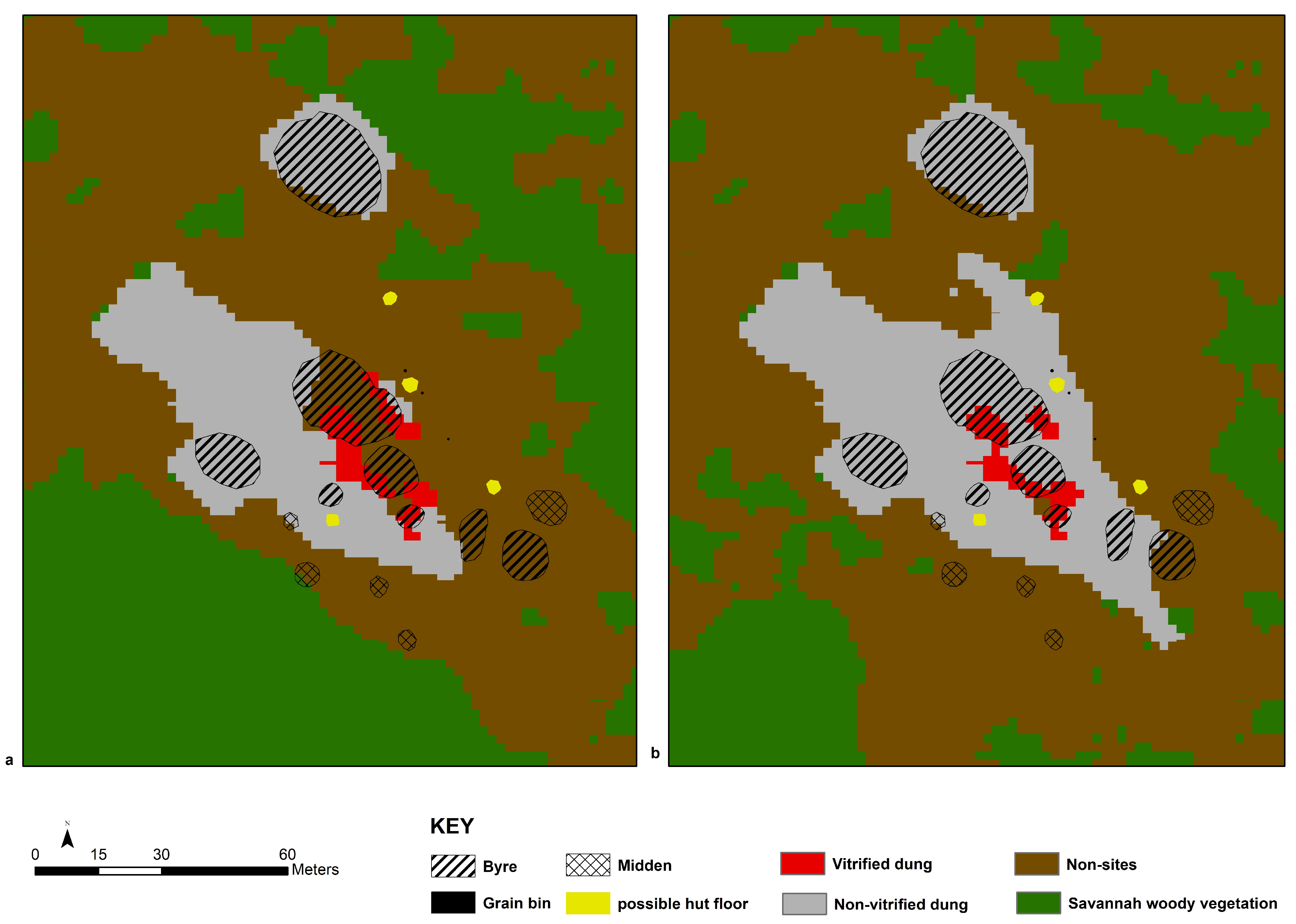
3.3. Image Classification and Site Prediction

GEOBIA classification carried out using RF and SVM algorithms defined non-sites, savannah woody vegetation, irrigated agriculture, vitrified dung, and non-vitrified dung across the study area, as shown in Figure 5. Non-sites cover large parts of the study area, followed by savannah woody vegetation, while other classes cover very small portions of the study area. A visual inspection of the predictive maps of RF and SVM shows that the two classifiers have correctly predicted the locations of known archaeological sites (Figure 5). However, there was a difference in how the two classifiers predicted the non-sites, savannah woody vegetation, irrigated agriculture, vitrified dung, and non-vitrified dung sites across the study area (Figure 5 and Table 2). Non-sites on a map predicted by SVM (878 km2) covered a large area when compared to the one predicted by RF (812.10 km2). On the other hand, the map produced by RF (19.74 km2) indicates the spread of non-vitrified dung over large portions of the study area than the one on the map produced by SVM (13.28 km2). The map predicted by RF shows that non-vitrified dung sites are widely spread in the northern parts of the study area when compared to the one produced by SVM.

3.4. Accuracy Assessment

The prediction accuracies for RF and SVM classification algorithms were assessed using 117 holdout polygons created by partitioning reference data into training (70%) and verification (30%). Overall, SVM achieved higher classification accuracies than the RF (Table 3 and Table 4). SVM achieved an overall classification accuracy of 96.58% and a kappa coefficient of 0.9536, while the overall accuracy and kappa coefficient achieved by RF were 94.87% and 0.9305, respectively. Concerning the individual classes, a comparison between the SVM and RF algorithms shows that they achieved similar results for user’s and producer’s accuracies in most classes (Table 3 and Table 4). Vitrified dung achieved the lowest producer’s and user’s accuracies of 80% each in both RF and SVM algorithms. Irrigated agriculture and savannah woody vegetation achieved the highest user’s and producer’s accuracies of 100% each in both SVM and RF. The differences in the user’s and producer’s accuracies for the two abovementioned classifiers were noted in the classification of non-sites and non-vitrified dung classes. Two non-vitrified dung sites were confused with other classes, one with vitrified dung and the other confused with non-sites in RF (Table 4). However, in SVM classification, the confusion occurred in only one non-vitrified dung site, which was misclassified as vitrified dung (Table 3).
The outlines of the sites mapped were also used to gauge the accuracy of the RF and SVM models in classifying non-vitrified dung and vitrified dung deposits (Figure 6 and Figure 7). However, the sizes of sites predicted by the RF and SVM models in places that are potentially vulnerable to erosion are covering a larger area extent than the plans drawn by both Huffman [53], see Figure 6, and Calabrese [108], see Figure 7. Generally, the SVM model picked larger extents of non-vitrified dung than the RF model in most sites (Figure 6 and Figure 7). Additionally, some of the byres mapped by Calabrese [108] were not detected by the SVM and RF models (Figure 7). The two abovementioned models also classified other archaeological features, such as dagga, middens, and grain bins, as non-sites.

4. Discussion

The monitoring and prospection of archaeological sites using remote sensing techniques entrenched on the variations in the spectral reflectance of archaeological features and their surroundings are widely becoming a common practice [4,19,25,109]. Even though high classification accuracies have been achieved, some challenges in relation to subtle spectral differences between archaeological features and their surroundings have been reported [7,29]. Areas characterised by archaeological features that were constructed using local materials or are covered with tracts of eroded archaeological material normally share spectral signatures with archaeological features in their locality [7,29]. This challenge becomes a major limitation when using methods such as pixel-based techniques because they depend solely on spectral signatures to classify remote sensing data [29,110], consequently restricting the application of remote sensing techniques in archaeology to areas with detectable spectral variations between archaeological features and non-archaeological features. The solution, thus, lies in using classification approaches that can integrate spatial and spectral data in their process [15,33,36,110]. Hence, the main intention of this study was to assess the possibility of discriminating non-vitrified dung, vitrified dung, and non-sites using their spatial and spectral data as input variables in GEOBIA models based on advanced classification algorithms (RF and SVM). Furthermore, the classification outcomes of this study were assessed using confusion matrices and visual inspection.
Results of this study have shown that GEOBIA based on SVM and RF classifiers can differentiate archaeological and non-archaeological features, even in environments where there are different features with spectral homogeneity. The aforementioned success in the classification attained using GEOBIA can mainly be credited to its utilisation of spatial attributes to compensate for the spectral homogeneity of various features [33]. The high spatial resolution of the WorldView-2 images used in this study clearly defined the extent of each site, thus facilitating the incorporation of the area extent of the individual image objects into classification models. The image objects depicting non-sites were generally larger than those depicting the vitrified dung sites. This enabled the classification models to discern vitrified dung from non-sites, especially along the river where there is spectral confusion. This was a great improvement compared to the pixel-based classification performed by Thabeng et al. [20], where features such as rivers were confused with vitrified dung sites due to their spectral similarities. Our findings concur with those of Hu et al. [35], who successfully incorporated area as a spatial attribute to differentiate spectrally homogenous but spatially different features, such as rivers and lakes. Despite the findings of the earlier studies [111], this study proves that GEOBIA models can achieve positive results in archaeological applications, even when the shape is not one of the site spatial characteristics used as input variables. This is because the outlines of most sites are deformed by post-depositional processes.
The error matrix accuracy assessment of the GEOBIA-based RF and SVM algorithms has shown that they both generally achieved high overall classification accuracies and kappa coefficients. This is consistent with other studies [10,39,112,113], which attained high classification accuracies when using GEOBIA based on SVM and RF classification algorithms to delineate features in complex landscapes. However, errors of commission and omission for vitrified dung sites and non-vitrified dung sites are higher in the GEOBIA models used in this study when compared to the pixel-based approach used by Thabeng et al. [20]. This might be because GEOBIA does not rely on a single pixel value as is the case in pixel-based classification but uses a combination of spatial attributes and averages of spectral values of an object for prediction. Furthermore, some of the dung deposits do not completely vitrify, while in some instances, erosion causes vitrified dung to coat non-vitrified dung or vice versa. As such, this leaves a thin line between vitrified and non-vitrified dung deposits on the landscape, resulting in the confusion between vitrified and non-vitrified dung deposits. A comparison of the two GEOBIA classifiers used in this study reveals that SVM outclassed RF in user’s and producer’s accuracies of non-vitrified dung, savannah woody vegetation, non-sites, and irrigated agriculture (Table 3 and Table 4). In general, this was a great improvement from the results of pixel-based SVM classification carried out by Thabeng et al. [18], where RF showed better overall performances than SVM. In contrast, the performance of RF generally decreased in GEOBIA when compared against the pixel-based approach [20]. Our results for this study support those of Kavzoglu et al. [114], who found that SVM outperforms RF in GEOBIA models.
Furthermore, when overlaid on the layouts of the sites, there were variations in how RF and SVM classifiers predicted the extent of individual archaeological sites (Figure 6 and Figure 7). SVM classifier detected areas possibly covered with thin layers of eroded materials from non-vitrified dung deposits, whereas RF only picked thick non-vitrified dung deposits. As a result, the sizes of the sites predicted by the RF and SVM models are not a true representative of their original extent [53,108]. However, the aforementioned variations in the accuracies of the RF and SVM models can complementarily be used to survey for archaeological sites, as suggested by Thabeng et al. [20]. Generally, the visual inspection of the classifications produced by both RF and SVM models has shown that non-vitrified dung covers large areas, and it always surrounds the deposits of vitrified dung. This supports the findings of Huffman et al. [55], who posits that not all dung vitrifies during the vitrification process. Moreover, some of the byres mapped by Calabrese [108] were not detected by the models possibly because all of their materials have been eroded. This is in line with the findings of Calabrese [108], who posits that the majority of the sites are in danger of being extinct because of the erosion which is rampant in the area. Other archaeological features that the models could not detect include the middens, possibly because they had been eroded.
A visual inspection of the classification results also demonstrates that both maps depict a moderately accurate representation of the LULC classes of interest within the study area. In general, both classifiers accurately predicted the archaeological sites characterised by non-vitrified dung and vitrified dung. However, there are differences in the classification accuracies of the RF and SVM classifiers, especially in the prediction of non-vitrified dung deposits in the northern part of the study area. The non-vitrified dung class appears to be well represented by the SVM classifier in GEOBIA. For example, SVM depicts less confusion between non-vitrified dung and non-sites in the northern part of the study area (Figure 5). The fact that GEOBIA reduces within-class spectral heterogeneity by using spectral values means of an object in classification might have contributed to the betterment of SVM classification accuracies in this study. The aforementioned assertion is in agreement with the findings of Maxwell [115], that the classification accuracies of SVM improve when mean spectral values are used in the classification process. Despite less emphasis on the geometric accuracy of segmentation results, GEOBIA achieved better classification accuracies than pixel-based classification when predicting vitrified dung, non-vitrified dung, and non-sites in the SLCA [20]. Our findings are similar to those of Myint et al. [15], who found that GEOBIA performs better than pixel-based classification. Additionally, the outcomes of this study further support the findings of Belgiu and Drǎguţ [14], that the segmentation output has less impact on the accuracy of the classification models. The success of the method presented in this study will help researchers and heritage managers extend the utilisation of remote sensing techniques to areas where there are subtle spectral contrasts between archaeological features and their surroundings. In addition, employing remote sensing techniques will also assist the researchers and heritage managers in surveying and monitoring archaeological sites in huge and remote areas over a short period [4,25,109,116]. In summary, we acknowledge that this study had some limitations, which resulted in confusion between classes, especially non-vitrified dung and non-sites in the northern part of the study area. The aforementioned limitations can be linked to the inability to gather data in the near-infrared regions, which are sensitive to the soil chromosomes due to the satellite sensor used. A possible solution to the above problem is the fusion of data from high spectral resolution and high spatial resolution sensors.

5. Conclusions

The findings of this research have shown that GEOBIA based on RF and SVM classifiers accurately discriminate amongst the archaeological deposits and non-archaeological deposits in the SLCA. The GEOBIA managed the spectral confusion between archaeological and non-archaeological features, such as vitrified dung deposits and non-sites, by combining their spatial and spectral attributes in the classification process. Even though SVM generally outperformed RF, both classifiers attained high prediction accuracies. Therefore, this means that both classifiers should be considered reliable predictors of archaeological sites with vitrified dung and non-vitrified dung deposits. In summary, this study demonstrated the capabilities of the GEOBIA method in mapping surface archaeological features, especially those with similar spectral characteristics to other objects in their surroundings, which is a common challenge in the use of remote sensing in archaeology.
The ability to map archaeological features which have similar spectral properties to their surroundings by the GEOBIA method will help researchers and heritage managers to expand archaeological remote sensing surveys to areas where it was impossible to carry them out before because of a lack of spectral contrast between features. Additionally, the use of remote sensing applications will help researchers and heritage resources managers carry out fast, cheap, and systematic regional archaeological site surveys and monitoring, especially when considering the challenges and risks one has to face when carrying out foot surveys in certain areas of the world.

Author Contributions

Conceptualization, O.L.T., E.A. and S.M.; methodology, O.L.T., E.A. and S.M.; software, O.L.T. and E.A.; validation, O.L.T., S.M. and E.A.; formal analysis, O.L.T.; investigation, O.L.T., S.M. and E.A.; resources, S.M. and E.A.; data curation, O.L.T.; writing—original draft preparation, O.L.T.; writing—review and editing, E.A. and S.M.; visualization, O.L.T.; supervision, E.A. and S.M.; project administration, O.L.T.; funding acquisition, O.L.T. All authors have read and agreed to the published version of the manuscript.

Funding

The University of Botswana training department and Digital Globe Foundation funded this research.

Data Availability Statement

Data sharing is not possible due to licensing restrictions from third parties.

Acknowledgments

We appreciate the invaluable support we obtained from SANParks who let us into Mapungubwe National Park, and the assistance offered by its members of staff. We thank the DeBeers Group for accommodating us at Venetia Research Centre and permitting us to look for archaeological sites in the Venetia Nature Reserve. We also thank the Venetia staff for protecting us during the survey in the reserve and Thomas Huffman for sharing his data and taking us around the study area.

Conflicts of Interest

Authors declare no conflict of interest.

References

  1. Adam, E.; Mutanga, O.; Odindi, J.; Abdel-Rahman, E.M. Land-use/cover classification in a heterogeneous coastal landscape using RapidEye imagery: Evaluating the performance of random forest and support vector machines classifiers. Int. J. Remote Sens. 2014, 35, 3440–3458. [Google Scholar] [CrossRef]
  2. Adam, E.; Mutanga, O.; Rugege, D.; Ismail, R. Discriminating the papyrus vegetation (Cyperus papyrus L.) and its co-existent species using random forest and hyperspectral data resampled to HYMAP. Int. J. Remote Sens. 2012, 33, 552–569. [Google Scholar] [CrossRef]
  3. Aguilar, M.A.; Novelli, A.; Nemamoui, A.; Aguilar, F.J.; Lorca, A.G.; González-Yebra, Ó. Optimizing multiresolution segmentation for extracting plastic greenhouses from WorldView-3 imagery. In Proceedings of the 10th International KES Conference on Intelligent Interactive Multimedia: Systems and Services, KES-IIMSS-17, Vilamoura, Portugal, 21–23 June 2017; pp. 31–40. [Google Scholar]
  4. Ahmed, A.A.; Kalantar, B.; Pradhan, B.; Mansor, S.; Sameen, M.I. Land Use and Land Cover Mapping Using Rule-Based Classification in Karbala City, Iraq. In GCEC 2017: Proceedings of the 1st Global Civil Engineering Conference; Pradhan, B., Ed.; Springer: Singapore, 2017; pp. 1019–1027. [Google Scholar]
  5. Alexakis, D.; Sarris, A.; Astaras, T.; Albanakis, K. Detection of Neolithic settlements in Thessaly (Greece) through multispectral and hyperspectral satellite imagery. Sensors 2009, 9, 1167–1187. [Google Scholar] [CrossRef] [PubMed]
  6. Aqdus, S.A.; Hanson, W.S.; Drummond, J. The potential of hyperspectral and multi-spectral imagery to enhance archaeological cropmark detection: A comparative study. J. Archaeol. Sci. 2012, 39, 1915–1924. [Google Scholar] [CrossRef]
  7. Beck, A.R. Archaeological Site Detection: The Importance of Contrast. In Proceedings of the 2007 Annual Conference of the Remote Sensing and Photogrammetry Society, Newcastle Upon Tyne, UK, 11–14 September 2007; pp. 307–312. [Google Scholar]
  8. Beck, A.R.; Philip, G.; Abdulkarim, M.; Donoghue, D. Evaluation of Corona and Ikonos high resolution satellite imagery for archaeological prospection in western Syria. Antiquity 2007, 81, 161–175. [Google Scholar] [CrossRef]
  9. Belgiu, M.; Csillik, O. Sentinel-2 cropland mapping using pixel-based and object-based time-weighted dynamic time warping analysis. Remote Sens. Environ. 2018, 204, 509–523. [Google Scholar] [CrossRef]
  10. Belgiu, M.; Drǎguţ, L. Comparing supervised and unsupervised multiresolution segmentation approaches for extracting buildings from very high resolution imagery. ISPRS J. Photogramm. Remote Sens. 2014, 96, 67–75. [Google Scholar] [CrossRef]
  11. Belgiu, M.; Drăguţ, L. Random forest in remote sensing: A review of applications and future directions. ISPRS J. Photogramm. Remote Sens. 2016, 114, 24–31. [Google Scholar] [CrossRef]
  12. Bennett, R.; Welham, K.; Hill, R.A.; Ford, A.L.J. The application of vegetation indices for the prospection of archaeological features in grass-dominated environments. Archaeol. Prospect. 2012, 19, 209–218. [Google Scholar] [CrossRef]
  13. Biagetti, S.; Merlo, S.; Adam, E.; Lobo, A.; Conesa, F.C.; Knight, J.; Bekrani, H.; Crema, E.R.; Alcaina-Mateos, J.; Madella, M. High and medium resolution satellite imagery to evaluate late holocene human–environment interactions in arid lands: A case study from the central Sahara. Remote Sens. 2017, 9, 351. [Google Scholar] [CrossRef]
  14. Blaschke, T. Object based image analysis for remote sensing. ISPRS J. Photogramm. Remote Sens. 2010, 65, 2–16. [Google Scholar] [CrossRef]
  15. Blaschke, T.; Hay, G.J.; Kelly, M.; Lang, S.; Hofmann, P.; Addink, E.; Feitosa, R.Q.; Van der Meer, F.; Van der Werff, H.; Van Coillie, F. Geographic object-based image analysis–towards a new paradigm. ISPRS J. Photogramm. Remote Sens. 2014, 87, 180–191. [Google Scholar] [CrossRef] [PubMed]
  16. Blaschke, T.; Strobl, J. What’s wrong with pixels? Some recent developments interfacing remote sensing and GIS. Geo Inf. Syst. 2001, 14, 12–17. [Google Scholar]
  17. Boulesteix, A.-L.; Janitza, S.; Kruppa, J.; König, I.R. Overview of random forest methodology and practical guidance with emphasis on computational biology and bioinformatics. Wiley Interdiscip. Rev. Data Min. Knowl. Discov. 2012, 2, 493–507. [Google Scholar] [CrossRef]
  18. Breiman, L. Random forests. Mach. Learn. 2001, 45, 5–32. [Google Scholar] [CrossRef]
  19. Breiman, L.; Cutler, A. Random Forests-Classification Description. Department of Statistics, Berkeley. 2007. Available online: https://www.stat.berkeley.edu/~breiman/RandomForests/cc_home.htm (accessed on 19 October 2020).
  20. Calabrese, J.A. Report on the 1996 Field Season Shashi-Limpopo Archaeological Project; Prepared for DeBeers Consolidated Mines and the National Monuments Council. 1997; Unpublished.
  21. Cavalli, R.M.; Colosi, F.; Palombo, A.; Pignatti, S.; Poscolieri, M. Remote hyperspectral imagery as a support to archaeological prospection. J. Cult. Herit. 2007, 8, 272–283. [Google Scholar] [CrossRef]
  22. Chan, J.C.-W.; Paelinckx, D. Evaluation of Random Forest and Adaboost tree-based ensemble classification and spectral band selection for ecotope mapping using airborne hyperspectral imagery. Remote Sens. Environ. 2008, 112, 2999–3011. [Google Scholar] [CrossRef]
  23. Ciminale, M.; Gallo, D.; Lasaponara, R.; Masini, N. A multiscale approach for reconstructing archaeological landscapes: Applications in Northern Apulia (Italy). Archaeol. Prospect. 2009, 16, 143–153. [Google Scholar] [CrossRef]
  24. Clark, C.D.; Garrod, S.M.; Pearson, M.P. Landscape archaeology and remote sensing in southern Madagascar. Int. J. Remote Sens. 1998, 19, 1461–1477. [Google Scholar] [CrossRef]
  25. Corrie, R.K. Detection of Ancient Egyptian Archaeological Sites Using Satellite Remote Sensing and Digital Image Processing. In Earth Resources and Environmental Remote Sensing/GIS Applications II; 81811B-81811B-19; SPIE: Cergy, France, 2011. [Google Scholar] [CrossRef]
  26. Costa, H.; Foody, G.M.; Boyd, D.S. Using mixed objects in the training of object-based image classifications. Remote Sens. Environ. 2017, 190, 188–197. [Google Scholar] [CrossRef]
  27. Dalponte, M.; Bruzzone, L.; Gianelle, D. Fusion of Hyperspectral and LIDAR Remote Sensing Data for Classification of Complex Forest Areas. IEEE Trans. Geosci. Remote Sens. 2008, 46, 1416–1427. [Google Scholar] [CrossRef]
  28. Davis, D.S.; Douglass, K. Aerial and Spaceborne Remote Sensing in African Archaeology: A Review of Current Research and Potential Future Avenues. Afr. Archaeol. Rev. 2020, 37, 9–24. [Google Scholar] [CrossRef]
  29. Davis, D.S.; Lipo, C.P.; Sanger, M.C. A comparison of automated object extraction methods for mound and shell-ring identification in coastal South Carolina. J. Archaeol. Sci. Rep. 2019, 23, 166–177. [Google Scholar] [CrossRef]
  30. De Laet, V.; Paulissen, E.; Waelkens, M. Methods for the extraction of archaeological features from very high-resolution Ikonos-2 remote sensing imagery, Hisar (southwest Turkey). J. Archaeol. Sci. 2007, 34, 830–841. [Google Scholar] [CrossRef]
  31. Denbow, J.R. Cenchrus ciliaris: An ecological indicator of Iron Age middens using aerial photography in eastern Botswana. South Afr. J. Sci. 1979, 75, 405–408. [Google Scholar]
  32. Díaz-Uriarte, R. GeneSrF and varSelRF: A web-based tool and R package for gene selection and classification using random forest. BMC Bioinform. 2007, 8, 328. [Google Scholar] [CrossRef]
  33. Doneus, M.; Verhoeven, G.; Atzberger, C.; Wess, M.; Ruš, M. New ways to extract archaeological information from hyperspectral pixels. J. Archaeol. Sci. 2014, 52, 84–96. [Google Scholar] [CrossRef]
  34. Duro, D.C.; Franklin, S.E.; Dubé, M.G. A comparison of pixel-based and object-based image analysis with selected machine learning algorithms for the classification of agricultural landscapes using SPOT-5 HRG imagery. Remote Sens. Environ. 2012, 118, 259–272. [Google Scholar] [CrossRef]
  35. Elliot, T.; Morse, R.; Smythe, D.; Norris, A. Evaluating machine learning techniques for archaeological lithic sourcing: A case study of flint in Britain. Sci. Rep. 2021, 11, 10197. [Google Scholar] [CrossRef] [PubMed]
  36. Esch, T.; Thiel, M.; Bock, M.; Roth, A.; Dech, S. Improvement of image segmentation accuracy based on multiscale optimization procedure. IEEE Geosci. Remote Sens. Lett. 2008, 5, 463–467. [Google Scholar] [CrossRef]
  37. Fernández-Blanco, E.; Aguiar-Pulido, V.; Munteanu, C.R.; Dorado, J. Random Forest classification based on star graph topological indices for antioxidant proteins. J. Theor. Biol. 2013, 317, 331–337. [Google Scholar] [CrossRef] [PubMed]
  38. Fisher, M.; Fradley, M.; Flohr, P.; Rouhani, B.; Simi, F. Ethical considerations for remote sensing and open data in relation to the endangered archaeology in the Middle East and North Africa project. Archaeol. Prospect. 2021, 28, 279–292. [Google Scholar] [CrossRef]
  39. Genuer, R.; Poggi, J.-M.; Tuleau-Malot, C. Variable selection using random forests. Pattern Recognit. Lett. 2010, 31, 2225–2236. [Google Scholar] [CrossRef]
  40. Gray, K.R.; Aljabar, P.; Heckemann, R.A.; Hammers, A.; Rueckert, D. Random forest-based similarity measures for multi-modal classification of Alzheimer’s disease. NeuroImage 2013, 65, 167–175. [Google Scholar] [CrossRef]
  41. Guan, H.; Li, J.; Chapman, M.; Deng, F.; Ji, Z.; Yang, X. Integration of orthoimagery and lidar data for object-based urban thematic mapping using random forests. Int. J. Remote Sens. 2013, 34, 5166–5186. [Google Scholar] [CrossRef]
  42. Hadjimitsis, D.G.; Themistocleous, K.; Agapiou, A.; Clayton, C.R.I. Monitoring archaeological site landscapes in Cyprus using multi-temporal atmospheric corrected image data. Int. J. Archit. Comput. 2009, 7, 121–138. [Google Scholar] [CrossRef]
  43. Hanisch, E.O.M. An Archaeological Interpretation of Certain Iron Age Sites in the Limpopo/Shashi Valley. Master’s Thesis, University of Pretoria, Pretoria, South Africa, 1980. [Google Scholar]
  44. Hanisch, E.O.M. Schroda: The archaeological evidence. In Sculptured in Clay: Iron Age Figurines from Schroda, Limpopo Province, South Africa; National Cultural History Museum: Pretoria, South Africa, 2002; pp. 20–39. [Google Scholar]
  45. Harrower, M.J.; D’Andrea, A.C. Landscapes of state formation: Geospatial analysis of Aksumite settlement patterns (Ethiopia). Afr. Archaeol. Rev. 2014, 31, 513–541. [Google Scholar] [CrossRef]
  46. Hsu, C.-W.; Chang, C.-C.; Lin, C.-J. A Practical Guide to Support Vector Classification; Department of Computer Science and Information Engineering: Taipei, Taiwan, 2003; Available online: https://www.csie.ntu.edu.tw/~cjlin/papers/guide/guide.pdf (accessed on 15 May 2019).
  47. Hu, Q.; Wu, W.; Xia, T.; Yu, Q.; Yang, P.; Li, Z.; Song, Q. Exploring the Use of Google Earth Imagery and Object-Based Methods in Land Use/Cover Mapping. Remote Sens. 2013, 5, 6026–6042. [Google Scholar] [CrossRef]
  48. Huang, C.; Davis, L.S.; Townshend, J.R.G. An assessment of support vector machines for land cover classification. Int. J. Remote Sens. 2002, 23, 725–749. [Google Scholar] [CrossRef]
  49. Huang, C.-L.; Liao, H.-C.; Chen, M.-C. Prediction model building and feature selection with support vector machines in breast cancer diagnosis. Expert Syst. Appl. 2008, 34, 578–587. [Google Scholar] [CrossRef]
  50. Huang, C.-L.; Wang, C.-J. A GA-based feature selection and parameters optimization for support vector machines. Expert Syst. Appl. 2006, 31, 231–240. [Google Scholar] [CrossRef]
  51. Huffman, T.N. Mapungubwe and Great Zimbabwe: The origin and spread of social complexity in southern Africa. J. Anthropol. Archaeol. 2009, 28, 37–54. [Google Scholar] [CrossRef]
  52. Huffman, T.N. Origins of Mapungubwe Project, Progress Report 2008 Prepared for De Beers, the NRF, SAHRA and SANParks; 2009; pp. 1–65; Unpublished report.
  53. Huffman, T.N. Origins of Mapungubwe Project, Progress Report 2011 Prepared for De Beers, the NRF, SAHRA and SANParks; 2011; pp. 1–35; Unpublished report.
  54. Huffman, T.N.; Du Piesanie, J. Khami and the Venda in the Mapungubwe landscape. J. Afr. Archaeol. 2011, 9, 189–206. [Google Scholar] [CrossRef]
  55. Huffman, T.N.; Elburg, M.; Watkeys, M. Vitrified cattle dung in the Iron Age of southern Africa. J. Archaeol. Sci. 2013, 40, 3553–3560. [Google Scholar] [CrossRef]
  56. Huffman, T.N.; Murimbika, M.; Schoeman, M.H. Origins of Mapungubwe Project, Progress Report 2004 Prepared for De Beers, the NRF, SAHRA and SANParks; 2004; pp. 1–21; Unpublished report.
  57. Immitzer, M.; Atzberger, C.; Koukal, T. Tree species classification with random forest using very high spatial resolution 8-band WorldView-2 satellite data. Remote Sens. 2012, 4, 2661–2693. [Google Scholar] [CrossRef]
  58. Jacquin, A.; Misakova, L.; Gay, M. A hybrid object-based classification approach for mapping urban sprawl in periurban environment. Landsc. Urban Plan. 2008, 84, 152–165. [Google Scholar] [CrossRef]
  59. Kavzoglu, T.; Colkesen, I. A kernel functions analysis for support vector machines for land cover classification. Int. J. Appl. Earth Obs. Geoinf. 2009, 11, 352–359. [Google Scholar] [CrossRef]
  60. Kavzoglu, T.; Colkesen, I.; Yomralioglu, T. Object-based classification with rotation forest ensemble learning algorithm using very-high-resolution WorldView-2 image. Remote Sens. Lett. 2015, 6, 834–843. [Google Scholar] [CrossRef]
  61. Kazmi, J.H.; Haase, D.; Shahzad, A.; Shaikh, S.; Zaidi, S.M.; Qureshi, S. Mapping spatial distribution of invasive alien species through satellite remote sensing in Karachi, Pakistan: An urban ecological perspective. Int. J. Environ. Sci. Technol. 2022, 19, 3637–3654. [Google Scholar] [CrossRef]
  62. Keay, S.J.; Parcak, S.H.; Strutt, K.D. High resolution space and ground-based remote sensing and implications for landscape archaeology: The case from Portus, Italy. J. Archaeol. Sci. 2014, 52, 277–292. [Google Scholar] [CrossRef]
  63. Lasaponara, R.; Leucci, G.; Masini, N.; Persico, R. Investigating archaeological looting using satellite images and GEORADAR: The experience in Lambayeque in North Peru. J. Archaeol. Sci. 2014, 42, 216–230. [Google Scholar] [CrossRef]
  64. Lasaponara, R.; Masini, N. QuickBird-based analysis for the spatial characterization of archaeological sites: Case study of the Monte Serico medieval village. Geophys. Res. Lett. 2005, 32, L12313. [Google Scholar] [CrossRef]
  65. Lasaponara, R.; Masini, N. Identification of archaeological buried remains based on the normalized difference vegetation index (NDVI) from quickbird satellite data. IEEE Geosci. Remote Sens. Lett. 2006, 3, 325–328. [Google Scholar] [CrossRef]
  66. Lebedev, A.V.; Westman, E.; Van Westen, G.J.P.; Kramberger, M.G.; Lundervold, A.; Aarsland, D.; Soininen, H.; Kłoszewska, I.; Mecocci, P.; Tsolaki, M. Random Forest ensembles for detection and prediction of Alzheimer’s disease with a good between-cohort robustness. NeuroImage Clin. 2014, 6, 115–125. [Google Scholar] [CrossRef]
  67. Li, M.; Ma, L.; Blaschke, T.; Cheng, L.; Tiede, D. A systematic comparison of different object-based classification techniques using high spatial resolution imagery in agricultural environments. Int. J. Appl. Earth Obs. Geoinf. 2016, 49, 87–98. [Google Scholar] [CrossRef]
  68. Li, Q.; Wang, C.; Zhang, B.; Lu, L. Object-based crop classification with Landsat-MODIS enhanced time-series data. Remote Sens. 2015, 7, 16091–16107. [Google Scholar] [CrossRef]
  69. Lin, F.; Yeh, C.-C.; Lee, M.-Y. The use of hybrid manifold learning and support vector machines in the prediction of business failure. Knowl. Based Syst. 2011, 24, 95–101. [Google Scholar] [CrossRef]
  70. Liu, M.; Liu, X.; Liu, D.; Ding, C.; Jiang, J. Multivariable integration method for estimating sea surface salinity in coastal waters from in situ data and remotely sensed data using random forest algorithm. Comput. Geosci. 2015, 75, 44–56. [Google Scholar] [CrossRef]
  71. Lu, D.; Weng, Q. A survey of image classification methods and techniques for improving classification performance. Int. J. Remote Sens. 2007, 28, 823–870. [Google Scholar] [CrossRef]
  72. Luo, H.; Wang, L.; Shao, Z.; Li, D. Development of a multi-scale object-based shadow detection method for high spatial resolution image. Remote Sens. Lett. 2015, 6, 59–68. [Google Scholar] [CrossRef]
  73. Mathieu, R.; Aryal, J.; Chong, A. Object-based classification of Ikonos imagery for mapping large-scale vegetation communities in urban areas. Sensors 2007, 7, 2860–2880. [Google Scholar] [CrossRef]
  74. Maxwell, A.E.; Warner, T.A.; Strager, M.P.; Conley, J.F.; Sharp, A.L. Assessing machine-learning algorithms and image- and lidar-derived variables for GEOBIA classification of mining and mine reclamation. Int. J. Remote Sens. 2015, 36, 954–978. [Google Scholar] [CrossRef]
  75. Mboga, N.; Georganos, S.; Grippa, T.; Lennert, M.; Vanhuysse, S.; Wolff, E. Fully Convolutional Networks and Geographic Object-Based Image Analysis for the Classification of VHR Imagery. Remote Sens. 2019, 11, 597. [Google Scholar] [CrossRef]
  76. Melgani, F.; Bruzzone, L. Classification of Hyperspectral Remote Sensing Images with Support Vector Machines. IEEE Trans. Geosci. Remote Sens. 2004, 42, 1778–1790. [Google Scholar] [CrossRef]
  77. Meyer, A. K2 and Mapungubwe. Goodwin Series. 2000, 8, 4–13. [Google Scholar] [CrossRef]
  78. Mountrakis, G.; Im, J.; Ogole, C. Support vector machines in remote sensing: A review. ISPRS J. Photogramm. Remote Sens. 2011, 66, 247–259. [Google Scholar] [CrossRef]
  79. Mureriwa, N.; Adam, E.; Sahu, A.; Tesfamichael, S. Examining the spectral separability of Prosopis glandulosa from co-existent species using field spectral measurement and guided regularized random forest. Remote Sens. 2016, 8, 144. [Google Scholar] [CrossRef]
  80. Myint, S.W.; Gober, P.; Brazel, A.; Grossman-Clarke, S.; Weng, Q. Per-pixel vs. Object-based classification of urban land cover extraction using high spatial resolution imagery. Remote Sens. Environ. 2011, 115, 1145–1161. [Google Scholar] [CrossRef]
  81. Oonk, S.; Slomp, C.P.; Huisman, D.J.; Vriend, S.P. Geochemical and mineralogical investigation of domestic archaeological soil features at the Tiel-Passewaaij site, The Netherlands. J. Geochem. Explor. 2009, 101, 155–165. [Google Scholar] [CrossRef]
  82. Pal, M.; Mather, P.M. Support vector machines for classification in remote sensing. Int. J. Remote Sens. 2005, 26, 1007–1011. [Google Scholar] [CrossRef]
  83. Pan, Y.; Nie, Y.; Watene, C.; Zhu, J.; Liu, F. Phenological Observations on Classical Prehistoric Sites in the Middle and Lower Reaches of the Yellow River Based on Landsat NDVI Time Series. Remote Sens. 2017, 9, 374. [Google Scholar] [CrossRef]
  84. Parcak, S.H. Satellite remote sensing methods for monitoring archaeological tells in the Middle East. J. Field Archaeol. 2007, 32, 65–81. [Google Scholar] [CrossRef]
  85. Peter, B. Vitrified dung in archaeological contexts: An experimental study on the process of its formation in the Mosu and Bobirwa areas. Pula: Botsw. J. Afr. Stud. 2001, 15, 125–143. [Google Scholar]
  86. Platt, R.V.; Rapoza, L. An evaluation of an object-oriented paradigm for land use/land cover classification. Prof. Geogr. 2008, 60, 87–100. [Google Scholar] [CrossRef]
  87. Pu, R.; Landry, S.; Yu, Q. Object-based urban detailed land cover classification with high spatial resolution IKONOS imagery. Int. J. Remote Sens. 2011, 32, 3285–3308. [Google Scholar] [CrossRef]
  88. Puissant, A.; Rougier, S.; Stumpf, A. Object-oriented mapping of urban trees using Random Forest classifiers. Int. J. Appl. Earth Obs. Geoinf. 2014, 26, 235–245. [Google Scholar] [CrossRef]
  89. Radoux, J.; Bogaert, P. Good Practices for Object-Based Accuracy Assessment. Remote Sens. 2017, 9, 646. [Google Scholar] [CrossRef]
  90. Reyes, A.; Solla, M.; Lorenzo, H. Comparison of different object-based classifications in LandsatTM images for the analysis of heterogeneous landscapes. Measurement 2017, 97, 29–37. [Google Scholar] [CrossRef]
  91. Rodriguez-Galiano, V.F.; Ghimire, B.; Rogan, J.; Chica-Olmo, M.; Rigol-Sanchez, J.P. An assessment of the effectiveness of a random forest classifier for land-cover classification. ISPRS J. Photogramm. Remote Sens. 2012, 67, 93–104. [Google Scholar] [CrossRef]
  92. Siart, C.; Eitel, B.; Panagiotopoulos, D. Investigation of past archaeological landscapes using remote sensing and GIS: A multi-method case study from Mount Ida, Crete. J. Archaeol. Sci. 2008, 35, 2918–2926. [Google Scholar] [CrossRef]
  93. Silver, M.; Tiwari, A.; Karnieli, A. Identifying Vegetation in Arid Regions Using Object-Based Image Analysis with RGB-Only Aerial Imagery. Remote Sens. 2019, 11, 2308. [Google Scholar] [CrossRef]
  94. Sirsat, M.S.; Cernadas, E.; Fernández-Delgado, M.; Khan, R. Classification of agricultural soil parameters in India. Comput. Electron. Agric. 2017, 135, 269–279. [Google Scholar] [CrossRef]
  95. Strobl, C.; Boulesteix, A.-L.; Zeileis, A.; Hothorn, T. Bias in random forest variable importance measures: Illustrations, sources and a solution. BMC Bioinform. 2007, 8, 25. [Google Scholar] [CrossRef] [PubMed]
  96. Tatsumi, K.; Yamashiki, Y.; Torres MA, C.; Taipe, C.L.R. Crop classification of upland fields using Random Forest of time-series Landsat 7 ETM+ data. Comput. Electron. Agric. 2015, 115, 171–179. [Google Scholar] [CrossRef]
  97. Thabeng, O.L.; Merlo, S.; Adam, E. High-resolution remote sensing and advanced classification techniques for the prospection of archaeological sites’ markers: The case of dung deposits in the Shashi-Limpopo Confluence area (southern Africa). J. Archaeol. Sci. 2019, 102, 48–60. [Google Scholar] [CrossRef]
  98. Thy, P.; Segobye, A.K.; Ming, D.W. Implications of prehistoric glassy biomass slag from east-central Botswana. J. Archaeol. Sci. 1995, 22, 629–637. [Google Scholar] [CrossRef]
  99. Toure, S.I.; Stow, D.A.; Shih, H.-C.; Weeks, J.; Lopez-Carr, D. Land cover and land use change analysis using multi-spatial resolution data and object-based image analysis. Remote Sens. Environ. 2018, 210, 259–268. [Google Scholar] [CrossRef]
  100. Tustison, N.J.; Shrinidhi, K.L.; Wintermark, M.; Durst, C.R.; Kandel, B.M.; Gee, J.C.; Grossman, M.C.; Avants, B.B. Optimal symmetric multimodal templates and concatenated random forests for supervised brain tumor segmentation (simplified) with ANTsR. Neuroinformatics 2015, 13, 209–225. [Google Scholar] [CrossRef]
  101. Van Coillie FM, B.; Verbeke LP, C.; De Wulf, R.R. Feature selection by genetic algorithms in object-based classification of IKONOS imagery for forest mapping in Flanders, Belgium. Remote Sens. Environ. 2007, 110, 476–487. [Google Scholar] [CrossRef]
  102. Van Ess, M.; Becker, H.; Fassbinder, J.; Kiefl, R.; Lingenfelder, I.; Schreier, G.; Zevenbergen, A. Detection of looting activities at archaeological sites in Iraq using Ikonos imagery. In Agenwandte Geo-Informatik; Stroble, J., Blaschke, T., Griesebner, G., Eds.; Wichman Verlag: Heidelberg, Germany, 2006; pp. 668–678. [Google Scholar]
  103. Vapnik, V.N. An overview of statistical learning theory. IEEE Trans. Neural Netw. 1999, 10, 988–999. [Google Scholar] [CrossRef]
  104. Vapnik, V.N.; Chervonenkis, A.Y. On the Uniform Convergence of Relative Frequencies of Events to Their Probabilities. Theory Probab. Its Appl. 1971, 16, 264–280. [Google Scholar] [CrossRef]
  105. Verhagen, P.; Drăguţ, L. Object-based landform delineation and classification from DEMs for archaeological predictive mapping. J. Archaeol. Sci. 2012, 39, 698–703. [Google Scholar] [CrossRef]
  106. Vogels, M.F.A.; De Jong, S.M.; Sterk, G.; Addink, E.A. Agricultural cropland mapping using black-and-white aerial photography, object-based image analysis and random forests. Int. J. Appl. Earth Obs. Geoinf. 2017, 54, 114–123. [Google Scholar] [CrossRef]
  107. Wahidin, N.; Siregar, V.P.; Nababan, B.; Jaya, I.; Wouthuyzen, S. Object-based Image Analysis for Coral Reef Benthic Habitat Mapping with Several Classification Algorithms. Procedia Environ. Sci. 2015, 24, 222–227. [Google Scholar] [CrossRef]
  108. West, P.R.; Weir, A.M.; Smith, A.M.; Donley, E.L.R.; Cezar, G.G. Predicting human developmental toxicity of pharmaceuticals using human embryonic stem cells and metabolomics. Toxicol. Appl. Pharmacol. 2010, 247, 18–27. [Google Scholar] [CrossRef] [PubMed]
  109. Whiteside, T.G.; Boggs, G.S.; Maier, S.W. Comparing object-based and pixel-based classifications for mapping savannas. Int. J. Appl. Earth Obs. Geoinf. 2011, 13, 884–893. [Google Scholar] [CrossRef]
  110. Wijesingha, J.; Astor, T.; Schulze-Brüninghoff, D.; Wachendorf, M. Mapping Invasive Lupinus polyphyllus Lindl. In Semi-natural Grasslands Using Object-Based Image Analysis of UAV-borne Images. PFG J. Photogramm. Remote Sens. Geoinf. Sci. 2020, 88, 391–406. [Google Scholar] [CrossRef]
  111. Wilson, C.A.; Davidson, D.A.; Cresser, M.S. Multi-element soil analysis: An assessment of its potential as an aid to archaeological interpretation. J. Archaeol. Sci. 2008, 35, 412–424. [Google Scholar] [CrossRef]
  112. Witharana, C.; Civco, D.L. Optimizing multi-resolution segmentation scale using empirical methods: Exploring the sensitivity of the supervised discrepancy measure Euclidean distance 2 (ED2). ISPRS J. Photogramm. Remote Sens. 2014, 87, 108–121. [Google Scholar] [CrossRef]
  113. Witharana, C.; Lynch, H.J. An Object-Based Image Analysis Approach for Detecting Penguin Guano in very High Spatial Resolution Satellite Images. Remote Sens. 2016, 8, 375. [Google Scholar] [CrossRef]
  114. Yang, M.-D.; Yang, Y.-F. Genetic algorithm for unsupervised classification of remote sensing imagery. Image Process. Algorithms Syst. III 2004, 5298, 395–403. [Google Scholar]
  115. Ye, S.; Pontius, R.G.; Rakshit, R. A review of accuracy assessment for object-based image analysis: From per-pixel to per-polygon approaches. ISPRS J. Photogramm. Remote Sens. 2018, 141, 137–147. [Google Scholar] [CrossRef]
  116. Zhang, X.; Chen, G.; Wang, W.; Wang, Q.; Dai, F. Object-Based Land-Cover Supervised Classification for Very-High-Resolution UAV Images Using Stacked Denoising Autoencoders. IEEE J. Sel. Top. Appl. Earth Obs. Remote Sens. 2017, 10, 3373–3385. [Google Scholar] [CrossRef]
Figure 1. Location of the study area in Southern Africa with a true colour WorldView-2 image used in this study and major farming communities’ sites.
Remotesensing 15 05491 g001
Figure 2. Subsets of Worldview-2 image of the study area: (a) Before segmentation and (b) after MRS segmentation at a scale of 52. The greyish patch shown within the image is a non-vitrified dung site.
Remotesensing 15 05491 g002
Figure 3. OOB errors of RF parameters (mtry and ntree) optimised using grid search procedure.
Remotesensing 15 05491 g003
Figure 4. Cross-validation errors of SVM parameters (C and γ) optimised using the grid search procedure. The cost and gamma values varied between −1000 and 1000.
Remotesensing 15 05491 g004
Figure 5. Classification maps obtained using the RF (a) and SVM (b) algorithm.
Remotesensing 15 05491 g005
Figure 6. Plan of site AA 14B overlaid on images classified using RF (a) and SVM (b). Dagga and byre were digitised from a site plan drawn by Huffman [53].
Remotesensing 15 05491 g006
Figure 7. A plan of site AD4 overlaid on images classified using RF (a) and SVM (b). Byre, midden, grain bin, and possible hut floor were digitised from a site plan drawn Calabrese [108].
Remotesensing 15 05491 g007
Table 1. Image object features used in this study.
TypeTested FeatureNumber of FeaturesDescription
Spectral mean8Mean reflectance of each band for an object
Geometry extentArea 1Area of an object (Pixel)
Table 2. Area (km2) and the proportions of various LULC classes as classified by RF and SVM algorithms across the study area.
ClassRFSVM
Area (km2)Area Proportion (%)Area (km2)Area Proportion (%)
NS812.1059.20878.8864.07
NVD19.741.4413.280.97
IA3.840.283.970.29
SWV534.0138.93474.0534.56
VD2.140.161.640.12
Total1371.83 1371.83
Table 3. Error Matrix for non-sites (NS), non-vitrified dung (NVD), irrigated agriculture (IA), savannah woody vegetation (SWV), and vitrified dung (VD) predicted using SVM classifier.
NSNVDIASWVVDTOTALUA (%)
NS32000032100.00
NVD2330013691.67
IA00100010100.00
SWV00034034100.00
VD01004580.00
TOTAL343410345117
PA (%)94.1297.06100.00100.0080.00
OA96.58%
Kappa0.9536
Table 4. Error Matrix for non-sites (NS), non-vitrified dung (NVD), irrigated agriculture (IA), savannah woody vegetation (SWV), and vitrified dung (VD) predicted using RF classifier.
NSNVDIASWVVDTOTALUA (%)
NS3110003296.88
NVD3320013688.89
IA00100010100.00
SWV00034034100.00
VD01004580.00
TOTAL343410345117
PA (%)91.1894.12100.00100.0080.00
OA94.87%
Kappa0.9305
Disclaimer/Publisher’s Note: The statements, opinions and data contained in all publications are solely those of the individual author(s) and contributor(s) and not of MDPI and/or the editor(s). MDPI and/or the editor(s) disclaim responsibility for any injury to people or property resulting from any ideas, methods, instructions or products referred to in the content.

