FCOSR: A Simple Anchor-Free Rotated Detector for Aerial Object Detection

Abstract

Although existing anchor-based oriented object detection methods have achieved remarkable results, they require manual preset boxes, which introduce additional hyper-parameters and calculations. These methods often use more complex architectures for better performance, which makes them difficult to deploy on computationally constrained embedded platforms, such as satellites and unmanned aerial vehicles. We aim to design a high-performance algorithm that is simple, fast, and easy to deploy for aerial image detection. In this article, we propose a one-stage anchor-free rotated object detector, FCOSR, that can be deployed on most platforms and uses our well-defined label assignment strategy for the features of the aerial image objects. We use the ellipse center sampling method to define a suitable sampling region for an oriented bounding box (OBB). The fuzzy sample assignment strategy provides reasonable labels for overlapping objects. To solve the problem of insufficient sampling, we designed a multi-level sampling module. These strategies allocate more appropriate labels to training samples. Our algorithm achieves an mean average precision (mAP) of 79.25, 75.41, and 90.13 on the DOTA-v1.0, DOTA-v1.5, and HRSC2016 datasets, respectively. FCOSR demonstrates a performance superior to that of other methods in single-scale evaluation, where the small model achieves an mAP of 74.05 at a speed of 23.7 FPS on an RTX 2080-Ti GPU. When we convert the lightweight FCOSR model to the TensorRT format, it achieves an mAP of 73.93 on DOTA-v1.0 at a speed of 17.76 FPS on a Jetson AGX Xavier device with a single scale.

1. Introduction

The object detection task usually uses a horizontal bounding box (HBB) to circle the target and identify its category. In recent years, many excellent HBB framework algorithms have been proposed, including the YOLO series [1,2,3,4,5], R-CNN series [6,7,8,9], RetinaNet [10], FCOS [11,12], CenterNet [13], and SSD [14]. These methods have achieved remarkable results in object detection tasks. However, they face challenges in single-image aerial object detection, such as arbitrary orientation, dense objects, and a wide resolution range. The arbitrary orientation and the dense characteristics of the target make it easy to filter out valid objects using non-maximum suppression (NMS) as a post-processing method, resulting in missed detections. Moreover, the wide resolution range leads to large variation in the same target scale. As a result, the HBB algorithm has difficulty detecting aerial objects effectively. As such, the aerial object detection task converts the HBB into an oriented bounding box (OBB) by adding a rotation angle.

At present, the oriented object detector is generally modified from HBB algorithms, which are either anchor-based methods or anchor-free methods. Anchor-based methods usually require manual preset boxes, which is disadvantageous for two reasons: it introduces additional hyper-parameters and more calculations, and it requires manual adjustment of the anchor box for different datasets. Representative OBB anchor-based algorithms include ROI-transformer [15] and S${}^2$ANet [16]. Anchor-free methods remove the preset box and reduce the prior information, which makes them more adaptable than the anchor-based methods. Representative OBB anchor-free algorithms include BBAVectors [17], PolarDet [18], and PIoU [19]. Of the oriented object detection algorithms, anchor-based methods tend to perform better than anchor-free methods. ROI-transformer-based methods such as ReDet [20] and Oriented R-CNN [15] achieve higher detection accuraciy than all anchor-free methods.

However, current methods usually use a larger and more complex backbone to improve performance, which results in anchor-free models with a larger number of parameters than anchor-based models at the same accuracy level. Intuitively, this type of method is slower than the anchor-based method. Similarly, we consider migrating the oriented object detection system to an embedded platform, which is easy to deploy to satellites and unmanned aerial vehicles. However, because embedded platforms are limited by power, size, and weight, their computing capacity is much lower than that of large server devices. This not only limits the number of parameters and the amount of computation that can be used in the model, but also poses a challenge for mainstream oriented object detection algorithms.

Because current anchor-based algorithms still have an advantage over anchor-free algorithms in terms of detection performance, most mainstream oriented object detection algorithms use anchor-based frameworks. This is the starting point of our work: to design an anchor-free scheme with better performance than existing anchor-based schemes. The model architecture needs to conform to simple design principles so that it can be easily migrated to embedded platforms.

In this paper, we propose a one-stage anchor-free rotated object detector (FCOSR) based on two-dimensional (2D) Gaussian distribution. Our method directly predicts the center point, width, height, and angle of the object. Benefiting from the redesigned label assignment strategy, our method can predict the OBB of the target directly and accurately without introducing any additional computation to the inference phase. Moreover, this new label assignment strategy enables the lightweight model to maintain high detection accuracy. Overall, in terms of speed and accuracy, FCOSR clearly outperforms other methods. Compared with refined two-step methods, our method is not only simpler but also has only convolutional layers, so it is easier to deploy on most platforms. A series of experiments on the DOTA [21] and HRSC2016 [22] datasets verify the effectiveness of our method.

Our contributions are as follows:

• We propose a one-stage anchor-free aerial oriented object detector, which is simple, fast, and easy to deploy.
• We design a set of label assignment strategies based on 2D Gaussian distribution and aerial image characteristics. These strategies assign more appropriate labels to training samples.
• We convert the lightweight FCOSR to the TensorRT format and successfully migrate it to Jetson Xavier NX, whose power is only 15 watts (W). The TensorRT model achieves an mAP of 73.93 with 10.68 FPS on the DOTA-v1.0 test set.
• Our method achieves an mAP of 79.25, 75.41, and 90.15 on the DOTA-v1.0, DOTA-v1.5, and HRSC2016 datasets, respectively. Compared with other anchor-free methods, FCOSR achieves better performance. FCOSR surpasses many two-stage methods in terms of its single-scale performance. Our model greatly reduces the gap in speed and accuracy between anchor-free and anchor-based methods. In terms of speed and accuracy, FCOSR surpasses current mainstream models.

2. Related Works

2.1. Anchor-Based Methods

Anchor-based methods need to manually preset a series of standard boxes (anchors) for boundary regression and refinement. Earlier methods used anchors with multiple angles and multiple aspect ratios to detect oriented objects [23,24,25]. However, the increase in the preset angles leads to a rapid increase in anchors and calculations, which makes the model difficult to train. As a two-stage method, ROI transformer [15] solves the problem of the rapid expansion of rotating anchors by converting the horizontal proposal into the OBB format through the RROI learning module. It then extracts the features in the rotation proposal for subsequent classification and regression. This method replaces the preset angles by giving the angle value through the network, which greatly reduces anchors and calculations. Many ROI-transformer-based methods have emerged and achieved good results. ReDet [20] introduces rotation invariant convolution (e2cnn) [26] to the entire model and extracts rotation invariant features by using RiROI alignment. Oriented R-CNN [27] replaces the RROI learning module in an ROI transformer [15] with a lighter and simpler oriented region proposal network (orientation RPN). R${}^3$Det [28] is a refined one-stage oriented object detection method that obtains the OBB result by fine-tuning the anchor in HBB format through the feature innovation module (FRM). S${}^2$ANet [16] is composed of a feature alignment module (FAM) and an oriented detection module (ODM). The FAM generates a high-quality OBB anchor. The ODM uses active rotating filters to produce orientation-sensitive and orientation-invariant features to alleviate the inconsistency between the classification score and localization accuracy. CSL [29] converts angle prediction into a classification task to solve the problem of discontinuous rotation angles. DCL [30] uses dense coding on the basis of CSL [29] to improve training speed. It also uses the angle distance and aspect ratio sensitive weighting to improve accuracy.

Because anchor-based methods need to adjust anchor boxes for different datasets, they have limitations. However, anchor-based methods are faster and more accurate than anchor-free methods, and they are still the mainstream aerial object detection algorithm.

2.2. Anchor-Free Methods

Unlike anchor-based object detection methods that require manually preset intermediate parameters, anchor-free algorithms predict the OBB directly. Because they eliminate the hand-designed anchor, anchor-free methods have less a priori information than anchor-based methods. This is the main advantage of anchor-free algorithms over anchor-based algorithms. However, with the conversion of the HBB to an OBB, the anchor-free model has more difficulty converging during training, and the actual performance is not as good as that of the anchor-based algorithm in the same period.

Current anchor-free methods are mostly one-stage architecture. For example, IENet [31] develops a branch interactive module with a self-attention mechanism, which can fuse features from classification and regression branches. Because anchor-free methods directly predict the bounding box of the target, the loss design in the regression task has certain limitations. GWD [32], KLD [33], and ProbIoU [34] use the distance metric between two 2D Gaussian distributions to represent loss, which provides a new regression loss scheme for anchor-free methods. References [35,36] provide new viewpoints for Gaussian distributions. PIoU [19] is designed with an intersection over union (IoU) loss function for an OBB based on pixel statistics. Another approach is to consider a different OBB representation to solve the problems of angle discontinuity and length–width swapping that existed on the earlier OBB representation (x, y, w, h, angle).BBAVectors [17] capture the rotational bounding boxes of objects by learning the box boundary-aware vectors, which are distributed in the four quadrants of the Cartesian coordinate system. Due to the sharp change in rotation, one angle expression causes many defects, such as precision decrease, missing angle boundary, and angle loss trap [18]. Based on the polar coordinates, PolarDet [18] represents the target using multiple angles and a shorter polar diameter ratio. CenterRot [37] uses deformable convolution (DCN) [38] to fuse multi-scale features and employs a similar scheme to CSL [29] to solve the problem of angle discontinuity. AROA [39] leverages attention mechanisms to refine the performance of remote sensing object detection in a one-stage anchor-free network framework.

Overall, the anchor-free method lacks prior knowledge, so it is more difficult to train compared to the methods with anchor boxes. Existing mainstream anchor-free methods are mostly based on one-stage methods such as FCOS [11] or CenterNet [13], and there is a large performance gap between these methods and two-stage methods such as ROI transformer [15]. At the same accuracy level, the anchor-free model tends to be larger and slower than the anchor-based model. Therefore, the anchor-free algorithm is more flexible than the anchor-based algorithm, but it still needs to be improved continuously.

3. Method

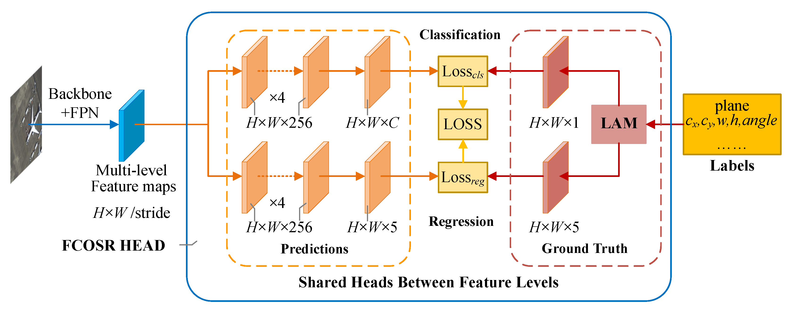
As shown in Figure 1, our method uses the FCOS [11] architecture as a baseline. The network directly predicts the center point (including x and y), width, height, and rotated angle of the target (OpenCV format). We determine the convergence target of the feature map through the LAM. Our algorithm introduces no additional components into the architecture. It removes the center-ness branch [11], which makes the network simpler, with less computation.

Figure 1. FCOSR architecture. The output of the backbone with the feature pyramid network (FPN) [40] is multi-level feature maps, including P3–P7. The head is shared with all multi-level feature maps. The predictions on the left of the head are the inference part, while the other components are only effective during the training stage. The label assignment module (LAM) allocates labels to each feature maps. H and W are the height and width of the feature map, respectively. Stride is the downsampling ratio for multi-level feature maps. C represents the number of categories, and regression branch directly predicts the center point, width, height, and angle of the target.

Figure 1. FCOSR architecture. The output of the backbone with the feature pyramid network (FPN) [40] is multi-level feature maps, including P3–P7. The head is shared with all multi-level feature maps. The predictions on the left of the head are the inference part, while the other components are only effective during the training stage. The label assignment module (LAM) allocates labels to each feature maps. H and W are the height and width of the feature map, respectively. Stride is the downsampling ratio for multi-level feature maps. C represents the number of categories, and regression branch directly predicts the center point, width, height, and angle of the target.

3.1. Network Outputs

The network output contains a C-dimensional vector from the classification branch and a five-dimensional (5D) vector from the regression branch. Unlike FCOS [11], our method aims to give each component of the regression output a different range. The offset can be negative, but the width and height must be positive, and the angle must be limited to 0 to 90 degrees. These simple processes are defined by (1).

$$\begin{array}{cc}\hfill & offse{t}_{xy}=Re{g}_{xy}·k·s\hfill \end{array}$$

(1a)

$$\begin{array}{cc}\hfill & wh=(\mathrm{Elu}(Re{g}_{wh}·k)+1)·s\hfill \end{array}$$

(1b)

$$\begin{array}{cc}\hfill & \theta =\mathrm{Mod}(Re{g}_{\theta },\pi /\phantom{\pi 2}2)\hfill \end{array}$$

(1c)

$Re{g}_{xy}$, $Re{g}_{wh}$, and $Re{g}_{\theta }$ indicate the direct output from the last layer of the regression branch. k is a learnable adjustment factor, and s is the downsampling ratio (stride) for multi-level feature maps. Elu [41] is the improvement of ReLU. Through the calculation of the above equation, the output is converted into a new 5D vector ($offse{t}_x$, $offse{t}_y$, w, h, $angle$). The sampling point coordinates plus offsets are used to obtain target OBBs.

3.2. Ellipse Center Sampling

Center sampling is a strategy used to concentrate sampling points close to the center of the target, which helps reduce low-quality detection and improve model performance. This strategy is used in FCOS [11], YOLOX [3], and other networks, and it consistently improves accuracy. However, there are two problems when directly migrating the horizontal center sampling strategy to oriented object detection. First, the horizontal center sampling area is usually a 3 × 3 or 5 × 5 square [3,11], so the angle of the OBB affects the sampling range. Second, the short edge further reduces the number of sampling points for large-aspect-ratio targets. The most intuitive center sampling is a circular area within a certain range at the center of the target, but the short edge limits the range of center sampling. To mitigate these negative influences, we propose an elliptical center sampling method (ECS) based on 2D Gaussian distribution. Referring to Section 3.2 from ProbIoU [34], we use OBB ($c_x$, $c_y$, w, h, $\theta$) parameters to define a 2D Gaussian distribution [34]:

$$\begin{array}{cc}\hfill & \Sigma =R_{\theta }·{\Sigma }_0·R_{\theta }^T\hfill \end{array}$$

(2a)

$$\begin{array}{cc}\hfill & \mu =(cx,cy)\hfill \end{array}$$

(2b)

$$\begin{array}{cc}\hfill & R_{\theta }=\left[\begin{array}{cc}cos\theta & -sin\theta \\ sin\theta & cos\theta \end{array}\right], {\Sigma }_0=\frac{1}{12}\left[\begin{array}{cc}{w}^2& 0\\ 0& h^2\end{array}\right]\hfill \end{array}$$

(2c)

$\Sigma$ is covariance matrix, ${\Sigma }_0$ is the covariance matrix when the angle is equal to 0, $\mu$ is the mean value, and $R_{\theta }$ is the rotation transformation matrix. Number 12 in (Figure 2c) is a constant obtained by computing the equation for the mean and variance of the Gaussian OBB in ProbIoU (Section 3.2) [34]. The contour of the probability density function of the 2D Gaussian distribution is an elliptical curve. Equation (3) represents the probability density of the 2D Gaussian distribution in the general case.

$$f\left(X\right)=\frac{1}{2\pi {\left|\Sigma \right|}^{1/2}}exp(-\frac{1}{2}{(X-\mu )}^T{\Sigma }^{-1}(X-\mu ))$$

(3)

X indicates the coordinates (2D vector). $\Sigma$ and $\mu$ are same as the related variables in (2). We remove the normalization term from $f\left(X\right)$ and obtain $g\left(X\right)$.

$$g\left(X\right)=exp(-\frac{1}{2}{(X-\mu )}^T{\Sigma }^{-1}(X-\mu ))$$

(4)

$g\left(X\right)\in (0,1]$, which is the elliptic contour of the 2D Gaussian distribution, can be expressed as $g\left(X\right)=C$. When $C=C_0=exp(-1.5)$, the elliptical contour line is just inscribed in the OBB. The range of the elliptic curve expands with the decrease in C, which means that the effective range of C is [$C_0$,1]. Considering that there are many small objects in aerial images, we set C as 0.23 to prevent insufficient sampling caused by a small sampling area. The center sampling area of the target can be determined by $g\left(X\right)\ge C$. If $g\left(X\right)$ is greater than C, the point X is in the sampling area. The elliptical area defined by the target with a large aspect ratio has a slender shape, which puts the part in the long axis direction far away from the center area. In order to solve this problem, we shrink the ellipse sampling region by modifying the Gaussian distribution. We adjusted this (Figure 2c) to define the original covariance matrix in shrinking mode (shrinking elliptical sampling, SES).

$${\Sigma }_0=\frac{min(w,h)}{12}\left[\begin{array}{cc}w& 0\\ 0& h\end{array}\right]$$

(5)

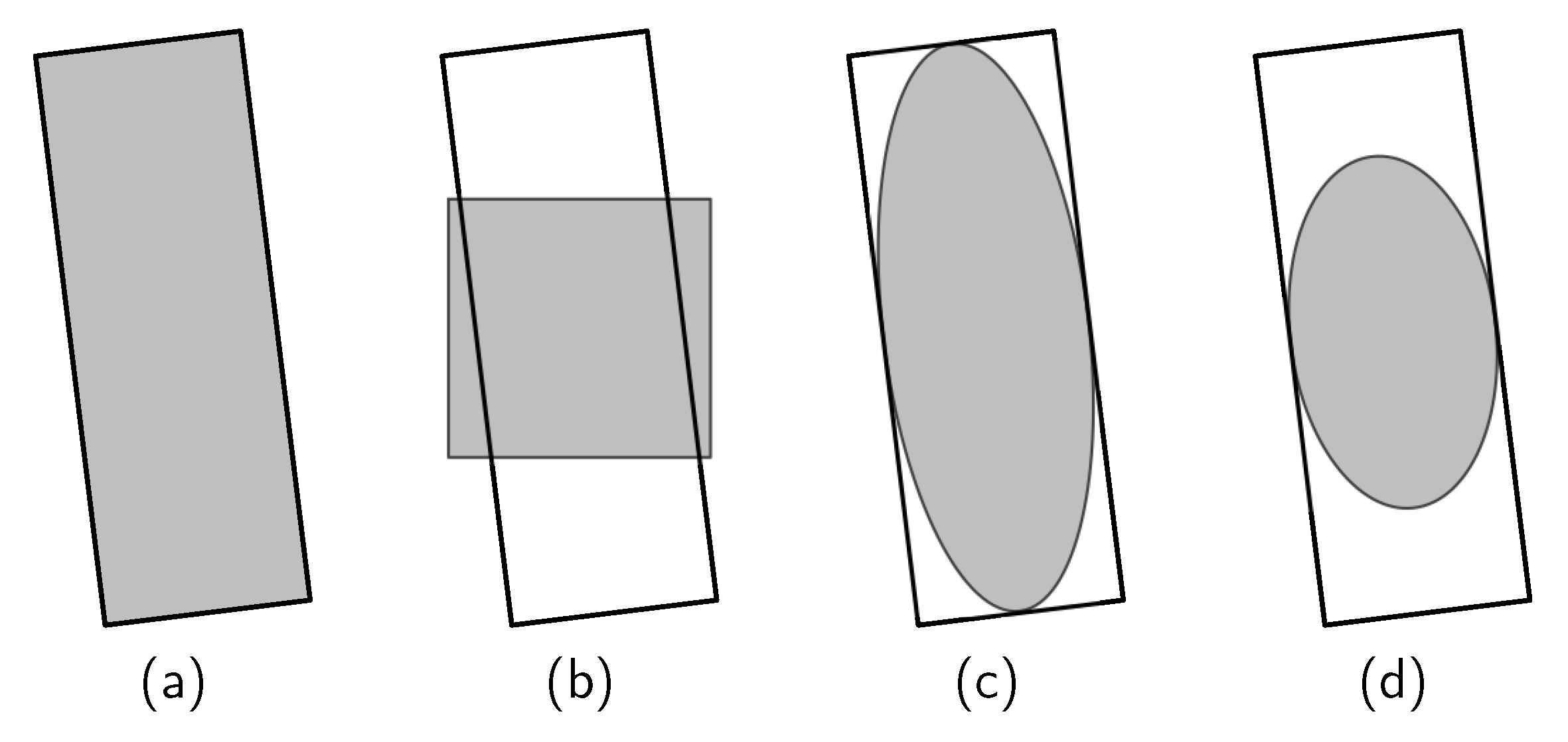
The length of the ellipse major axis shrinks to $\sqrt{wh}$, and that of the minor axis remains unchanged. Figure 2 shows the ellipse center area of OBB. Compared with the horizontal center sampling, the ellipse center sampling is more suitable for OBB, and the sampling area of a large-aspect-ratio target becomes more concentrated by shrinking the long axis.

Figure 2. Ellipse center area of OBB. The oriented rectangle represents the OBB of the target, and the shadow area represents the sampling region: (a) general sampling region, (b) horizontal center sampling region, (c) original elliptical region, and (d) shrinking elliptical region.

Figure 2. Ellipse center area of OBB. The oriented rectangle represents the OBB of the target, and the shadow area represents the sampling region: (a) general sampling region, (b) horizontal center sampling region, (c) original elliptical region, and (d) shrinking elliptical region.

3.3. Fuzzy Sample Label Assignment

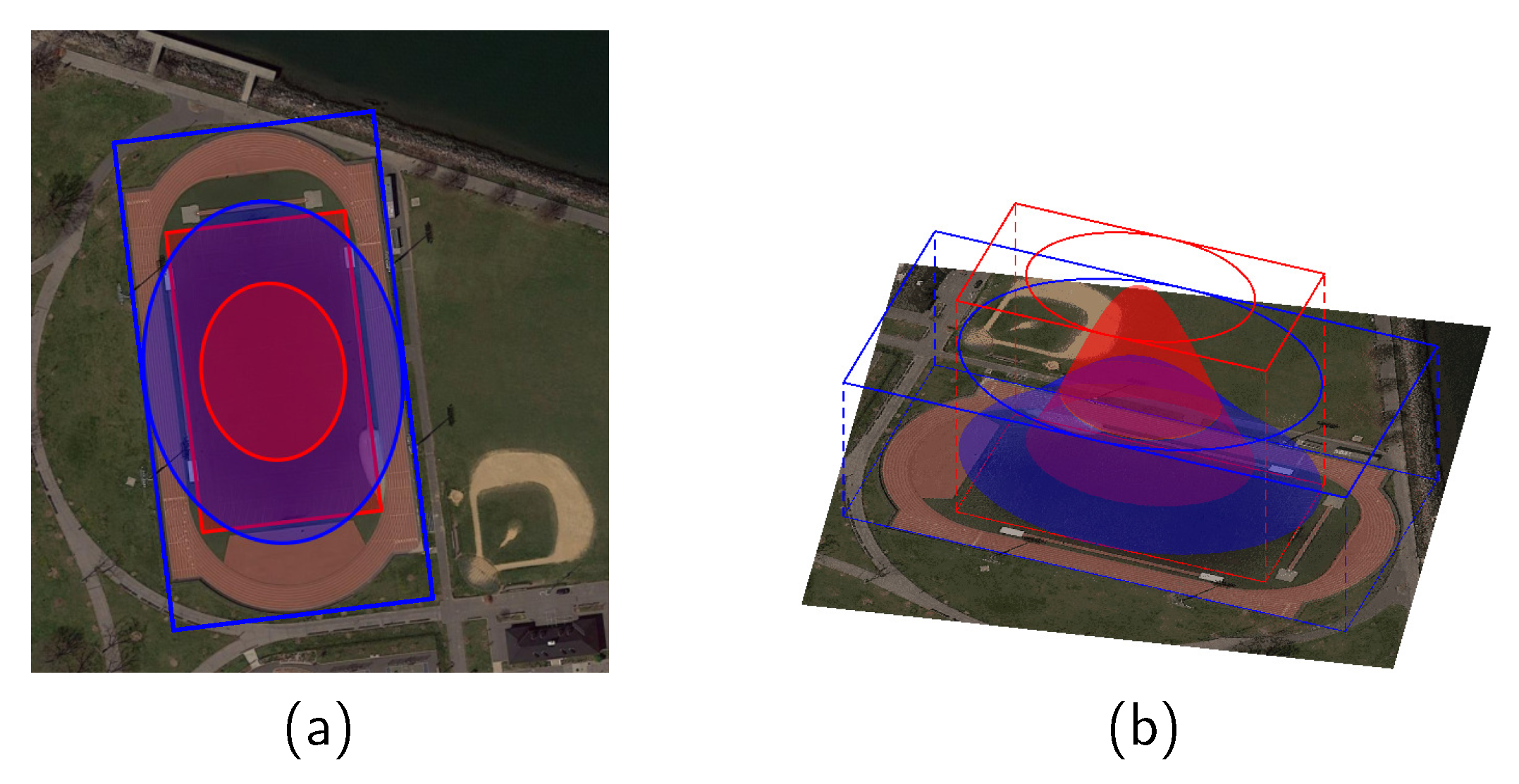
The problem of ambiguous samples arises when the regions of multiple targets overlap. The original FCOS [11] reduces the ambiguous samples by assigning the objects to the specified level of feature maps according to the scale range. For ambiguous samples on the same level of the feature map, FCOS simply represents them by the object with the smallest area. Obviously, this fuzzy sample label assignment method based on the minimum area principle has difficulty dealing with complex scenes, such as aerial scenes. As with the concentric objects in Figure 3, even though the sampling point at the edge of the small object is relatively closer to the center of the large object, FCOS still assigns it to the small object. Intuitively, we decide the attribution of ambiguous samples based on the relative distance between the sampling point and the object centroid. We design a fuzzy sample label assignment method (FLA) to assign ambiguous sample labels based on the 2D Gaussian distribution. The Gaussian distribution has a bell shape, and the response is the largest in its center. The response becomes smaller as the sampling point moves away from the center of the distribution. We approximately take the 2D Gaussian distribution as the distance measure between the sampling point and the object centroid. The center distance is defined by (6).

$$J\left(X\right)=\sqrt{wh}·f\left(X\right)$$

(6)

where $f\left(X\right)$ is the probability density of the 2D Gaussian distribution, which is defined in (3). w and h represent the width and height of the object, respectively. For any object, we calculate the $J\left(X\right)$ value at each sampling point. A larger value of $J\left(X\right)$ means that X is closer to the object. When a sampling point is included by multiple objects at the same time, we assign it to the object with the largest $J\left(X\right)$. Figure 3 shows this fuzzy sample label assignment method more intuitively.

Figure 3. A fuzzy sample label assignment demo: (a) is a 2D label assignment area diagram, and (b) is a 3D visualization effect diagram of $J\left(X\right)$ of two objects. The red OBB and area represent the court object, and the blue represents the ground track field. After $J\left(X\right)$ calculation, smaller areas in the red ellipse are allocated to the court, and other blue areas are allocated to the ground track field.

Figure 3. A fuzzy sample label assignment demo: (a) is a 2D label assignment area diagram, and (b) is a 3D visualization effect diagram of $J\left(X\right)$ of two objects. The red OBB and area represent the court object, and the blue represents the ground track field. After $J\left(X\right)$ calculation, smaller areas in the red ellipse are allocated to the court, and other blue areas are allocated to the ground track field.

3.4. Multi-Level Sampling

The sampling range of the large-aspect-ratio object is mainly affected by the short edge. As shown in Figure 4, when the stride of the feature map is greater than the length of the short edge, the object may be too narrow to be effectively sampled. The higher the level of the feature map, the smaller its size, which means a larger interval between sampling points, and vice versa. However, if the object has a large aspect ratio, there may be only a few, or even zero, sampling points within the object. We thus apply additional sampling to the insufficiently sampled objects. In order to obtain denser sampling points, we need to perform additional sampling on a lower-level feature map. We assign labels to feature maps that satisfy the following two conditions:

$$\begin{array}{cc}\hfill & L_s/Fs<2\hfill \end{array}$$

(7a)

$$\begin{array}{cc}\hfill =& max(W,H)>R_{max}\hfill \end{array}$$

(7b)

where $L_s$ represents the length of the short edge of the object; $Fs$ represents the stride of the feature map; and W and H represent the width and height of minimum bounding rectangle of the OBB, respectively. $R_{max}$ represents the upper limit of the acceptance range of the feature map. The size difference between each level of the feature map is two, so the value of two in the first condition can limit the number of additional samples in our multi-level sampling strategy (MLS). The MLS module extends the sampling region for insufficiently sampled objects. The lower-level feature map represents denser sampling points, which alleviates the insufficient sampling problem.

Figure 4. Multi-level sampling: (a) Insufficient sampling, where green points in the diagram are sampling points. The ship is so narrow that there are no sampling points inside it. (b) A multi-level sampling demo. The red line indicates that the target follows the FCOS guidelines assigned to H6, but it is too narrow to sample effectively. The blue line indicates that the target is assigned to the lower level of features according to the MLS guidelines. This represents the target sampling at three different scales to handle the problem of insufficient sampling.

Figure 4. Multi-level sampling: (a) Insufficient sampling, where green points in the diagram are sampling points. The ship is so narrow that there are no sampling points inside it. (b) A multi-level sampling demo. The red line indicates that the target follows the FCOS guidelines assigned to H6, but it is too narrow to sample effectively. The blue line indicates that the target is assigned to the lower level of features according to the MLS guidelines. This represents the target sampling at three different scales to handle the problem of insufficient sampling.

3.5. Target Loss

The loss of FCOSR consists of classification loss and regression loss. Quality focal loss (QFL) [42] is used for classification loss, which is mainly used to remove the center-ness branch from the original FCOS [11] algorithm. The regression uses the ProbIoU loss [34]. QFL [42] is a part of general focal loss (GFL) [42]. It unifies the training and testing process by replacing the one hot label with the IoU value between the prediction and ground truth. QFL [42] suppresses low-quality detection results and also improves the performance of the model. Equation (8) gives the definition of QFL [42] as

$$QFL\left(\sigma \right)=-{\left|y-\sigma \right|}^{\beta }\left((1-y)log(1-\sigma )+ylog\left(\sigma \right)\right)$$

(8)

where y represents the replaced IoU, and parameter $\beta$ (using the recommend value 2) smoothly controls the down-weighting rate. ProbIoU loss [34] is a type of IoU loss specifically designed for an oriented object. It mainly represents the IoU between OBBs through the distance between 2D Gaussian distributions, which is similar to GWD [32] and KLD [33]. The overall loss can be defined by (9).

$$Loss=\frac{1}{N_{pos}}\sum _{z}QFL+\frac{1}{\sum _z{1}_{\{c_z^{*}>0\}}IoU}·\sum _z{1}_{\{c_z^{*}>0\}}IoU·L\mathrm{os}{\mathrm{s}}_{ProbIoU}$$

(9)

where $N_{pos}$ represents the number of positive samples. The summation is calculated over all locations (z) on the multi-level feature maps. The indicator function is $1_{\{c_z^{*}>0\}}$, being 1 if $c_z^{*}>0$ and 0 otherwise.

4. Experiments

4.1. Datasets

We evaluated our method on the DOTA-v1.0, DOTA-v1.5, and HRSC2016 datasets.

DOTA [21] is a large-scale dataset for aerial object detection. The data are collected from different sensors and platforms. DOTA-v1.0 contains 2806 large aerial images with size ranges from 800 × 800 to 4000 × 4000 and 188,282 instances among 15 common categories: Plane (PL), Baseball diamond (BD), Bridge (BR), Ground track field (GTF), Small vehicle (SV), Large vehicle (LV), Ship (SH), Tennis court (TC), Basketball court (BC), Storage tank (ST), Soccer-ball field (SBF), Roundabout (RA), Harbor (HA), Swimming pool (SP), and Helicopter (HC). DOTA-v1.5 adds the Container Crane (CC) class and instances smaller than 10 pixels on the basis of version 1.0. DOTA-v1.5, which contains 402,089 instances, is more challenging than DOTA-v1.0, but is stable during training. We used both the train and validation sets for training and used the test set for testing. All images were cropped into 1024 × 1024 patches with a gap of 512, and the multi-scale arguments of DOTA-v1.0 were {0.5, 1.0}, while those of DOTA-v1.5 were {0.5, 1.0, 1.5}. We also applied random flipping and the random rotation argument method during training.

HRSC2016 [22] is a challenging ship detection dataset with OBB annotations, which contains 1061 aerial images with a size ranging from 300 × 300 to 1500 × 900. This includes 436, 181, and 444 images in the train, validation and test set, respectively. We used both the train and validation set for training and the test set for testing. All images were resized to 800 × 800 without changing the aspect ratio. Random flipping and random rotation were applied during training.

4.2. Implementation Details

We used ResNext50 [43] with FPN [40] as the backbone for FCOSR and called this model FCOSR-M (medium). We trained the model in 36 epochs for DOTA and 40 k iterations for HRSC2016. We used the SGD optimizer to train the model of DOTA with an initial learning rate (LR) of 0.01, and the LR was divided by 10 at the {24, 33} epoch. The initial LR of the HRSC2016 model was set to 0.001, and the step was {30 k, 36 k} iterations. The momentum and weight decay were 0.9 and 0.0001, respectively. We used the Nvidia DGX Station (4 V100 GPUs@32G, Nvidia, Santa Clara, CA, USA ) with a total batch size of 16 for training, and used a single RTX 2080-Ti GPU, Nvidia, Santa Clara, CA, USA for testing. We adopted Jetson Xavier NX with TensorRT as embedded deployment platforms. The NMS threshold was set to 0.1 when merging image patches, and the confidence threshold was set to 0.1 during testing. Inspired by rotation-equivariant CNNs [20,26], we adopted a new rotation augmentation method, which uses two-step rotation to generate random augmentation data. First, we rotated the image randomly by 0, 90, 180, and 270 degrees with equal probability. Next, we rotated the image randomly by 30 and 60 degrees with 50% probability. Our implementation is based on mmdetection [44].

4.3. Lightweight and Embedded System

We adopted Mobilenet v2 [45] as the backbone, and named it FCOSR-S (small). To deploy FCOSR on the embedded platform, we performed lightweight processing on the model. We adjusted the output stage of the backbone based on FCOSR-S, and replaced the extra convolutional layer of FPN with a pooling layer. We called it FCOSR-lite. On this basis, we further adjusted the feature channel of the head from 256 to 128, and named it FCOSR-tiny. These two models were then converted to the TensorRT 16-bit format and tested on the Nvidia Jetson platform. Figure 5 illustrates a physical picture of the embedded object detection system. As the mainstream oriented object detectors are still designed to run on servers or PCs, we do not have a directly comparable method. Therefore, we compared it with other state-of-the-art (SOTA) methods.

Figure 5. Physical picture of the embedded object detection system based on the Nvidia Jetson platform.

Figure 5. Physical picture of the embedded object detection system based on the Nvidia Jetson platform.

The test was conducted on the DOTA-v1.0 single-scale test set at a 1024 × 1024 image scale. The results are shown in Table 1, and the model size is the TensorRT engine file size (.trt). The FPS denotes the processing number of images by the detector within a one-second interval on Jetson NX and Jetson AGX Xavier devices. The lightweight FCOSR achieved an ideal balance between speed and accuracy on the Jetson device. The lightest tiny model achieved an mAP of 73.93 at 10.68/17.76 FPS. On the Jetson AGX Xavier, it only takes about 2.3 s to process a 5000 × 5000 image. Figure 6 shows the results of the tiny model running on the Jetson AGX Xavier. Our lightweight model quickly and accurately detected densely parked vehicles. This marked a successful attempt to deploy a high-performance oriented object detector on edge computing devices.

Figure 6. The detection result of the entire aerial image on the Nvidia Jetson platform. We completed the detection of P2043 image from the DOTA-v1.0 test set in 1.4 s on a Jetson AGX Xavier device and visualized the results. The size of this large image was 4165 × 3438.

Figure 6. The detection result of the entire aerial image on the Nvidia Jetson platform. We completed the detection of P2043 image from the DOTA-v1.0 test set in 1.4 s on a Jetson AGX Xavier device and visualized the results. The size of this large image was 4165 × 3438.

Table 1. Lightweight FCOSR test results on Jetson platform.

Methods	Parameters	Model Size	Input Size	GFLOPs	FPS	mAP
FCOSR-lite	6.9 M	51.63 MB	1024 × 1024	101.25	7.64/12.59	74.30
FCOSR-tiny	3.52 M	23.2 MB	1024 × 1024	35.89	10.68/17.76	73.93

Table 1. Lightweight FCOSR test results on Jetson platform.

Methods	Parameters	Model Size	Input Size	GFLOPs	FPS	mAP
FCOSR-lite	6.9 M	51.63 MB	1024 × 1024	101.25	7.64/12.59	74.30
FCOSR-tiny	3.52 M	23.2 MB	1024 × 1024	35.89	10.68/17.76	73.93

4.4. Comparison with State-of-the-Art Methods

We used a variety of other backbones to replace ResNext50 [43] to reconstruct the FCOSR model. We tested FCOSR on ResNext101 [43] with 64 groups and 4 widths, and named this model FCOSR-L (large). The parameters, input patch size, FLOPs, FPS, and mAP on DOTA are shown in Table 2. FPS represents the result tested on a single RTX 2080-Ti device. mAP is the result on DOTA-v1.0 with single-scale evaluation.

Table 2. FCOSR series model size, FLOPs, FPS, and mAP comparison.

Method	Backbone	Parameters	Input Size	GFLOPs	FPS	mAP
FCOSR-S	Mobilenet v2	7.32 M	1024 × 1024	101.42	23.7	74.05
FCOSR-M	ResNext50	31.4 M	1024 × 1024	210.01	14.6	77.15
FCOSR-L	ResNext101	89.64 M	1024 × 1024	445.75	7.9	77.39

Table 2. FCOSR series model size, FLOPs, FPS, and mAP comparison.

Method	Backbone	Parameters	Input Size	GFLOPs	FPS	mAP
FCOSR-S	Mobilenet v2	7.32 M	1024 × 1024	101.42	23.7	74.05
FCOSR-M	ResNext50	31.4 M	1024 × 1024	210.01	14.6	77.15
FCOSR-L	ResNext101	89.64 M	1024 × 1024	445.75	7.9	77.39

Results on DOTA-v1.0: As shown in Table 3, we compared the FCOSR series with other SOTA methods on the DOTA-v1.0 OBB task. ROI-Trans. and BBAVec. indicate ROI-transformer and BBAVectors, respectively; R, RX, ReR, H, and Mobile indicate ResNet, ResNext, ReResNet, Hourglass, and MoblieNet v2, respectively; * indicates multi-scale training and testing. The results in red and blue indicate the best and second-best results in each column, respectively.

Our method enables a significant performance improvement over other anchor-based methods at the same model scale, namely ROI-transformer [15], CenterMap [46], SCRDet++ [47], R${}^3$Det [28], and CSL [29]. It is only outperformed by S${}^2$ANet [16] and ReDet [20] in the multi-scale training and testing, while our medium and large models are more accurate than other methods in the single-scale evaluation.

Compared with other anchor-free methods, FCOSR-M achieved an mAP of 79.25 under multi-scale training and testing, and achieved the best or second-best accuracy in nine subcategories. Our small model showed competitive performance at multiple scales, and its accuracy was at the same level as that of most models. However, it is much smaller than other models and therefore faster. The results in Section 4.6 also support this view.

We also note that FCOSR-L performed worse than the medium model at multiple scales, and the performance improvement at a single scale was small. From Table 3, we can see that the performance improvement brought by ResNext101 was much smaller than that of other methods, but when tuning from the ResNext50 to Mobilenet backbone, FCOSR-S outperformed the other methods in both speed and accuracy. Therefore, we believe that the FCOSR series rapidly reaches peak performance as the trunk size increases, and is more suitable for small- and medium-sized models. From the overall results shown in Table 3, although there is still a clear gap in speed and accuracy compared with the anchor-based model, our algorithm achieved better performance than other anchor-free methods. We visualized a part of the DOTA-v1.0 test set result in Figure 7. The detection domain of our model covers various scales of targets, and it works well for dense vehicles in parking lots, stadiums, and runways (area overlap).

Results on DOTA-v1.5: As shown in Table 4, we also conducted all experiments on the FCOSR series. RN-O., FR-O., and MR. indicate Retinanet-oriented, Faster-RCNN-oriented, and Mask RCNN, respectively; † and ‡ refer to one-stage and two-stage anchor-based methods, respectively; and * indicates multi-scale training and testing. There are currently only a few methods for evaluating the DOTA-v1.5 dataset, so we directly used some results in ReDet [20] and the RotationDetection repository (https://github.com/yangxue0827/RotationDetection (accessed on 1 August 2023)).

Table 3. Comparison with state-of-the-art methods on the DOTA-v1.0 OBB task.

Method	Backbone	PL	BD	BR	GTF	SV	LV	SH	TC	BC	ST	SBF	RA	HA	SP	HC	mAP
Anchor-based, two-stage
ROI-Trans. * [15]	R101	88.64	78.52	43.44	75.92	68.81	73.68	83.59	90.74	77.27	81.46	58.39	53.54	62.83	58.93	47.67	69.56
CenterMap * [46]	R101	89.83	84.41	54.60	70.25	77.66	78.32	87.19	90.66	84.89	85.27	56.46	69.23	74.13	71.56	66.06	76.03
SCRDet++ * [47]	R101	90.05	84.39	55.44	73.99	77.54	71.11	86.05	90.67	87.32	87.08	69.62	68.90	73.74	71.29	65.08	76.81
ReDet [20]	ReR50	88.79	82.64	53.97	74.00	78.13	84.06	88.04	90.89	87.78	85.75	61.76	60.39	75.96	68.07	63.59	76.25
ReDet * [20]	ReR50	88.81	82.48	60.83	80.82	78.34	86.06	88.31	90.87	88.77	87.03	68.65	66.90	79.26	79.71	74.67	80.10
Anchor-based, one-stage
R${}^3$Det * [28]	R152	89.80	83.77	48.11	66.77	78.76	83.27	87.84	90.82	85.38	85.51	65.67	62.68	67.53	78.56	72.62	76.47
CSL * [29]	R152	90.13	84.43	54.57	68.13	77.32	72.98	85.94	90.74	85.95	86.36	63.42	65.82	74.06	73.67	70.08	76.24
S${}^2$ANet * [16]	R50	89.11	82.84	48.37	71.11	78.11	78.39	87.25	90.83	84.90	85.64	60.36	62.60	65.26	69.13	57.94	74.12
S${}^2$ANet * [16]	R50	88.89	83.60	57.74	81.95	79.94	83.19	89.11	90.78	84.87	87.81	70.30	68.25	78.30	77.01	69.58	79.42
Anchor-free, one-stage
BBAVec. * [17]	R101	88.63	84.06	52.13	69.56	78.26	80.40	88.06	90.87	87.23	86.39	56.11	65.62	67.10	72.08	63.96	75.36
DRN * [48]	H104	89.45	83.16	48.98	62.24	70.63	74.25	83.99	90.73	84.60	85.35	55.76	60.79	71.56	68.82	63.92	72.95
CFA [49]	R101	89.26	81.72	51.81	67.17	79.99	78.25	84.46	90.77	83.40	85.54	54.86	67.75	73.04	70.24	64.96	75.05
PolarDet [18]	R50	89.73	87.05	45.30	63.32	78.44	76.65	87.13	90.79	80.58	85.89	60.97	67.94	68.20	74.63	68.67	75.02
PolarDet * [18]	R101	89.65	87.07	48.14	70.97	78.53	80.34	87.45	90.76	85.63	86.87	61.64	70.32	71.92	73.09	67.15	76.64
FCOSR-S	Mobile	89.09	80.58	44.04	73.33	79.07	76.54	87.28	90.88	84.89	85.37	55.95	64.56	66.92	76.96	55.32	74.05
FCOSR-S *	Mobile	88.60	84.13	46.85	78.22	79.51	77.00	87.74	90.85	86.84	86.71	64.51	68.17	67.87	72.08	62.52	76.11
FCOSR-M	RX50	88.88	82.68	50.10	71.34	81.09	77.40	88.32	90.80	86.03	85.23	61.32	68.07	75.19	80.37	70.48	77.15
FCOSR-M *	RX50	89.06	84.93	52.81	76.32	81.54	81.81	88.27	90.86	85.20	87.58	68.63	70.38	75.95	79.73	75.67	79.25
FCOSR-L	RX101	89.50	84.42	52.58	71.81	80.49	77.72	88.23	90.84	84.23	86.48	61.21	67.77	76.34	74.39	74.86	77.39
FCOSR-L *	RX101	88.78	85.38	54.29	76.81	81.52	82.76	88.38	90.80	86.61	87.25	67.58	67.03	76.86	73.22	74.68	78.80

Table 3. Comparison with state-of-the-art methods on the DOTA-v1.0 OBB task.

Method	Backbone	PL	BD	BR	GTF	SV	LV	SH	TC	BC	ST	SBF	RA	HA	SP	HC	mAP
Anchor-based, two-stage
ROI-Trans. * [15]	R101	88.64	78.52	43.44	75.92	68.81	73.68	83.59	90.74	77.27	81.46	58.39	53.54	62.83	58.93	47.67	69.56
CenterMap * [46]	R101	89.83	84.41	54.60	70.25	77.66	78.32	87.19	90.66	84.89	85.27	56.46	69.23	74.13	71.56	66.06	76.03
SCRDet++ * [47]	R101	90.05	84.39	55.44	73.99	77.54	71.11	86.05	90.67	87.32	87.08	69.62	68.90	73.74	71.29	65.08	76.81
ReDet [20]	ReR50	88.79	82.64	53.97	74.00	78.13	84.06	88.04	90.89	87.78	85.75	61.76	60.39	75.96	68.07	63.59	76.25
ReDet * [20]	ReR50	88.81	82.48	60.83	80.82	78.34	86.06	88.31	90.87	88.77	87.03	68.65	66.90	79.26	79.71	74.67	80.10
Anchor-based, one-stage
R${}^3$Det * [28]	R152	89.80	83.77	48.11	66.77	78.76	83.27	87.84	90.82	85.38	85.51	65.67	62.68	67.53	78.56	72.62	76.47
CSL * [29]	R152	90.13	84.43	54.57	68.13	77.32	72.98	85.94	90.74	85.95	86.36	63.42	65.82	74.06	73.67	70.08	76.24
S${}^2$ANet * [16]	R50	89.11	82.84	48.37	71.11	78.11	78.39	87.25	90.83	84.90	85.64	60.36	62.60	65.26	69.13	57.94	74.12
S${}^2$ANet * [16]	R50	88.89	83.60	57.74	81.95	79.94	83.19	89.11	90.78	84.87	87.81	70.30	68.25	78.30	77.01	69.58	79.42
Anchor-free, one-stage
BBAVec. * [17]	R101	88.63	84.06	52.13	69.56	78.26	80.40	88.06	90.87	87.23	86.39	56.11	65.62	67.10	72.08	63.96	75.36
DRN * [48]	H104	89.45	83.16	48.98	62.24	70.63	74.25	83.99	90.73	84.60	85.35	55.76	60.79	71.56	68.82	63.92	72.95
CFA [49]	R101	89.26	81.72	51.81	67.17	79.99	78.25	84.46	90.77	83.40	85.54	54.86	67.75	73.04	70.24	64.96	75.05
PolarDet [18]	R50	89.73	87.05	45.30	63.32	78.44	76.65	87.13	90.79	80.58	85.89	60.97	67.94	68.20	74.63	68.67	75.02
PolarDet * [18]	R101	89.65	87.07	48.14	70.97	78.53	80.34	87.45	90.76	85.63	86.87	61.64	70.32	71.92	73.09	67.15	76.64
FCOSR-S	Mobile	89.09	80.58	44.04	73.33	79.07	76.54	87.28	90.88	84.89	85.37	55.95	64.56	66.92	76.96	55.32	74.05
FCOSR-S *	Mobile	88.60	84.13	46.85	78.22	79.51	77.00	87.74	90.85	86.84	86.71	64.51	68.17	67.87	72.08	62.52	76.11
FCOSR-M	RX50	88.88	82.68	50.10	71.34	81.09	77.40	88.32	90.80	86.03	85.23	61.32	68.07	75.19	80.37	70.48	77.15
FCOSR-M *	RX50	89.06	84.93	52.81	76.32	81.54	81.81	88.27	90.86	85.20	87.58	68.63	70.38	75.95	79.73	75.67	79.25
FCOSR-L	RX101	89.50	84.42	52.58	71.81	80.49	77.72	88.23	90.84	84.23	86.48	61.21	67.77	76.34	74.39	74.86	77.39
FCOSR-L *	RX101	88.78	85.38	54.29	76.81	81.52	82.76	88.38	90.80	86.61	87.25	67.58	67.03	76.86	73.22	74.68	78.80

Table 4. Comparison with state-of-the-art methods on the DOTA-v1.5 OBB task.

Method	Backbone	PL	BD	BR	GTF	SV	LV	SH	TC	BC	ST	SBF	RA	HA	SP	HC	CC	mAP
RN-O. † [10]	R50	71.43	77.64	42.12	64.65	44.53	56.79	73.31	90.84	76.02	59.96	46.95	69.24	59.65	64.52	48.06	0.83	59.16
FR-O. ‡ [8]	R50	71.89	74.47	44.45	59.87	51.28	68.98	79.37	90.78	77.38	67.50	47.75	69.72	61.22	65.28	60.47	1.54	62.00
MR. ‡ [9]	R50	76.84	73.51	49.90	57.80	51.31	71.34	79.75	90.46	74.21	66.07	46.21	70.61	63.07	64.46	57.81	9.42	62.67
DAFNe * [50]	R101	80.69	86.38	52.14	62.88	67.03	76.71	88.99	90.84	77.29	83.41	51.74	74.60	75.98	75.78	72.46	34.84	71.99
FCOS [11]	R50	78.67	72.50	44.31	59.57	56.25	64.03	78.06	89.40	71.45	73.32	49.51	66.47	55.78	63.26	44.76	9.44	61.05
ReDet ‡ [20]	ReR50	79.20	82.81	51.92	71.41	52.38	75.73	80.92	90.83	75.81	68.64	49.29	72.03	73.36	70.55	63.33	11.53	66.86
ReDet $‡*$ [20]	ReR50	88.51	86.45	61.23	81.20	67.60	83.65	90.00	90.86	84.30	75.33	71.49	72.06	78.32	74.73	76.10	46.98	76.80
FCOSR-S	Mobile	80.05	76.98	44.49	74.17	51.09	74.07	80.60	90.87	78.40	75.01	53.38	69.35	66.33	74.43	59.22	13.50	66.37
FCOSR-S *	Mobile	87.84	84.60	53.35	75.67	65.79	80.71	89.30	90.89	84.18	84.23	63.53	73.07	73.29	76.15	72.64	14.72	73.12
FCOSR-M	RX50	80.48	81.90	50.02	72.32	56.82	76.37	81.06	90.86	78.62	77.32	53.63	66.92	73.78	74.20	69.80	15.73	68.74
FCOSR-M *	RX50	80.85	83.89	53.36	76.24	66.85	82.54	89.61	90.87	80.11	84.27	61.72	72.90	76.23	75.28	70.01	35.87	73.79
FCOSR-L	RX101	80.58	85.25	51.05	70.83	57.77	76.72	81.09	90.87	78.07	77.60	51.91	68.72	75.87	72.61	69.30	31.06	69.96
FCOSR-L *	RX101	87.12	83.90	53.41	70.99	66.79	82.84	89.66	90.85	81.84	84.52	67.78	74.52	77.25	74.97	75.31	44.81	75.41

Table 4. Comparison with state-of-the-art methods on the DOTA-v1.5 OBB task.

Method	Backbone	PL	BD	BR	GTF	SV	LV	SH	TC	BC	ST	SBF	RA	HA	SP	HC	CC	mAP
RN-O. † [10]	R50	71.43	77.64	42.12	64.65	44.53	56.79	73.31	90.84	76.02	59.96	46.95	69.24	59.65	64.52	48.06	0.83	59.16
FR-O. ‡ [8]	R50	71.89	74.47	44.45	59.87	51.28	68.98	79.37	90.78	77.38	67.50	47.75	69.72	61.22	65.28	60.47	1.54	62.00
MR. ‡ [9]	R50	76.84	73.51	49.90	57.80	51.31	71.34	79.75	90.46	74.21	66.07	46.21	70.61	63.07	64.46	57.81	9.42	62.67
DAFNe * [50]	R101	80.69	86.38	52.14	62.88	67.03	76.71	88.99	90.84	77.29	83.41	51.74	74.60	75.98	75.78	72.46	34.84	71.99
FCOS [11]	R50	78.67	72.50	44.31	59.57	56.25	64.03	78.06	89.40	71.45	73.32	49.51	66.47	55.78	63.26	44.76	9.44	61.05
ReDet ‡ [20]	ReR50	79.20	82.81	51.92	71.41	52.38	75.73	80.92	90.83	75.81	68.64	49.29	72.03	73.36	70.55	63.33	11.53	66.86
ReDet $‡*$ [20]	ReR50	88.51	86.45	61.23	81.20	67.60	83.65	90.00	90.86	84.30	75.33	71.49	72.06	78.32	74.73	76.10	46.98	76.80
FCOSR-S	Mobile	80.05	76.98	44.49	74.17	51.09	74.07	80.60	90.87	78.40	75.01	53.38	69.35	66.33	74.43	59.22	13.50	66.37
FCOSR-S *	Mobile	87.84	84.60	53.35	75.67	65.79	80.71	89.30	90.89	84.18	84.23	63.53	73.07	73.29	76.15	72.64	14.72	73.12
FCOSR-M	RX50	80.48	81.90	50.02	72.32	56.82	76.37	81.06	90.86	78.62	77.32	53.63	66.92	73.78	74.20	69.80	15.73	68.74
FCOSR-M *	RX50	80.85	83.89	53.36	76.24	66.85	82.54	89.61	90.87	80.11	84.27	61.72	72.90	76.23	75.28	70.01	35.87	73.79
FCOSR-L	RX101	80.58	85.25	51.05	70.83	57.77	76.72	81.09	90.87	78.07	77.60	51.91	68.72	75.87	72.61	69.30	31.06	69.96
FCOSR-L *	RX101	87.12	83.90	53.41	70.99	66.79	82.84	89.66	90.85	81.84	84.52	67.78	74.52	77.25	74.97	75.31	44.81	75.41

Figure 7. The FCOSR-M detection result on the DOTA-v1.0 test set. The confidence threshold is set to 0.3 when showing these results.

Figure 7. The FCOSR-M detection result on the DOTA-v1.0 test set. The confidence threshold is set to 0.3 when showing these results.

From a single-scale perspective, the medium-sized and large models achieved mAP values of 68.74 and 69.96, respectively, which were much higher than the results for other models. The small model achieved an mAP of 66.37, slightly lower than ReDet’s 66.86 mAP, while the Mobilenet v2 backbone used by the small model made it much faster than the other methods. As DOTA-v1.5 is only generated by adding a new category to version 1.0, the actual inference speed of the model was close to that of version 1.0. Referring to the results in Section 4.6, we can see that the inference speed of the small model is 23.7 FPS at this time, while the speed of ReDet is only 8.8 FPS, and the medium-sized model of the same scale maintains 14.6 FPS.

Classical object detection algorithms such as Faster-RCNN-O can maintain the same speed as FCOSR, but with much less accuracy. Compared with the original FCOS model, our method has a redesigned label assignment strategy for the characteristics of aerial images, which is more suitable for oriented target detection. Our method maintains competitive results at multiple scales. Although the performance is still lower than that of two-stage anchor-based methods such as ReDet, our method shrinks the huge gap in performance between anchor-free and anchor-based methods.

Results on HRSC2016: We compared our method with other one-stage methods. We repeated the experiment 10 times and recorded the mean and standard deviation in Table 5. FCOSR series models surpassed all anchor-free models and achieved an mAP of 95.70 under the VOC2012 metrics. FCOSR series models exceeded an mAP of 90 under the VOC2007 metrics. The large one even surpassed S${}^2$ANet [16], which further proves that our proposed anchor-free method has a performance equivalent to that of the anchor-based method. The detection results are shown in Figure 8. In complex background environments, our model accurately detected various scales of ship targets. The model displayed good detection of slender ships docked in ports, as well as ships in shipyards.

Table 5. Comparison with state-of-the-art methods on HRSC2016.

Method	Backbone	mAP (07)	mAP (12)
PIoU [19]	DLA-34	89.20	-
S${}^2$ANet [16]	ResNet101	90.17	95.01
ProbIoU [34]	ResNet50	87.09	-
DRN [48]	Hourglass104	-	92.70
CenterMap [46]	ResNet50	-	92.80
BBAVectors [17]	ResNet101	88.60	-
PolarDet [18]	ResNet50	90.13	-
FCOSR-S(ours)	Mobilenet v2	90.05 (±0.042)	92.59 (±0.054)
FCOSR-M(ours)	ResNext50	90.12 (±0.034)	94.81 (±0.030)
FCOSR-L(ours)	ResNext101	90.13 (±0.028)	95.70 (±0.026)

Table 5. Comparison with state-of-the-art methods on HRSC2016.

Method	Backbone	mAP (07)	mAP (12)
PIoU [19]	DLA-34	89.20	-
S${}^2$ANet [16]	ResNet101	90.17	95.01
ProbIoU [34]	ResNet50	87.09	-
DRN [48]	Hourglass104	-	92.70
CenterMap [46]	ResNet50	-	92.80
BBAVectors [17]	ResNet101	88.60	-
PolarDet [18]	ResNet50	90.13	-
FCOSR-S(ours)	Mobilenet v2	90.05 (±0.042)	92.59 (±0.054)
FCOSR-M(ours)	ResNext50	90.12 (±0.034)	94.81 (±0.030)
FCOSR-L(ours)	ResNext101	90.13 (±0.028)	95.70 (±0.026)

Figure 8. The FCOSR-L detection result on HRSC2016. The confidence threshold is set to 0.3 when visualizing these results.

Figure 8. The FCOSR-L detection result on HRSC2016. The confidence threshold is set to 0.3 when visualizing these results.

4.5. Ablation Experiments

We performed a series of experiments on the DOTA-v1.0 test set to evaluate the effectiveness of the proposed method. We used FCOSR-M (medium) as the baseline. We trained and tested the model at a single scale.

As shown in Table 6, the mAP at the baseline for FCOS-M is 70.4, which increases by 4.03 with the addition of rotation augmentation. When QFL [42] was used instead of focal loss, the detection result of the model gained an mAP of 0.91. Next, we tried to add ECS, FLA, and MLS modules and when used individually, the results were improved by 1.03, 0.58, and 0.34, respectively. Applying ECS and FLA at the same time, the detection result was improved to 76.80. Using all the modules brought the result up to 77.15. Through the use of multiple modules, FCOSR-M achieved a significant performance improvement over anchor-based methods. These modules do not have any additional calculations when making inferences, which makes FCOSR a simple, fast, and easy-to-deploy OBB detector.

Table 6. Results of ablation experiments for FCOSR-M on single scale.

Method	Rotate Aug.	QFL	ECS	FLA	MLS	mAP
						70.40
	✓					74.43
FCOSR-M	✓	✓				75.34
	✓	✓	✓			76.37
	✓	✓		✓		75.92
	✓	✓			✓	75.77
	✓	✓	✓	✓		76.80
	✓	✓	✓	✓	✓	77.15

Table 6. Results of ablation experiments for FCOSR-M on single scale.

Method	Rotate Aug.	QFL	ECS	FLA	MLS	mAP
						70.40
	✓					74.43
FCOSR-M	✓	✓				75.34
	✓	✓	✓			76.37
	✓	✓		✓		75.92
	✓	✓			✓	75.77
	✓	✓	✓	✓		76.80
	✓	✓	✓	✓	✓	77.15

Effectiveness of ellipse center sampling: We changed the sampling regions of the FCOSR-M baseline to the shapes listed in Figure 2. Table 7 shows the results of the comparison experiments. The general sampling region (GS), horizontal center sampling region (HCS), and original elliptical sampling region (OES) achieved mAPs of 76.34, 75.48, and 76.70, respectively. These results are all lower than those of the standard FCOSR-M model. The HCS strategy is widely used in HBB detection. However, an OBB carries a rotation angle, so the horizontal fixed-scale sampling area does not match it effectively, further decreasing the number of positive samples. This makes the baseline performance of FCOSR with the HCS strategy lower than that of other strategies. The edge region of the OBB of many aerial targets is part of the background, such as aircraft, ships, and other targets. Directly applying the GS strategy tends to lead to incorrectly sampling the actual background area as a positive sample. The ellipse center sampling scheme removes part of the edge regions of the OBB. This effect is further enhanced by shrinking the long axis of the ellipse so that the SES-based FCOSR baseline has better overall performance. The difference between SES and HCS is that SES is not a fixed-scale sampling strategy, but calculates the range by using a 2D Gaussian function. Therefore, SES has the advantage of converting the Euclidean distance to Gaussian distance so that we can easily obtain an elliptical region matching the OBB.

The results for the elliptical shape sampling region are better than those of other schemes. The FCOSR based on the shrinking ellipse center sampling achieved an mAP of 77.15, demonstrating performance that is equivalent to that of other mainstream state-of-the-art models. The above experimental results validate the effectiveness of our proposed method.

Table 7. Results of experiments comparing the different sampling ranges listed in Figure 2.

Method	PL	BD	BR	GTF	SV	LV	SH	TC	BC	ST	SBF	RA	HA	SP	HC	mAP
GS	89.40	83.73	50.97	71.42	80.87	77.81	88.49	90.76	85.36	85.45	60.12	62.98	76.22	75.64	65.93	76.34
HCS	88.09	79.57	55.31	63.63	81.13	77.67	88.11	90.80	84.85	84.11	58.75	62.29	74.29	80.51	63.11	75.48
OES	89.07	81.15	50.96	70.44	80.53	77.64	88.31	90.85	85.37	86.60	59.05	61.22	76.00	80.58	72.73	76.70
SES	88.88	82.68	50.10	71.34	81.09	77.40	88.32	90.80	86.03	85.23	61.32	68.07	75.19	80.37	70.48	77.15

Table 7. Results of experiments comparing the different sampling ranges listed in Figure 2.

Method	PL	BD	BR	GTF	SV	LV	SH	TC	BC	ST	SBF	RA	HA	SP	HC	mAP
GS	89.40	83.73	50.97	71.42	80.87	77.81	88.49	90.76	85.36	85.45	60.12	62.98	76.22	75.64	65.93	76.34
HCS	88.09	79.57	55.31	63.63	81.13	77.67	88.11	90.80	84.85	84.11	58.75	62.29	74.29	80.51	63.11	75.48
OES	89.07	81.15	50.96	70.44	80.53	77.64	88.31	90.85	85.37	86.60	59.05	61.22	76.00	80.58	72.73	76.70
SES	88.88	82.68	50.10	71.34	81.09	77.40	88.32	90.80	86.03	85.23	61.32	68.07	75.19	80.37	70.48	77.15

Effectiveness of fuzzy sample label assignment: We used FCOSR-M as the baseline. Training and testing was performed on DOTA-v1.0, and all parts were unchanged except the label assignment method (LAM). We replaced our LAM with ATSS [51] and simOTA [3], and Table 8 shows the results of the comparison experiments. ATSS [51] and simOTA [3] achieve an mAP of 76.60 and 72.63, respectively, both of which are lower than our reported mAP of 77.15. simOTA [3] achieves strong results in the HBB object detection task, but the experimental results show that it may not be suitable for OBB object detection. Oriented objects have more difficulty converging than horizontal objects. Therefore, a small number of samples were actually used for the training, which directly affected the performance of the model. ATSS [51] is designed based on the central sampling principle, which is similar to our method. However, both ATSS and simOTA are designed based on natural scenes, which do not match with the characteristics of remote sensing image objects. As a result, the actual effect is not as good as that of our proposed method.

Table 8. Results of experiments comparing label assignment methods.

Method	PL	BD	BR	GTF	SV	LV	SH	TC	BC	ST	SBF	RA	HA	SP	HC	mAP
ATSS [51]	88.91	81.79	53.93	72.42	80.75	80.77	88.33	90.79	86.27	85.54	56.99	63.19	75.90	74.61	68.87	76.60
simOTA [3]	81.31	72.89	52.85	69.79	79.89	77.17	86.87	90.11	83.07	82.38	58.96	58.31	74.37	68.75	52.74	72.63
Ours	88.88	82.68	50.10	71.34	81.09	77.40	88.32	90.80	86.03	85.23	61.32	68.07	75.19	80.37	70.48	77.15

Table 8. Results of experiments comparing label assignment methods.

Method	PL	BD	BR	GTF	SV	LV	SH	TC	BC	ST	SBF	RA	HA	SP	HC	mAP
ATSS [51]	88.91	81.79	53.93	72.42	80.75	80.77	88.33	90.79	86.27	85.54	56.99	63.19	75.90	74.61	68.87	76.60
simOTA [3]	81.31	72.89	52.85	69.79	79.89	77.17	86.87	90.11	83.07	82.38	58.96	58.31	74.37	68.75	52.74	72.63
Ours	88.88	82.68	50.10	71.34	81.09	77.40	88.32	90.80	86.03	85.23	61.32	68.07	75.19	80.37	70.48	77.15

Effectiveness of multi-level sampling: As shown in Table 6, the addition of the MLS module brings a 0.35–0.43 improvement in mAP. Targets in aerial image scenes are oriented arbitrarily, and there are many slender targets. This causes insufficient sampling of the target, which affects the performance for that type of target. The MLS module solves this problem by extending the sampling region for insufficiently sampled objects. Experimental results validate the effectiveness of the MLS method.

4.6. Speed versus Accuracy

We tested the inference speed of FCOSR series models and other open-source mainstream models, including R${}^3$Det [28], ReDet [20], S${}^2$ANet [16], Faster-RCNN-O (FR-O) [8], Oriented RCNN (O-RCNN) [27], and RetinaNet-O (RN-O) [10]. For convenience, we tested Faster-RCNN-O [8] and RetinaNet-O models in the Oriented-RCNN repository (https://github.com/jbwang1997/OBBDetection (accessed on 1 August 2023)). All tests were conducted on a single RTX 2080-Ti device at a 1024 × 1024 image scale.

The test results are shown in Figure 9. The accuracy of all models increased as the number of model parameters increased. FCOSR’s medium-sized and small models both outperformed other anchor-based methods with the same backbone size. FCOSR-M exceeded almost the same speed S${}^2$ANet [16] and Oriented RCNN [27] 3.03 mAP and 1.28 mAP, respectively. This is because of the simple and lightweight head structure and the well-designed label assignment strategy. FCOSR-S even achieved an mAP of 74.05 at a speed of 23.7 FPS, making it the fastest high-performance model currently. The FCOSR series models surpassed the existing mainstream models in speed and accuracy, which also proves that, through reasonable label assignment, even a simple model can achieve excellent performance.

Figure 9. Speed versus accuracy on DOTA-v1.0 single-scale test set. X indicates the ResNext backbone. R indicates the ResNet backbone. RR indicates the ReResNet(ReDet) backbone. Mobile indicates the Mobilenet v2 backbone. We tested ReDet [20], S${}^2$ANet [16], and R${}^3$Det [28] on a single RTX 2080-Ti device based on their source code. Faster-RCNN-O (FR-O) [8], RetinaNet-O (RN-O) [10], and Oriented RCNN (O-RCNN) [27] test results are from the OBBDetection repository².

Figure 9. Speed versus accuracy on DOTA-v1.0 single-scale test set. X indicates the ResNext backbone. R indicates the ResNet backbone. RR indicates the ReResNet(ReDet) backbone. Mobile indicates the Mobilenet v2 backbone. We tested ReDet [20], S${}^2$ANet [16], and R${}^3$Det [28] on a single RTX 2080-Ti device based on their source code. Faster-RCNN-O (FR-O) [8], RetinaNet-O (RN-O) [10], and Oriented RCNN (O-RCNN) [27] test results are from the OBBDetection repository².

5. Conclusions

Anchor-based oriented detectors require manual preset boxes, which introduce additional hyper-parameters and calculations. They often use more complex architectures for better performance; this makes them difficult to deploy on embedded platforms. To make deployment easier, we take FCOS as a baseline and propose a novel label assignment strategy to allocate more reasonable labels to the samples. The proposed method is improved for the features of aerial image objects. The label assignment strategy consists of three parts: ellipse center sampling, fuzzy sample label assignment, and multi-level sampling. Compared to the original FCOS label assignment strategy, our method produces more reasonable matches. Thus, the model achieves better performance. Due to its simple architecture, FCOSR does not have any special computing units for inferencing. Therefore, it is a fast and easy-to-deploy model on most platforms. Our experiments on a lightweight backbone also demonstrate satisfactory results. The results of extensive experiments on the DOTA and HRSC2016 datasets demonstrate the effectiveness of our method.

References

- Redmon, J.; Divvala, S.; Girshick, R.; Farhadi, A. You only look once: Unified, real-time object detection. In Proceedings of the IEEE Conference on Computer Vision and Pattern Recognition, Las Vegas, NV, USA, 26 June–1 July 2016; pp. 779–788. [Google Scholar]
- Redmon, J.; Farhadi, A. Yolov3: An incremental improvement. arXiv 2018, arXiv:1804.02767. [Google Scholar]
- Ge, Z.; Liu, S.; Wang, F.; Li, Z.; Sun, J. Yolox: Exceeding yolo series in 2021. arXiv 2021, arXiv:2107.08430. [Google Scholar]
- Bochkovskiy, A.; Wang, C.Y.; Liao, H.Y.M. Yolov4: Optimal speed and accuracy of object detection. arXiv 2020, arXiv:2004.10934. [Google Scholar]
- Chen, Q.; Wang, Y.; Yang, T.; Zhang, X.; Cheng, J.; Sun, J. You Only Look One-level Feature. In Proceedings of the IEEE Conference on Computer Vision and Pattern Recognition, Online, 19–25 June 2021. [Google Scholar]
- Girshick, R.; Donahue, J.; Darrell, T.; Malik, J. Rich feature hierarchies for accurate object detection and semantic segmentation. In Proceedings of the IEEE Conference on Computer Vision and Pattern Recognition, Columbus, OH, USA, 23–28 June 2014; pp. 580–587. [Google Scholar]
- Girshick, R. Fast r-cnn. In Proceedings of the IEEE International Conference on Computer Vision, Santiago, Chile, 7–13 December 2015; pp. 1440–1448. [Google Scholar]
- Ren, S.; He, K.; Girshick, R.; Sun, J. Faster r-cnn: Towards real-time object detection with region proposal networks. Adv. Neural Inf. Process. Syst. 2015, 28, 91–99. [Google Scholar] [CrossRef] [PubMed]
- He, K.; Gkioxari, G.; Dollár, P.; Girshick, R. Mask r-cnn. In Proceedings of the IEEE International Conference on Computer Vision, Venice, Italy, 22–29 October 2017; pp. 2961–2969. [Google Scholar]
- Lin, T.Y.; Goyal, P.; Girshick, R.; He, K.; Dollár, P. Focal loss for dense object detection. In Proceedings of the IEEE International Conference on Computer Vision, Venice, Italy, 22–29 October 2017; pp. 2980–2988. [Google Scholar]
- Tian, Z.; Shen, C.; Chen, H.; He, T. Fcos: Fully convolutional one-stage object detection. In Proceedings of the IEEE/CVF International Conference on Computer Vision, Seoul, Republic of Korea, 27 October–2 November 2019; pp. 9627–9636. [Google Scholar]
- Tian, Z.; Shen, C.; Chen, H.; He, T. Fcos: A simple and strong anchor-free object detector. IEEE Trans. Pattern Anal. Mach. Intell. 2020, 44, 1922–1933. [Google Scholar] [CrossRef] [PubMed]
- Zhou, X.; Wang, D.; Krähenbühl, P. Objects as points. arXiv 2019, arXiv:1904.07850. [Google Scholar]
- Liu, W.; Anguelov, D.; Erhan, D.; Szegedy, C.; Reed, S.; Fu, C.Y.; Berg, A.C. Ssd: Single shot multibox detector. In Proceedings of the European Conference on Computer Vision, Amsterdam, The Netherlands, 11–14 October 2016; Springer: Berlin/Heidelberg, Germany, 2016; pp. 21–37. [Google Scholar]
- Ding, J.; Xue, N.; Long, Y.; Xia, G.S.; Lu, Q. Learning roi transformer for oriented object detection in aerial images. In Proceedings of the IEEE/CVF Conference on Computer Vision and Pattern Recognition, Long Beach, CA, USA, 16–20 June 2019; pp. 2849–2858. [Google Scholar]
- Han, J.; Ding, J.; Li, J.; Xia, G.S. Align deep features for oriented object detection. IEEE Trans. Geosci. Remote. Sens. 2021, 60, 1–11. [Google Scholar] [CrossRef]
- Yi, J.; Wu, P.; Liu, B.; Huang, Q.; Qu, H.; Metaxas, D. Oriented object detection in aerial images with box boundary-aware vectors. In Proceedings of the IEEE/CVF Winter Conference on Applications of Computer Vision, Virtual, 11–17 October 2021; pp. 2150–2159. [Google Scholar]
- Zhao, P.; Qu, Z.; Bu, Y.; Tan, W.; Guan, Q. PolarDet: A fast, more precise detector for rotated target in aerial images. Int. J. Remote Sens. 2021, 42, 5831–5861. [Google Scholar] [CrossRef]
- Chen, Z.; Chen, K.; Lin, W.; See, J.; Yu, H.; Ke, Y.; Yang, C. Piou loss: Towards accurate oriented object detection in complex environments. In Proceedings of the European Conference on Computer Vision, Glasgow, UK, 23–28 August 2020; Springer: Berlin/Heidelberg, Germany, 2020; pp. 195–211. [Google Scholar]
- Han, J.; Ding, J.; Xue, N.; Xia, G.S. Redet: A rotation-equivariant detector for aerial object detection. In Proceedings of the IEEE/CVF Conference on Computer Vision and Pattern Recognition, Virtual, 19–25 June 2021; pp. 2786–2795. [Google Scholar]
- Xia, G.S.; Bai, X.; Ding, J.; Zhu, Z.; Belongie, S.; Luo, J.; Datcu, M.; Pelillo, M.; Zhang, L. DOTA: A large-scale dataset for object detection in aerial images. In Proceedings of the IEEE Conference on Computer Vision and Pattern Recognition, Salt Lake City, UT, USA, 18–23 June 2018; pp. 3974–3983. [Google Scholar]
- Liu, Z.; Yuan, L.; Weng, L.; Yang, Y. A high resolution optical satellite image dataset for ship recognition and some new baselines. In Proceedings of the International Conference on Pattern Recognition Applications and Methods, Porto, Portugal, 24–26 February 2017; SciTePress: Setubal, Portugal, 2017; Volume 2, pp. 324–331. [Google Scholar]
- Ma, J.; Shao, W.; Ye, H.; Wang, L.; Wang, H.; Zheng, Y.; Xue, X. Arbitrary-oriented scene text detection via rotation proposals. IEEE Trans. Multimed. 2018, 20, 3111–3122. [Google Scholar] [CrossRef]
- Liu, L.; Pan, Z.; Lei, B. Learning a rotation invariant detector with rotatable bounding box. arXiv 2017, arXiv:1711.09405. [Google Scholar]
- An, Q.; Pan, Z.; Liu, L.; You, H. DRBox-v2: An improved detector with rotatable boxes for target detection in SAR images. IEEE Trans. Geosci. Remote Sens. 2019, 57, 8333–8349. [Google Scholar] [CrossRef]
- Weiler, M.; Cesa, G. General e (2)-equivariant steerable cnns. Adv. Neural Inf. Process. Syst. 2019, 32, 14334–14345. [Google Scholar]
- Xie, X.; Cheng, G.; Wang, J.; Yao, X.; Han, J. Oriented r-cnn for object detection. In Proceedings of the IEEE/CVF International Conference on Computer Vision, Virtual, 11–17 October 2021; pp. 3520–3529. [Google Scholar]
- Yang, X.; Liu, Q.; Yan, J.; Li, A.; Zhang, Z.; Yu, G. R3det: Refined single-stage detector with feature refinement for rotating object. arXiv 2019, arXiv:1908.05612. [Google Scholar] [CrossRef]
- Yang, X.; Yan, J.; He, T. On the arbitrary-oriented object detection: Classification based approaches revisited. arXiv 2020, arXiv:2003.05597. [Google Scholar]
- Yang, X.; Hou, L.; Zhou, Y.; Wang, W.; Yan, J. Dense label encoding for boundary discontinuity free rotation detection. In Proceedings of the IEEE/CVF Conference on Computer Vision and Pattern Recognition, Virtual, 19–25 June 2021; pp. 15819–15829. [Google Scholar]
- Lin, Y.; Feng, P.; Guan, J.; Wang, W.; Chambers, J. IENet: Interacting embranchment one stage anchor free detector for orientation aerial object detection. arXiv 2019, arXiv:1912.00969. [Google Scholar]
- Yang, X.; Yan, J.; Ming, Q.; Wang, W.; Zhang, X.; Tian, Q. Rethinking Rotated Object Detection with Gaussian Wasserstein Distance Loss. In Proceedings of the 38th International Conference on Machine Learning, Virtual, 18–24 July 2021; ACM: New York, NY, USA; Volume 139, pp. 11830–11841. [Google Scholar]
- Yang, X.; Yang, X.; Yang, J.; Ming, Q.; Wang, W.; Tian, Q.; Yan, J. Learning high-precision bounding box for rotated object detection via kullback-leibler divergence. Adv. Neural Inf. Process. Syst. 2021, 34, 18381–18394. [Google Scholar]
- Llerena, J.M.; Zeni, L.F.; Kristen, L.N.; Jung, C. Gaussian Bounding Boxes and Probabilistic Intersection-over-Union for Object Detection. arXiv 2021, arXiv:2106.06072. [Google Scholar]
- Li, Z.; Hou, B.; Wu, Z.; Guo, Z.; Ren, B.; Guo, X.; Jiao, L. Complete Rotated Localization Loss Based on Super-Gaussian Distribution for Remote Sensing Images. IEEE Trans. Geosci. Remote Sens. 2023, 61, 5618614. [Google Scholar] [CrossRef]
- Li, Z.; Hou, B.; Wu, Z.; Ren, B.; Ren, Z.; Jiao, L. Gaussian synthesis for high-precision location in oriented object detection. IEEE Trans. Geosci. Remote Sens. 2023, 61, 5619612. [Google Scholar] [CrossRef]
- Wang, J.; Yang, L.; Li, F. Predicting Arbitrary-Oriented Objects as Points in Remote Sensing Images. Remote Sens. 2021, 13, 3731. [Google Scholar] [CrossRef]
- Dai, J.; Qi, H.; Xiong, Y.; Li, Y.; Zhang, G.; Hu, H.; Wei, Y. Deformable convolutional networks. In Proceedings of the IEEE International Conference on Computer Vision, Venice, Italy, 22–29 October 2017; pp. 764–773. [Google Scholar]
- He, X.; Ma, S.; He, L.; Zhang, F.; Liu, X.; Ru, L. AROA: Attention Refinement One-Stage Anchor-Free Detector for Objects in Remote Sensing Imagery. In Proceedings of the International Conference on Image and Graphics, Haikou, China, 26–28 December 2021; Springer: Berlin/Heidelberg, Germany, 2021; pp. 269–279. [Google Scholar]
- Lin, T.Y.; Dollár, P.; Girshick, R.; He, K.; Hariharan, B.; Belongie, S. Feature pyramid networks for object detection. In Proceedings of the IEEE Conference on Computer Vision and Pattern Recognition, Honolulu, HI, USA, 21–26 July 2017; pp. 2117–2125. [Google Scholar]
- Clevert, D.A.; Unterthiner, T.; Hochreiter, S. Fast and accurate deep network learning by exponential linear units (elus). arXiv 2015, arXiv:1511.07289. [Google Scholar]
- Li, X.; Wang, W.; Wu, L.; Chen, S.; Hu, X.; Li, J.; Tang, J.; Yang, J. Generalized focal loss: Learning qualified and distributed bounding boxes for dense object detection. Adv. Neural Inf. Process. Syst. 2020, 33, 21002–21012. [Google Scholar]
- Xie, S.; Girshick, R.; Dollár, P.; Tu, Z.; He, K. Aggregated residual transformations for deep neural networks. In Proceedings of the IEEE Conference on Computer Vision and Pattern Recognition, Honolulu, HI, USA, 21–26 July 2017; pp. 1492–1500. [Google Scholar]
- Chen, K.; Wang, J.; Pang, J.; Cao, Y.; Xiong, Y.; Li, X.; Sun, S.; Feng, W.; Liu, Z.; Xu, J.; et al. MMDetection: Open mmlab detection toolbox and benchmark. arXiv 2019, arXiv:1906.07155. [Google Scholar]
- Sandler, M.; Howard, A.; Zhu, M.; Zhmoginov, A.; Chen, L.C. Mobilenetv2: Inverted residuals and linear bottlenecks. In Proceedings of the IEEE Conference on Computer Vision and Pattern Recognition, Salt Lake City, UT, USA, 18–23 June 2018; pp. 4510–4520. [Google Scholar]
- Wang, J.; Yang, W.; Li, H.C.; Zhang, H.; Xia, G.S. Learning center probability map for detecting objects in aerial images. IEEE Trans. Geosci. Remote Sens. 2020, 59, 4307–4323. [Google Scholar] [CrossRef]
- Yang, X.; Yan, J.; Yang, X.; Tang, J.; Liao, W.; He, T. Scrdet++: Detecting small, cluttered and rotated objects via instance-level feature denoising and rotation loss smoothing. arXiv 2020, arXiv:2004.13316. [Google Scholar] [CrossRef]
- Pan, X.; Ren, Y.; Sheng, K.; Dong, W.; Yuan, H.; Guo, X.; Ma, C.; Xu, C. Dynamic refinement network for oriented and densely packed object detection. In Proceedings of the IEEE/CVF Conference on Computer Vision and Pattern Recognition, Virtual, 14–19 June 2020; pp. 11207–11216. [Google Scholar]
- Guo, Z.; Liu, C.; Zhang, X.; Jiao, J.; Ji, X.; Ye, Q. Beyond Bounding-Box: Convex-hull Feature Adaptation for Oriented and Densely Packed Object Detection. In Proceedings of the IEEE/CVF Conference on Computer Vision and Pattern Recognition, Virtual, 19–25 June 2021; pp. 8792–8801. [Google Scholar]
- Lang, S.; Ventola, F.; Kersting, K. DAFNe: A One-Stage Anchor-Free Deep Model for Oriented Object Detection. arXiv 2021, arXiv:2109.06148. [Google Scholar]
- Zhang, S.; Chi, C.; Yao, Y.; Lei, Z.; Li, S.Z. Bridging the gap between anchor-based and anchor-free detection via adaptive training sample selection. In Proceedings of the IEEE/CVF Conference on Computer Vision and Pattern Recognition, Virtual, 14–19 June 2020; pp. 9759–9768. [Google Scholar]
Disclaimer/Publisher’s Note: The statements, opinions and data contained in all publications are solely those of the individual author(s) and contributor(s) and not of MDPI and/or the editor(s). MDPI and/or the editor(s) disclaim responsibility for any injury to people or property resulting from any ideas, methods, instructions or products referred to in the content. |
© 2023 by the authors. Licensee MDPI, Basel, Switzerland. This article is an open access article distributed under the terms and conditions of the Creative Commons Attribution (CC BY) license (https://creativecommons.org/licenses/by/4.0/).
Share and Cite
MDPI and ACS Style
Li, Z.; Hou, B.; Wu, Z.; Ren, B.; Yang, C. FCOSR: A Simple Anchor-Free Rotated Detector for Aerial Object Detection. Remote Sens. 2023, 15, 5499. https://doi.org/10.3390/rs15235499
AMA Style
Li Z, Hou B, Wu Z, Ren B, Yang C. FCOSR: A Simple Anchor-Free Rotated Detector for Aerial Object Detection. Remote Sensing. 2023; 15(23):5499. https://doi.org/10.3390/rs15235499
Chicago/Turabian StyleLi, Zhonghua, Biao Hou, Zitong Wu, Bo Ren, and Chen Yang. 2023. "FCOSR: A Simple Anchor-Free Rotated Detector for Aerial Object Detection" Remote Sensing 15, no. 23: 5499. https://doi.org/10.3390/rs15235499
Note that from the first issue of 2016, this journal uses article numbers instead of page numbers. See further details here.