

Inclination Trend of the Agulhas Return Current Path in Three Decades

1
State Key Laboratory of Marine Environmental Science, College of Ocean and Earth Sciences, Xiamen University, Xiamen 361102, China
2
Xiamen Ocean Vocational College, Xiamen 361100, China
3
School of Marine Sciences, Sun Yat-sen University, Guangzhou 510275, China
4
Southern Marine Science and Engineering Guangdong Laboratory (Zhuhai), Zhuhai 519082, China
*
Author to whom correspondence should be addressed.
Remote Sens. 2023, 15(24), 5652; https://doi.org/10.3390/rs15245652
Submission received: 28 September 2023
/
Revised: 4 December 2023
/
Accepted: 5 December 2023
/
Published: 7 December 2023
(This article belongs to the Special Issue Global Climate and Ocean Warming—Recent Progress Using Remote Sensing)
Abstract
:The Agulhas Return Current (ARC), as a primary component of the Agulhas system, contributes to water exchange and mass transport between the southern portions of the Indian and Atlantic Ocean basins. In this study, satellite altimeter data and reanalysis datasets, and a new set of criteria for the piecewise definition of the jet axis are used to explore the long-term change of the ARC’s axis position in recent three decades. It is found that the ARC axis exhibits a significant slanting trend with its western part (35–48°E) migrating northward and the eastern part (48–70°E) migrating southward. The meridional movement of the ARC path could be attributed to large-scale wind forcing. The anomalous surface wind stress curl, by Ekman pumping mechanism, leads to positive–negative–positive sea surface height anomalies in the western section and negative–positive–negative anomalies in the eastern section, thus the ARC axis tilts accordingly, in a northwest–southeast direction. Further analysis suggests that this ARC slanting trend is more dependent on the southward shift of the downstream axis and less on the topographic steering upstream. The downstream axis is more likely to interact with the ACC fronts and its migration could dominate the local EKE pattern by changing the background circulation and energy cascade direction. For the headstream west of 35°E, the ARC axis is more subject to topography, thus the EKE change is more dominated by eddy activity processes, including shedding, propagation and merging. This study provides some new insights into the long-term change of ARC and its interaction with the local EKE variability.
1. Introduction
The Agulhas system is the most important western boundary current system in the southern hemisphere [1]. In the south Indian Ocean, the warm and saline Agulhas Current flows southwestward along the eastern coast of the African continent. After passing through the southern tip of Africa, it becomes a free jet until reaching the retroflection point [2]. Then, most of the Agulhas current water turns eastward back to the Indian Ocean and is thus termed the Agulhas Return Current (ARC) [3]. The rest of the water mass, i.e., the Agulhas leakage, mostly enters the Atlantic Ocean in the forms of Agulhas ring shedding, intermediate water transport and filament advection [4,5,6]. The eastward-flowing ARC lies at about 40° S and meanders strongly to maintain its potential vorticity as it flows through topography such as the Agulhas Plateau, the Transkei Rise, etc. [7]. Using a numerical model in which the ARC is assumed to be a free inertial jet, Lutjeharms and Van Ballegooyen [8] proposed that the incident latitude of the ARC is associated with both the location of the Agulhas retroflection and the downstream ARC path.
The Agulhas current system plays an important role in global climate changes. The poleward shift of southern hemisphere westerlies in recent decades has expanded the ‘gateway’ between the African continent and the subtropical front, leading to an increase in Agulhas leakage, which may affect Atlantic meridional overturning circulation, the global ocean conveyor belt, and the global climate [9,10,11,12,13]. Ocean heat uptake has also increased in the ARC region due to the weakening of local wind stress, in correspondence with the poleward shift of westerlies [14].
A large number of previous studies have shown much interest in the Agulhas retroflection position, as it is, on one side, affected by the upstream dynamical processes and, on the other, regulates the allocation ratio of Agulhas leakage to ARC [10,15,16,17,18]. The variability of the retroflection can also have an impact on the local climate [19]. However, the Agulhas retroflection point itself is restrained by the bottom topography as well as local and large-scale wind patterns [13,20]. Numerous experiments have indicated that the response of the Agulhas retroflection position to wind forcing is nonlinear and that regime shifts may exist for different forcing strength, such as viscous regime, inertial regime, and turbulent regime [21,22]. However, in contrast with the large number of studies on Agulhas retroflection, there are fewer studies on ARC variability, its mechanisms and related eddy processes.
Wind forcing is considered a key factor in the variability of ocean current [23,24,25,26,27]. In the southern hemisphere, western boundary current extensions and the Antarctic Circumpolar Current (ACC) have been intensifying and shifting poleward in recent decades due to the intensified and poleward-moving westerly winds associated with an increasingly positive state of the Southern Annular Mode [23,25]. Generally, the meridional movement of the ARC path is relatively small compared with other western boundary current extensions, owing to the presence of ACC; as a result, the poleward shift of ACC may make more space for the ARC path change. Fadida et al. [28] found that the migration of ARC is not uniform. The western part (20°E to 48°E) of the ARC shifts predominantly equatorward at a rate of 0.021 degrees latitude/year, while the eastern region (48°E to 65°E) moves poleward at a rate of 0.015 degrees latitude/year, thus exhibiting a slanting trend. Although Fadida et al. [28] alluded to the wind stress that drives the ARC change, the dynamical processes and physical mechanisms that are behind it, however, are far from being revealed.
In this study, a new set of criteria is used to more accurately identify the ARC axis, distinguishing it from previous studies. Based on this segmented algorithm, the spatio-temporal variability of the ARC path and its related mechanisms are investigated in detail. Subsequently, the differentiated connections between ARC path and eddy kinetic energy (EKE) variability are also revealed for the upstream and downstream of the ARC. This paper is organized as follows: Section 2 describes the materials and methods; in Section 3, the ARC path variability and its physical processes and mechanisms are explored; discussion and conclusions are provided in Section 4 and Section 5, respectively.
2. Materials and Methods
2.1. Altimetry ADT Data
Satellite-based absolute dynamic topography (ADT) and geostrophic velocity data are used to investigate the ARC path movement and calculate EKE. The altimeter data form a level 4 multi-mission product distributed by the Archiving, Validation and Interpretation of Satellite Oceanographic data (AVISO) and obtained from the Copernicus Marine Environment Monitoring Service (CMEMS). The reference missions are TOPEX-Poseidon, Jason-1, Jason-2 and Jason-3. The ADT is derived from the SSH plus the CNES-CLS18 global mean dynamic topography, which is simulated by GOCO05S model with in situ measurements, GOCE mission data and 10.7 year GRACE data [29,30]. It has a spatial resolution of 0.25° × 0.25° and a daily temporal sampling over the period from January 1993 to December 2020.
2.2. Reanalysis Data
- (1)
- ERA5 reanalysis wind dataset
ERA5 reanalysis wind dataset is used to explore the dynamic mechanism responsible for the ARC path movement. ERA5 is the fifth generation ECMWF atmospheric reanalysis of the global climate, replacing the ERA-Interim reanalysis. Its original spatial resolution is 31 km with a temporal resolution of 1 h spanning the period from January 1950 to the present. The monthly 10 m wind components data, with 0.25° × 0.25° resolution, are used in this study. The time range covers the period from January 1993 to December 2020 [31].
- (2)
- HYCOM reanalysis data
The water temperature data of the Hybrid Coordinate Ocean Model (HYCOM) is used to determine the location of the subtropical front. HYCOM uses a vertical hybrid coordinate combining isopycnal, isobath (z-coordinate), and topographic (sigma-coordinate) coordinates to make up for the shortcomings of the traditional isopycnal coordinate ocean model and to describe the vertical structure of the oceans with greater accuracy.
The system uses the Navy Coupled Ocean Data Assimilation (NCODA) system [32,33] for data assimilation. NCODA uses the 24 h model forecast as a first guess in a 3D variational scheme and assimilates available satellite altimeter observations and in situ sea surface temperature as well as vertical temperature and salinity profiles from XBTs, Argo floats and moored buoys. The high resolution of HYCOM is able to capture multiscale oceanographic phenomena. A reanalyzed version of the Global Ocean Forecasting System (GOFS) 3.1, output on the GLBv0.08 grid, is used. The spatial resolution of the data is 0.08° in the 40°S–40°N range and 0.04° outside this range. The data have a raw temporal resolution of 3 h. Data with a temporal resolution of 1 day are available for download on the Asia-Pacific Data Research Center (APDRC) website and have been preprocessed into monthly mean fields in this study, with data spanning the period from January 1994 to December 2015.
2.3. Definition of the ARC Jet Axis
The ARC extends up to the Kerguelen Plateau at 70°E, where the southwest Indian Ocean sub-gyre terminates [3], therefore, 20–70°E is chosen as the ARC range in this study.
The ADT/SSH maximum gradient method and the specific ADT/SSH contour method are two common methods adopted by previous studies to define the axis of a strong current jet [28,34]. Due to the complexity of circulation in the ARC region, especially that which derives from the potential interference of zonal ACC jets and fronts in the downstream, the position of the entire ARC axis cannot be accurately determined with either of these two methods alone. For example, the climatological 0.7 m ADT contour west of 50°E is very close to the geostrophic velocity maximum while east of 50°E it is farther north (Figure 1a). It seems that the upstream ARC (approximately 20~50°E) is mainly constrained to bathymetry, whereas the downstream (approximately 50~70°E) weakens and varies greatly. In general, the maximum ADT gradients mostly locate within the range of 0.6~0.9 m ADT contours west of 50°E and 0.5~0.7 m ADT contours east of 50°E. Because the correspondence between the specific ADT contours and the ARC jet axis exhibits a visible contrast for the sections west and east of 50°E, different criteria are applied for the upstream and downstream ARC (Figure 1b): west of 50°E, the ADT contours of 0.6 m and 0.9 m are selected as the southern and northern boundaries of the search area, respectively. While east of 50°E, the search area is within ±0.7° of the latitude of the 0.6 m contour, so that the eastern search area could be better connected to the western part. Note that the dividing line (50°E) for the upstream and downstream is not selected based on a strict standard, but by visual inspection. The line can be shifted slightly eastward or westward around the 50°E contour without compromising the integrity of the ARC or qualitatively changing the results.
Within the search area, the latitudinal position of maximum meridional ADT gradient (corresponding to the maximum geostrophic velocity) at each longitude grid is marked as the jet axis (Figure 1b). Although the search areas of the upstream and downstream are different, the upstream and downstream ARC axes can be joined to form a single axis. The location of the jet axis coincides with the maximum geostrophic velocity, except for the downstream region where a longitude grid may correspond with multiple maximums (Figure 1b, 55–70°E). In these cases, only the maximums near to the 0.6 m ADT contour are identified as the ARC jet axis, so as to separate the ARC from other ACC fronts and jets. Because the search for the maximum is undertaken on an individual basis along the longitude grid, it is inevitable that the ARC will be cropped and straightened. However, this process has little impact on the meridional variation of the ARC position.
It is worth noting that our method is superior to that of Fadida et al. [28] at identifying the ARC jet axis from the perspective of dynamics. In their study, the maximum SSH gradient along each longitudinal grid is searched within a fixed area, i.e., 36.125–46.125°S and 20.125–70.325°E. Because the downstream jet is less bathymetric restrained and moves closer to the ACC fronts, multiple maximums and their interference occur frequently in this section. Our method, by restricting the search area along the specific ADT contours, clearly improves the identification of ARC jet axis.
2.4. EKE
The eddy kinetic energy (EKE) per unit mass is calculated from: where and . u and v are the zonal and meridional geostrophic velocities, respectively, computed from the satellite ADT data, and and are the annual mean of the geostrophic flow.
2.5. Definition of the STF and SAF Positions
The locations of the subtropical front (STF) and the subantarctic front (SAF) were estimated by selecting the contours with water temperature equal to 10 °C and 5 °C at a depth of 200 m, following the criteria used by Clifford [35].
3. Results
3.1. Variability and Mechanisms of the ARC Path Movement
Shown in Figure 2a are the mean ARC axis (thick black line), the climatological ADT (thin contours) and the linear trends of geostrophic velocity (color shadings) for the period from 1993 to 2020. It is obvious that the ARC axis basically locates along the maximal meridional ADT gradients, exhibiting in an east–west direction upstream and inclining from northwest to southeast downstream. Consistent with the slight sloping of the mean ARC axis, the linear trends of geostrophic velocity exhibit a contrasting pattern along the ARC. Geostrophic velocity in the north side of ARC tends to enhance and that in the south side tends to weaken upstream (west of 48°E) (Figure 2a), corresponding with the northward movement of the ARC’s western section (35–48°E) (Figure 2b). In contrast, geostrophic velocity in the north side of the ARC tends to decrease and that in the south side tends to increase downstream (east of 48°E) (Figure 2a), corresponding with the southward movement of the ARC’s eastern section (48–70°E) (Figure 2b). This means that the ARC path becomes increasingly tilted with time. The ARC axis trends we obtained are in general agreement with the results of Fadida et al. [28], but some discrepancies are still evident. In contrast with the previous study [28], the ARC axis slanting tendency in this study is more owing to the substantial southward shift of the downstream area and less to the upstream. In particular, the tendency of the headstream section west of 35°E is almost neutral and insignificant.
In order to quantify the ARC path movement, a normalized index is defined based on the ARC segmental movement trend as: AMI = zscore (Lat_west−Lat_east), where Lat_west and Lat_east are monthly mean latitudes of the western section (20–48°E) and the eastern section (48–70°E), respectively, and zscore is the normalization function, calculated by the formula zscore(x) = (x − μ)/σ, where μ is the mean and σ the standard deviation of x. The AMI value is positive when the western section is more northerly or the eastern section is more southerly, that is, when the tilting feature of the ARC axis becomes more pronounced. The AMI time series is shown in Figure 3.
The composite geostrophic velocity fields in the AMI positive phase (AMI values higher than +1 standard deviation, marked with red asterisks in Figure 3) and negative phase (AMI values lower than −1 standard deviation, marked with green asterisks in Figure 3) are shown in Figure 4a,b. As for the ARC’s eastern section, the velocity vectors appear more compact and the mean jet axis is straighter and more southerly positioned during the AMI positive phase than negative phase. In comparison, the western section displays much less contrast between the positive and negative phase, echoing to the longitudinal discrepancy of the ARC path movement trend (Figure 2b).
The AMI can better reflect the change characteristics of the ARC meridional movement, and it has a significant upward trend (p-value < 0.05) during 1993–2020, standing out against variabilities ranging from month to interannual time scale (Figure 3). It is notable that the ARC path, as a whole, exhibits a strong seasonal cycle of north–south migration with its shape intact (Figure 5): in the austral spring, the ARC is northward, and in the austral autumn it shifts southward. Again, the seasonal cycle of the ARC jet position is much stronger in the less restrained downstream section, with vibration magnitudes up to 1.2 degrees east of 65°E. Nonetheless, the overall consistency of the ARC axis in the seasonal cycle is in great contrast to the disparate changes of upstream and downstream sections in the long-term trend pattern.
To explore possible physical mechanisms underlying the long-term trend of the ARC axis, a composite analysis for high AMI (Figure 3, red asterisks) minus low AMI (Figure 3, green asterisks) is conducted. Corresponding to the slanting ARC axis, the upstream (western section) ADT generally decreases along the center of the ARC axis and increases on its north and south sides, and vice versa in the ARC’s eastern section (Figure 6). Because the spatial distribution of climatological ADT is high in the north and low in the south within the ARC region, the tripolar positive–negative–positive pattern of ADT anomalies in the western section indicate that the geostrophic velocity enhances on the north side of the ARC jet axis and reduces on the south side. On the contrary, the negative–positive–negative pattern of ADT anomalies and the corresponding geostrophic velocity in the eastern section is the opposite. Therefore, the ARC’s western section moves northward and the eastern section moves southward, and the AMI can well reflect this path movement. Hence, the spatial distribution of geostrophic velocity trend (Figure 2a) and the resulting ARC position trend (Figure 2b) can be integrated to the continuous upward trend of AMI.
In addition to ADT anomalies, the ARC slanting trend can be manifested in various thermodynamic and dynamic factors (e.g., temperature and salinity changes, wind forcing and wave propagation), among which wind stress curl and its subsequent effect on the ARC movement are of interest to this study. Wind stress curl anomalies are averaged along the ADT contours for the western and eastern sections separately and then the along-stream wind stress curl anomalies are composited onto the AMI. It is revealed that the wind stress curl anomaly is moderately negative in the center of the ARC jet axis (about ADT = 0.8) and substantially positive on the north and south sides in the western section (Figure 7a), while the eastern section is the opposite (Figure 7b). These wind stress curl patterns may induce anomalous vertical motions via the Ekman pumping effect, i.e., upwelling in the center of the jet axis and downwelling at both flanks in the western section. The meridional tripolar vertical motion anomalies probably trigger the dynamical adjustment of both the sea surface height and the subsurface isopycnals, accounting for the positive–negative–positive ADT anomalies in the western section. Similar processes but with the opposite polarity also apply to the eastern section (as shown in Figure 6). Due to the high consistency of the wind stress curl and the ADT anomalies, the meridional gradient of the wind stress curl, averaged along the ADT contour, can stand for the meridional ADT gradient and its derived zonal geostrophic flow. Corresponding with the ADT change, the zonal velocity tends to increase north of the western ARC and south of the eastern ARC, while decreasing south of the western ARC and north of the eastern ARC, which is conducive to the northwest–southeastward slanting of the flow axis.
3.2. Connection between the ARC Path Movement and EKE Variability
It is well known that the north–south shift of a zonal jet path is usually associated with the instability processes, the energy cascade and the generation of mesoscale eddies. There are high levels of EKE in the ARC region, especially in the upstream. The mechanisms of EKE variability vary for different time scales. A previous study has suggested that the mean EKE pattern is bathymetry-dependent, with lower levels in the central section (40–52°E), which has prominent bathymetric features, and higher levels in the eastern section (52–65°E), which is unconstrained by bathymetry [28]. On the interannual scale, the EKE variation in the ARC upstream is dominated by barotropic instability processes [36].
In light of the tilting trend of the ARC path, its connection with the local EKE variability is further explored. The linear trends of EKE during 1993–2020 are estimated and presented in Figure 8. The EKE trend is non-uniform spatially and can be roughly divided into three sections. In the headstream (20–35°E), EKE trend distribution is intricate, i.e., mainly positive in the Agulhas Plateau, the first crest, west of the first and second troughs, and negative in other areas; in the midstream (35–48°E), EKE trends exhibit a strip distribution with positive trends on the north side of the ARC and negative trends on the other side; in the downstream(48–70°E), EKE trend distribution is almost opposite to that in the midstream.
The relationship between EKE trends and the ARC path movement is further investigated by regression of EKE anomalies onto the AMI and the regression coefficients are plotted in Figure 9. Compared with Figure 8, the EKE regression coefficients distribution is highly consistent with the distribution of EKE trends in the midstream and downstream ARC, and their spatial correlation coefficient reaches 0.59 within the region of 35–70°E, 33–47°S, which suggests that the variabilities of ARC path movement and EKE are closely related. This result is not surprising, because the movement of the ARC can be regarded as a kind of perturbation for the mean state. Because the trend of the meridional migration of the ARC is more significant in the midstream and downstream (Figure 2b), it may induce an intensified energy cascade and intensified eddy activity in these regions.
On the other hand, based on the fact that the downstream ARC is closer to, and more likely to interact with, the ACC fronts, including the STF and the SAF (Figure 10), we calculate the correlation between the downstream ARC strength and its distance to the fronts. The distance between them is obtained by taking the absolute value of the difference between the latitude of the ARC and the STF (the SAF) for each longitude grid, and the ARC strength is measured by the maximum geostrophic velocity at its axis. The correlation analysis shows that the ARC–STF distance/ARC–SAF distance is negatively correlated with the ARC strength, with a correlation coefficient of −0.36/−0.32 (significant correlation, with p-value < 0.05). Therefore, at the downstream, the closer the distance between the ARC and the STF/SAF, the stronger the ARC is. When AMI is in a positive phase, the ARC downstream shifts more southerly, leading to its reduced distance from the STF/SAF, and the ARC is enhanced (Figure 4a). Both the strengthening of the downstream ARC and its southward shift contribute to the decreased/increased horizontal flow shear on the north/south flank of the ARC, leading to the changes of barotropic instability and suppression/activation of the local mesoscale eddy energy.
In contrast, the spatial correlation of EKE trends and EKE regression on AMI is 0.48 within the region of 20–35°E, 33–47°S, which is lower than the mid and downstream, especially around the Agulhas Plateau. Moreover, the ARC axis trend is insignificant west of 35°E (Figure 2b). Thus, the headstream EKE trends may be more susceptible to other factors than the ARC movement. Taking into account both the significant trend of AMI and its high correlation with local EKE anomalies, we may conclude that the ARC path movement could partly explain the EKE trends in the ARC midstream and downstream region during 1993–2020.
3.3. Connection between the Headstream EKE and ARC Topographical Meandering
Because the headstream EKE trends cannot be explained by the ARC meridional movement, which factor dominates the long-term change of EKE in this region? To answer this question, we first examine the ARC axis variability in the four sequential 7 year mean ADT fields as shown in Figure 11. Restrained by the topography, the headstream ARC exhibits a typical pattern of two large meanders. The ARC axis does not shift meridionally over time, but its meander shape changes. During the period 1993–1999, the ADT is low at C0 (labeled in Figure 11a) above the Agulhas Plateau, where the ARC is relatively straight and flows along the isobath around that plateau. During 2000–2006, an extreme center of ADT begins to appear in the southern Agulhas Plateau and gradually strengthens during 2007–2013. By 2014–2020, the ARC shows an anticyclonic meandering at C0. Furthermore, the first trough (T1) and the second trough (T2) extend westward, and the first crest (C1) extends eastward. In general, the direction of large meanders changes gradually from southwest–northeast to northwest–southeast. We thereby define the ARC deformation index (ADI) to quantify this deformation feature. This is calculated as ADI = zscore (ADT2 + ADT4 − ADT1 − ADT3), where ADT1~ADT4 denote the normalized ADT time series averaging over four regions (marked by the four blue boxes in Figure 11d) where there is a large difference in ADT: region 1 is 23.875–25.375°E, 37.125–38.375°S; region 2 is 23.125–26.125°E, 39.125–40.875°S; region 3 is 31.375–33.125°E, 36.875–38.625°S; and region 4 is 30.125–32.375°E, 39.625–41.125°S. The time series of the ADI is plotted in Figure 12, where the red dashed line denotes its linear trend. During the period 1993–2020, the ADI has a significant increasing trend.
A composite analysis based on the ADI is conducted for the ADT field and the geostrophic velocity field in order to explore the meander deformation mechanism in the headstream ARC. When the ADI is in positive phase (ADI values higher than +1 standard deviation, marked with red asterisks in Figure 12), the positions of T1 and T2 shift westward and C1 shifts eastward. More importantly, there is an anticyclonic meander over the Agulhas Plateau corresponding with C0 position (Figure 13a). Potential vorticity conservation might be the cause for the formation of this anticyclone: when the ARC flows eastward and across the Agulhas Plateau, the water column compresses (h decreases) but the planetary vorticity f remains almost unchanged; thus, the relative vorticity ζ decreases to compensate, keeping the absolute potential vorticity unchanged (f + ζ)/h = C. Therefore, an anticyclonic meander forms over the plateau. When the ADI is in negative phase (ADI values lower than −1 standard deviation, marked with green asterisks in Figure 12), the ARC shoots straight northeastward and flows around the northern flank of the Agulhas Plateau. Without the influence of large terrain, the positions of T1 and T2 shift eastward and C1 shifts westward, contrary to the positive phase (Figure 13b).
In addition to the trend of the ARC path deformation, there is also a seasonal cycle of ARC path deformation, with its peak in April and minimum in September (Figure 14). Boebel et al. [37] have reported that cold eddies tend to shed from trough T2 around April/May, traveling west and merging with T1 around September. The seasonal cycle in our study coincides, to some extent, with their study. In high ADI, the ARC is more likely to be associated with eddy shedding process, whereas in low ADI, the ARC may be susceptible to the eddy propagation and merging process.
To further verify the relationship between the ARC’s deformation and the mesoscale eddy activity in the headstream section, the ADI is regressed onto the EKE field (Figure 15). By comparing Figure 8 and Figure 15, it can be found that the spatial distribution of the EKE trends and the EKE regression coefficients are in good agreement west of 35°E, and their correlation coefficient reaches 0.74 within the region of 20–35°E, 33–47°S. Therefore, the headstream EKE trends are mainly connected to the ARC meandering and its deformation.
4. Discussion
The ARC path movement trends we obtained are in general accordance with the results of Fadida et al. [28]. They found a tendency for the ARC’s western section (20–48°E) to move northward and the eastern section (48–65°E) to move southward. In our study, the northward movement trend of the western section is not as significant as theirs, especially west of 35°E where the long-term change of ARC axis displays a deformation of the large meanders rather than the integral north–south shift. More importantly, our result demonstrates progress to the determination of a detailed mechanism, driven by local wind forcing, to account for the slanting trends of ARC midstream and downstream. In addition, we note that the ARC axis inclination is associated with the enhancement of the ARC jet, which may change the horizontal shear and trigger the energy cascade from the mean flow to mesoscale eddies.
Due to the limited time span of satellite altimeter data, we could not evaluate the role of large-scale climate modes on the ARC path movement. Future study may resort to climate model simulation and explore how this ARC path variability could interact with changes in other parts of the Agulhas Current system such as the Agulhas Current and Agulhas leakage.
5. Conclusions
The long-term change of the ARC path movement is investigated systematically using altimetry ADT data and ERA5 reanalysis wind data for the period of 1993–2020. The results show a tilting trend of ARC axis, with its western and eastern sections moving northward and southward, respectively. The conclusion is generally consistent with the recent study of Fadida et al. [28], but the trend of ARC movement west of 35°E is not significant in our study. West of 35°E, the ARC is topographically bounded by the South African continent, the Agulhas Plateau and Transkei Rise, resulting in limited movement. East of 35°E, the ARC is less subject to terrain-steering, and therefore has a more significant slanting trend.
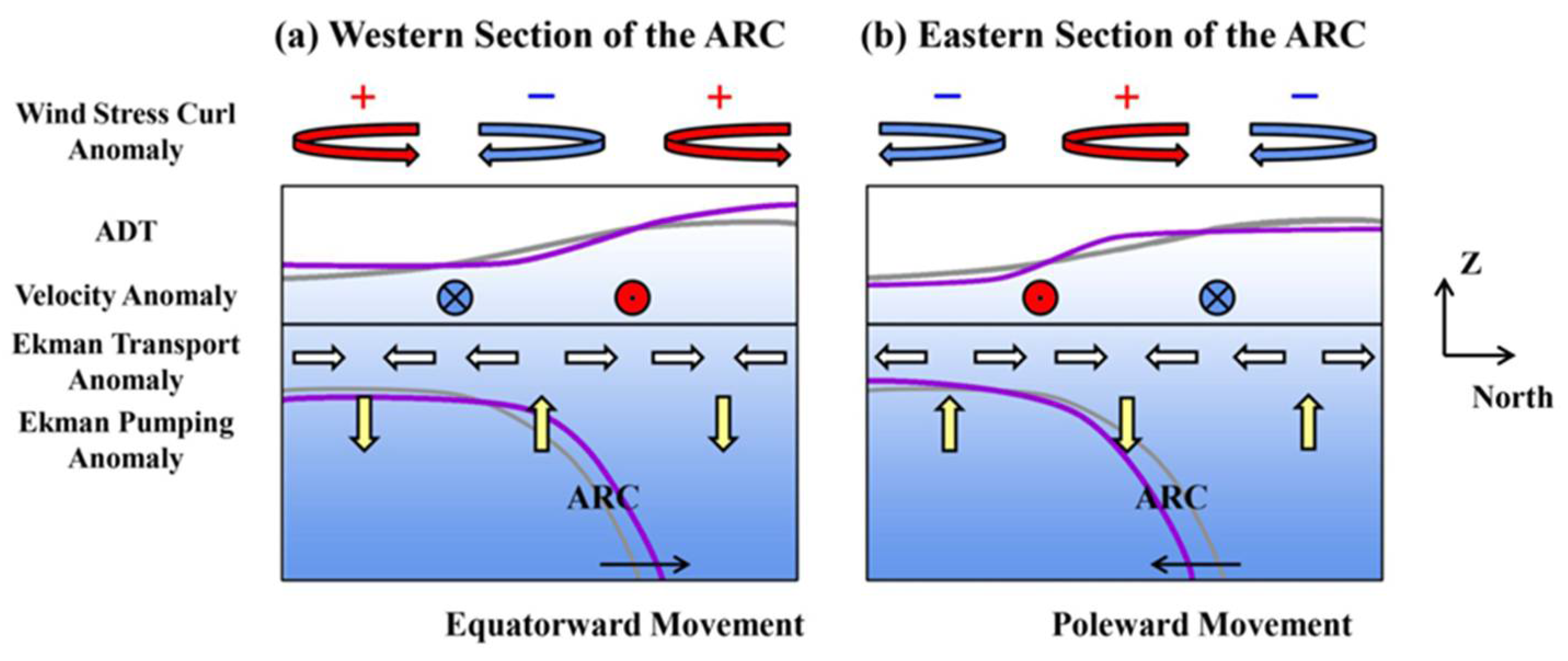
We further explore the underlying mechanism for this slanting trend. It can be briefly depicted in Figure 16: associated with the slanting of the ARC axis, the wind stress curl anomaly in the ARC’s western section has a positive–negative–positive distribution from north to south, generating a positive–negative–positive ADT anomaly distribution through wind-driven Ekman pumping/suction. According to the geostrophic relationship, the change of the ADT meridional gradient will cause the ARC’s velocity anomaly to be positive on the ARC’s north side and negative on the south side, therefore, the ARC’s western section will move northward. Conversely, the negative–positive–negative distribution of wind stress curl anomaly from north to south will result in the southward movement of the ARC’s eastern section. In short, this northwest–southeast slanting tendency of the ARC axis may be attributed to the dynamical adjustment process of the upper ocean’s circulation in response to local wind forcing, with the only exception being the headstream region, where interactions between the mean flow, topography and mesoscale eddies dominate.
The effects of the sloping ARC path on the eddy activity are also explored in this study. The results show that the ARC path movement trend could, at least partly, explain the spatial distribution of the EKE trends in the midstream and downstream of the ARC region. The downstream ARC east of 48°E is more likely to interact with ACC fronts, inducing the EKE response. In contrast, the ARC headstream west of 35°E is more subject to topography; thus, the EKE change manifests mostly in the deformation of the large meanders and is closely related to eddy shedding, propagation and merging processes.
Author Contributions
Conceptualization, Y.L. and X.-Y.Y.; methodology, Y.L.; software, Y.L.; validation, Y.L., L.L., D.W. and X.-Y.Y.; formal analysis, Y.L.; writing—original draft preparation, Y.L.; writing—review and editing, Y.L., L.L., D.W. and X.-Y.Y.; visualization, Y.L. and X.-Y.Y.; supervision, X.-Y.Y.; project administration, X.-Y.Y.; funding acquisition, L.L., D.W. and X.-Y.Y. All authors have read and agreed to the published version of the manuscript.
Funding
This research was funded by the National Key R&D Program of China (2019YFA0606702) and the National Natural Science Foundation China (grant number 42006177, 42176222, 91858202 and 41776003).
Data Availability Statement
The data used in this study are available through various publicly accessible databases. The delayed-time gridded absolute dynamic height dataset can be found at https://resources.marine.copernicus.eu/product-detail/SEALEVEL_GLO_PHY_CLMATE_L4_MY008_057/INFORMATION (accessed on 1 August 2021). The ERA5 surface wind data can be accessed from the Climate Data Store at https://cds.climate.copernicus.eu/#&hx0021;/search?text=ERA5&type=dataset (accessed on 6 January 2021).
Acknowledgments
We thank ECWMF and Copernicus website for providing the data used in this study. We appreciate three anonymous reviewers for their great suggestions and advice to help improve the quality of the paper.
Conflicts of Interest
The authors declare no conflict of interest.
References
- Rouault, M.; Penven, P.; Pohl, B. Warming in the Agulhas Current system since the 1980’s. Geophys. Res. Lett. 2009, 36, L12602. [Google Scholar] [CrossRef]
- Renault, L.; McWilliams, J.C.; Penven, P. Modulation of the Agulhas Current Retroflection and leakage by oceanic current interaction with the atmosphere in coupled simulations. J. Phys. Oceanogr. 2017, 47, 2077–2100. [Google Scholar] [CrossRef]
- Wang, J.; Mazloff, M.R.; Gille, S.T. Pathways of the Agulhas waters poleward of 29°S. J. Geophys. Res.-Ocean. 2014, 119, 4234–4250. [Google Scholar] [CrossRef]
- Rusciano, E.; Speich, S.; Ollitrault, M. Interocean exchanges and the spreading of Antarctic Intermediate Water south of Africa. J. Geophys. Res. Ocean. 2012, 117, C10010. [Google Scholar] [CrossRef]
- Lutjeharms, J.R.E. The Exchange of Water Between the South Indian and South Atlantic Oceans. In The South Atlantic: Present and Past Circulation; Springer: Berlin/Heidelberg, Germany, 1996; pp. 125–162. [Google Scholar]
- Wei, L.; Wang, C. Characteristics of ocean mesoscale eddies in the Agulhas and Tasman Leakage regions from two eddy datasets. Deep. Sea Res. Part II Top. Stud. Oceanogr. 2023, 208, 105264. [Google Scholar] [CrossRef]
- Lutjeharms, J.R.E. The Agulhas Current; Springer: Berlin/Heidelberg, Germany, 2006. [Google Scholar]
- Lutjeharms, J.R.E.; Van Ballegooyen, R.C. Topographic Control in the Agulhas Current System. Deep. Sea Res. Part A Oceanogr. Res. Pap. 1984, 31, 1321–1337. [Google Scholar] [CrossRef]
- Biastoch, A.; Boning, C.W.; Schwarzkopf, F.U.; Lutjeharms, J.R. Increase in Agulhas leakage due to poleward shift of Southern Hemisphere westerlies. Nature 2009, 462, 495–498. [Google Scholar] [CrossRef] [PubMed]
- Van Sebille, E.; Barron, C.N.; Biastoch, A.; van Leeuwen, P.J.; Vossepoel, F.C.; de Ruijter, W.P.M. Relating Agulhas leakage to the Agulhas Current retroflection location. Ocean. Sci. 2009, 5, 511–521. [Google Scholar] [CrossRef]
- Durgadoo, J.V.; Loveday, B.R.; Reason, C.J.C.; Penven, P.; Biastoch, A. Agulhas Leakage Predominantly Responds to the Southern Hemisphere Westerlies. J. Phys. Oceanogr. 2013, 43, 2113–2131. [Google Scholar] [CrossRef]
- Loveday, B.R.; Durgadoo, J.V.; Reason, C.J.C.; Biastoch, A.; Penven, P. Decoupling of the Agulhas Leakage from the Agulhas Current. J. Phys. Oceanogr. 2014, 44, 1776–1797. [Google Scholar] [CrossRef]
- Beal, L.M.; de Ruijter, W.P.; Biastoch, A.; Zahn, R.; Group, S.W.I.W. On the role of the Agulhas system in ocean circulation and climate. Nature 2011, 472, 429–436. [Google Scholar] [CrossRef] [PubMed]
- Drijfhout, S.S.; Blaker, A.T.; Josey, S.A.; Nurser, A.J.G.; Sinha, B.; Balmaseda, M.A. Surface warming hiatus caused by increased heat uptake across multiple ocean basins. Geophys. Res. Lett. 2014, 41, 7868–7874. [Google Scholar] [CrossRef]
- de Ruijter, W.P.M.; Aken, H.M.V.; Beier, E.J.; Lutjeharms, J.R.E.; Matano, R.P.; Schouten, M.W. Eddies and dipoles around South Madagascar: Formation, pathways and large-scale impact. Deep. Sea Res. Part I Oceanogr. Res. Pap. 2004, 51, 383–400. [Google Scholar] [CrossRef]
- Dencausse, G.; Arhan, M.; Speich, S. Spatio-temporal characteristics of the Agulhas Current retroflection. Deep. Sea Res. Part I Oceanogr. Res. Pap. 2010, 57, 1392–1405. [Google Scholar] [CrossRef]
- Van Sebille, E.; Biastoch, A.; van Leeuwen, P.J.; de Ruijter, W.P.M. A weaker Agulhas Current leads to more Agulhas leakage. Geophys. Res. Lett. 2009, 36, L03601. [Google Scholar] [CrossRef]
- Siedler, G.; Rouault, M.; Biastoch, A.; Backeberg, B.; Reason, C.J.C.; Lutjeharms, J.R.E. Modes of the southern extension of the East Madagascar Current. J. Geophys. Res. Ocean. 2009, 114, C01005. [Google Scholar] [CrossRef]
- Zhu, Y.; Li, Y.; Zhang, Z.; Qiu, B.; Wang, F. The observed Agulhas Retroflection behaviors during 1993–2018. J. Geophys. Res. Ocean. 2021, 126, e2021JC017995. [Google Scholar] [CrossRef]
- Backeberg, B.C.; Penven, P.; Rouault, M. Impact of intensified Indian Ocean winds on mesoscale variability in the Agulhas system. Nat. Clim. Chang. 2012, 2, 608–612. [Google Scholar] [CrossRef]
- Lutjeharms, J.R.E.; Van Ballegooyen, R.C. The Retroflection of the Agulhas Current. J. Phys. Oceanogr. 1988, 18, 1570–1583. [Google Scholar] [CrossRef]
- Le Bars, D.; Ruijter, W.P.M.; Dijkstra, H. A New Regime of the Agulhas Current Retroflection: Turbulent Choking of Indian–Atlantic leakage. J. Phys. Oceanogr. 2012, 42, 1158–1172. [Google Scholar] [CrossRef]
- Sallee, J.B.; Speer, K.; Morrow, R. Response of the Antarctic Circumpolar Current to atmospheric variability. J. Clim. 2008, 21, 3020–3039. [Google Scholar] [CrossRef]
- Domingues, R.; Goni, G.; Swart, S.; Dong, S.F. Wind forced variability of the Antarctic Circumpolar Current south of Africa between 1993 and 2010. J. Geophys. Res. Ocean. 2014, 119, 1123–1145. [Google Scholar] [CrossRef]
- Yang, H.; Lohmann, G.; Wei, W.; Dima, M.; Ionita, M.; Liu, J. Intensification and poleward shift of subtropical western boundary currents in a warming climate. J. Geophys. Res. Ocean. 2016, 121, 4928–4945. [Google Scholar] [CrossRef]
- Yang, H.; Lohmann, G.; Krebs-Kanzow, U.; Ionita, M.; Shi, X.X.; Sidorenko, D.; Gong, X.; Chen, X.E.; Gowan, E.J. Poleward Shift of the Major Ocean Gyres Detected in a Warming Climate. Geophys. Res. Lett. 2020, 47, e2019GL085868. [Google Scholar] [CrossRef]
- Qiu, B.; Chen, S.M.; Schneider, N.; Oka, E.; Sugimoto, S. On the Reset of the Wind-Forced Decadal Kuroshio Extension Variability in Late 2017. J. Clim. 2020, 33, 10813–10828. [Google Scholar] [CrossRef]
- Fadida, Y.; Malan, N.; Cronin, M.F.; Hermes, J. Trends in the Agulhas Return Current. Deep. Sea Res. Part I Oceanogr. Res. Pap. 2021, 175, 103573. [Google Scholar] [CrossRef]
- Rio, M.H.; Santoleri, R. Improved global surface currents from the merging of altimetry and Sea Surface Temperature data. Remote Sens. Environ. 2018, 216, 770–785. [Google Scholar] [CrossRef]
- Mulet, S.; Rio, M.H.; Etienne, H.; Artana, C.; Cancet, M.; Dibarboure, G.; Feng, H.; Husson, R.; Picot, N.; Provost, C.; et al. The new CNES-CLS18 global mean dynamic topography. Ocean Sci. 2021, 17, 789–808. [Google Scholar] [CrossRef]
- Hersbach, H.; Bell, B.; Berrisford, P.; Hirahara, S.; Horányi, A.; Muñoz-Sabater, J.; Nicolas, J.; Peubey, C.; Radu, R.; Schepers, D.; et al. The ERA5 global reanalysis. Q. J. R. Meteorol. Soc. 2020, 146, 1999–2049. [Google Scholar] [CrossRef]
- Cummings, J.A. Operational multivariate ocean data assimilation. Q. J. R. Meteorol. Soc. 2005, 131, 3583–3604. [Google Scholar] [CrossRef]
- Cummings, J.A.; Smedstad, O.M. Variational Data Assimilation for the Global Ocean. In Data Assimilation for Atmospheric, Oceanic and Hydrologic Applications; Springer: Berlin/Heidelberg, Germany, 2013; Volume II, Chapter 13; pp. 303–343. [Google Scholar]
- Qiu, B.; Chen, S.M. Variability of the Kuroshio Extension jet, recirculation gyre, and mesoscale eddies on decadal time scales. J. Phys. Oceanogr. 2005, 35, 2090–2103. [Google Scholar] [CrossRef]
- Clifford, M.A. A Descriptive Study of the Zonation of the Antarctic Circumpolar Current and Its Relation to Wind Stress and Ice Cover. Ph.D. Thesis, Texas A&M University, College Station, TX, USA, 1983. [Google Scholar]
- Zhu, Y.N.; Qiu, B.; Lin, X.P.; Wang, F. Interannual Eddy Kinetic Energy Modulations in the Agulhas Return Current. J. Geophys. Res.-Oceans 2018, 123, 6449–6462. [Google Scholar] [CrossRef]
- Boebel, O.; Rossby, T.; Lutjeharms, J.; Zenk, W.; Barron, C. Path and variability of the Agulhas Return Current. Deep. Sea Res. Part II Top. Stud. Oceanogr. 2003, 50, 35–56. [Google Scholar] [CrossRef]
Figure 1.
Definition of the ARC jet axis. (a) The geographic distribution of climatological geostrophic velocity during 1993–2020 (shading in m/s). The thin black lines represent the climatology ADT contours (contour interval: 0.1 m), and the thick black line represents the 0.7 m contour. (b) The geographic distribution of geostrophic velocity in January 1993 (shading in m/s). The two blue lines indicate the southern and northern boundaries of the search area, and the red line indicates the search result.

Figure 2.
The ARC path movement trend. (a) The geographic distribution of geostrophic velocity trend during 1993–2020 (shading in (m/s)/year). The thin black lines represent the climatology ADT contours (contour interval: 0.1 m), and the thick black line indicates the mean jet axis defined by the ADT maximum gradient method. Stippling regions indicate the trends that are statistically significant (p-value < 0.05). (b) Trends of the meridional migration of the ARC during 1993–2020 (solid black line in °/year). The dashed grey line is the zero line, and the red circles indicate that the trends are significant (p < 0.05).

Figure 3.
Time series (solid black line) and linear trend (dashed red line, significant at the 0.05 level) of the ARC movement index (AMI). Red asterisks indicate high AMI, and green asterisks indicate low AMI.
Figure 3.
Time series (solid black line) and linear trend (dashed red line, significant at the 0.05 level) of the ARC movement index (AMI). Red asterisks indicate high AMI, and green asterisks indicate low AMI.
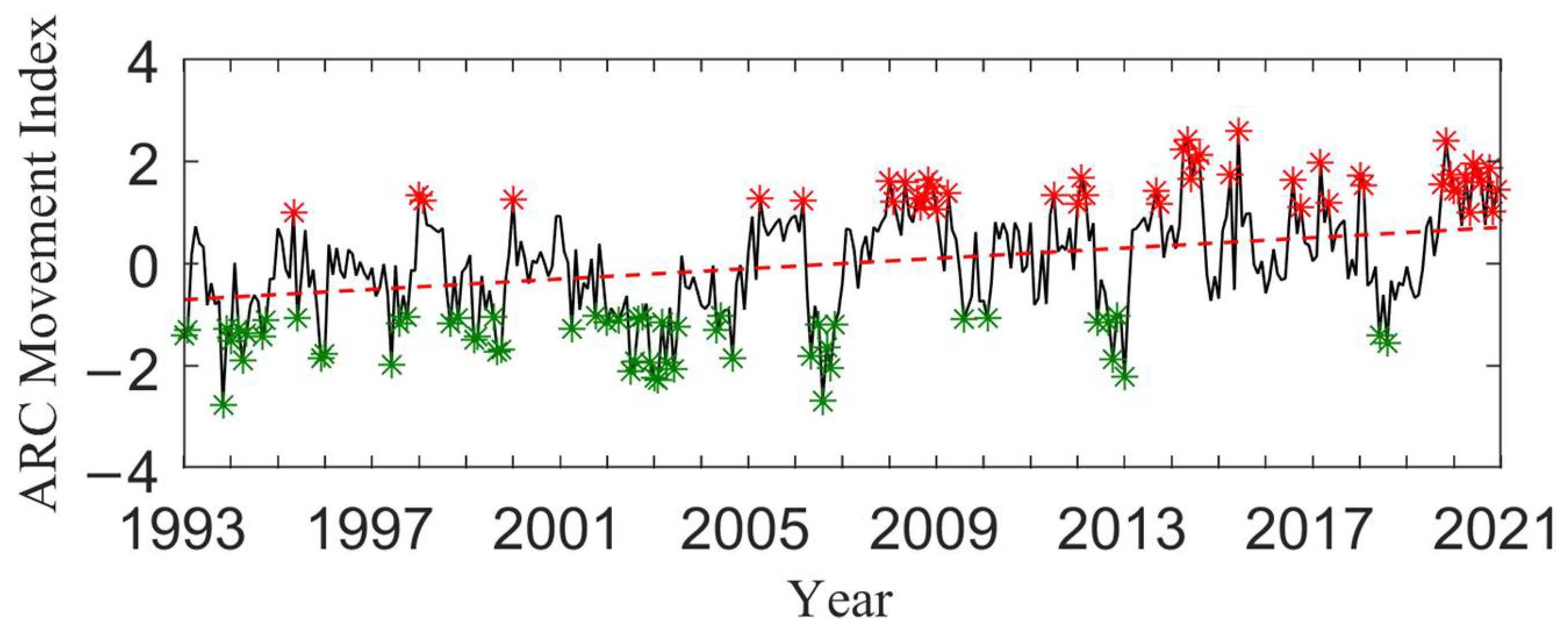
Figure 4.
The composite of geostrophic velocity (shading in m/s and vector) in different AMI phases. (a) AMI positive phase. (b) AMI negative phase. The red and green lines denote the mean ARC axis for the AMI positive phase and negative phase, respectively. The gray, thin lines denote the climatology of ADT contours.
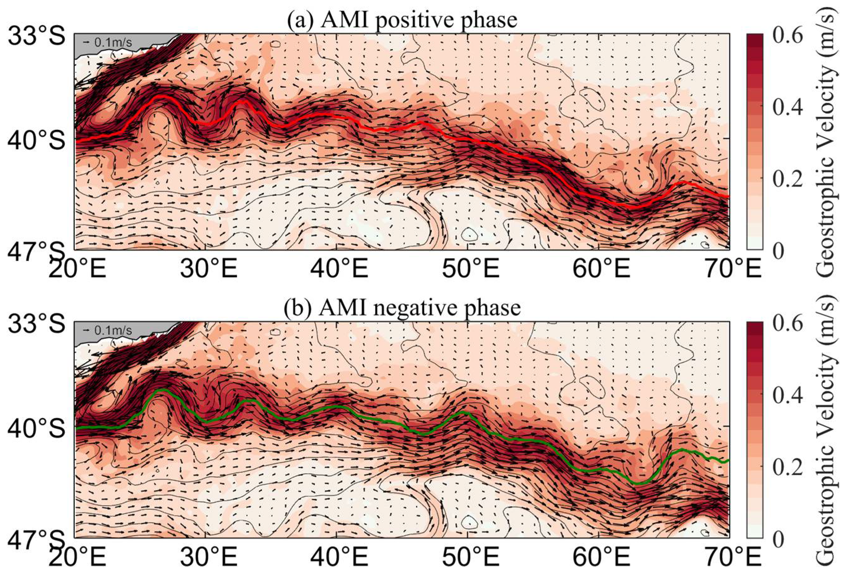
Figure 5.
Seasonal cycle of the ARC positions in °N. The solid green, red, yellow, and blue lines represent the average ARC positions during austral spring (September–November), summer (December–February), autumn (March–May), and winter (June–August), respectively. The yellow and purple dotted lines represent the longitudes of the ARC troughs and crests, respectively.
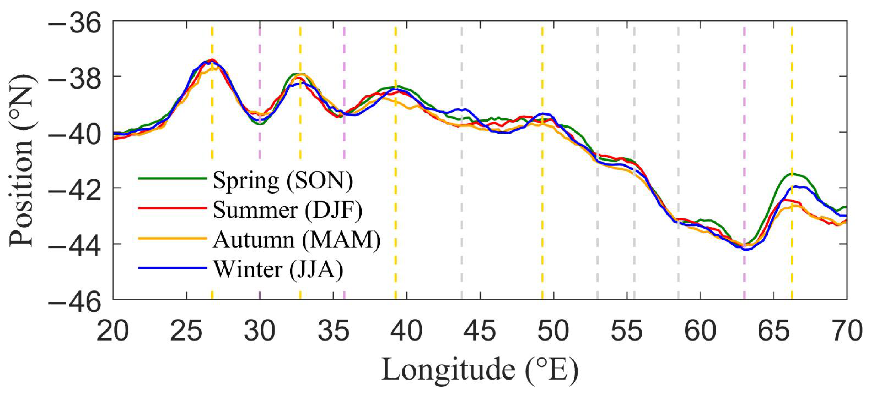
Figure 6.
The composite of ADT (shading in m) and geostrophic velocity (vector, p-value < 0.05) difference fields between the extreme positive and negative phase of the ARC movement index. The gray, thin lines are the climatology of ADT contours. The blue and red, thick lines designate the ADT difference equal to −0.1 m and 0.1 m, respectively. Stippling regions indicate the composites that are statistically significant (p-value < 0.05).
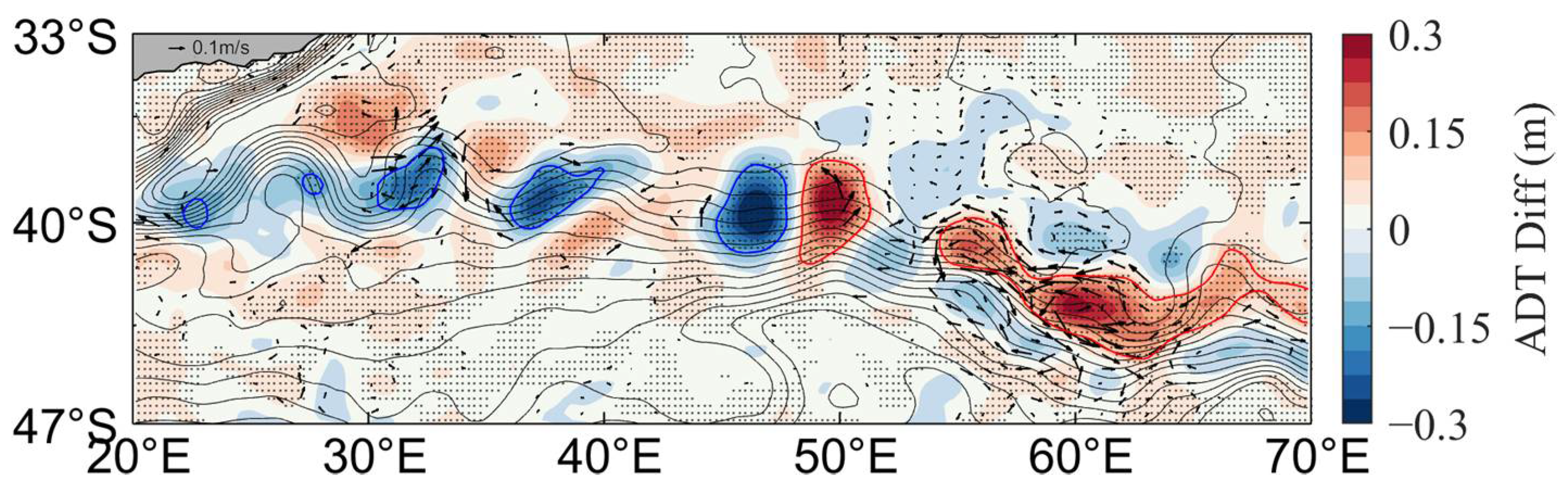
Figure 7.
Composites of wind stress curl anomalies integral along the ADT contours, based on the AMI (unit in N/m3). (a) The western section of the ARC. (b) The eastern section of the ARC.
Figure 7.
Composites of wind stress curl anomalies integral along the ADT contours, based on the AMI (unit in N/m3). (a) The western section of the ARC. (b) The eastern section of the ARC.
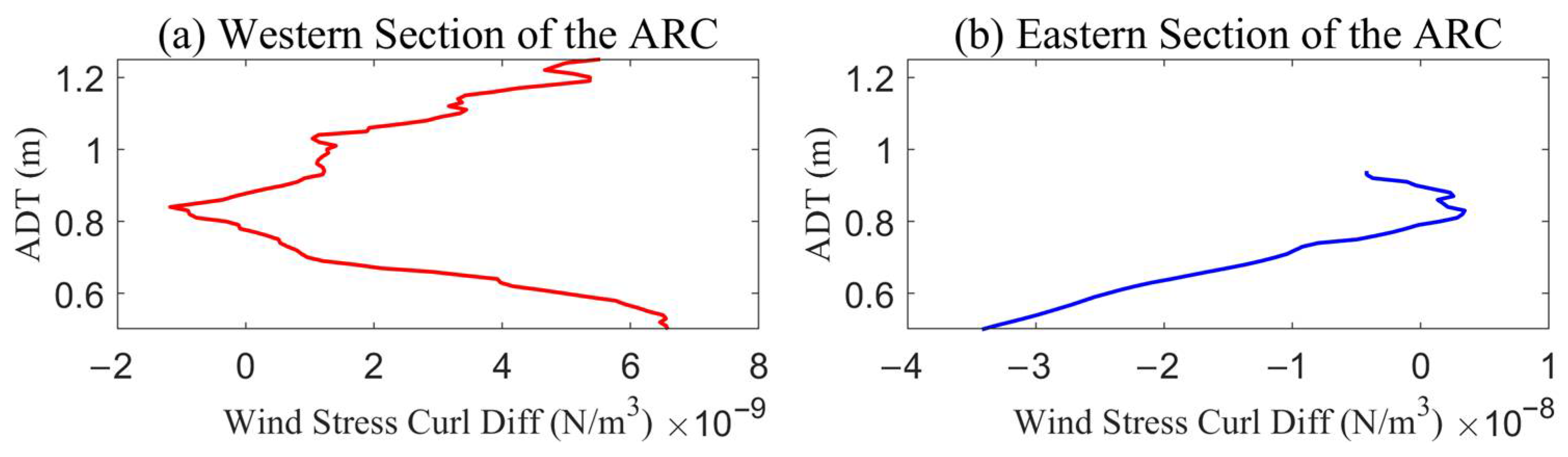
Figure 8.
The geographic distribution of the EKE trend during 1993–2020 (shading in (m2/s2)/year). The black lines represent the climatology ADT contours, the thick black line is the mean jet axis, and stippling regions indicate the trends that are statistically significant (p-value < 0.05).
Figure 8.
The geographic distribution of the EKE trend during 1993–2020 (shading in (m2/s2)/year). The black lines represent the climatology ADT contours, the thick black line is the mean jet axis, and stippling regions indicate the trends that are statistically significant (p-value < 0.05).
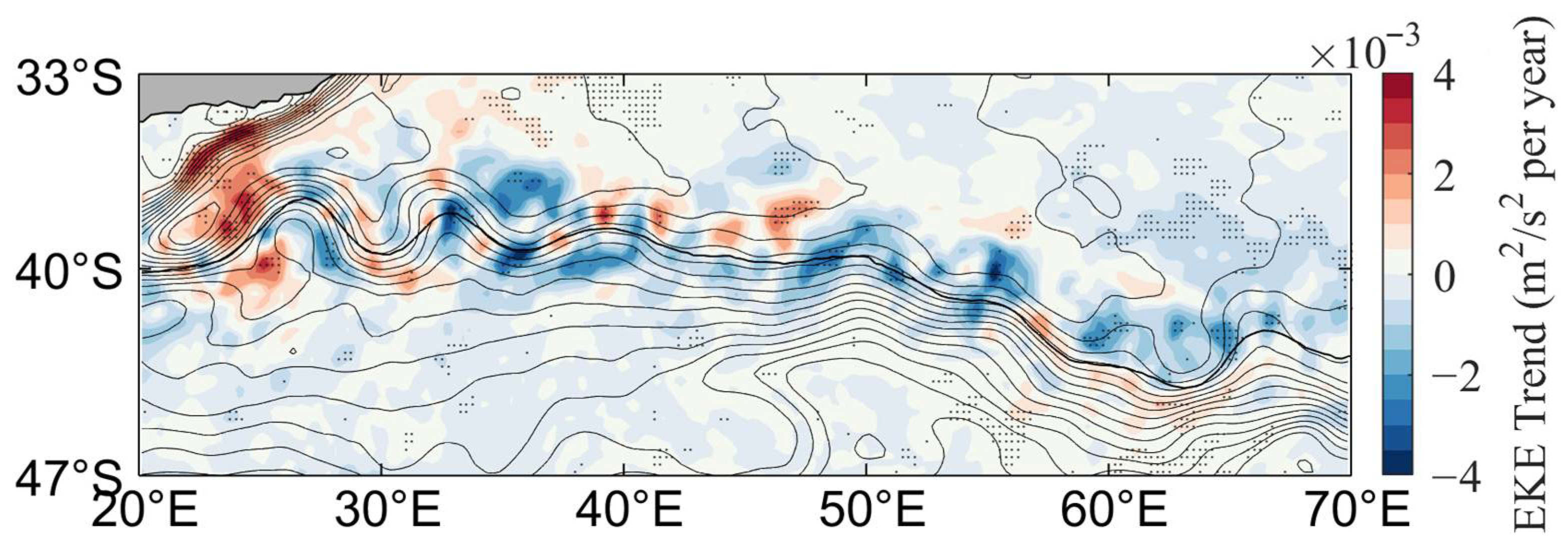
Figure 9.
Regression of EKE anomalies onto the AMI (shading). The black lines denote the climatology ADT contours, the thick black line denotes the mean jet axis, and the stippling regions indicate the regression coefficients that are statistically significant (p-value < 0.05).
Figure 9.
Regression of EKE anomalies onto the AMI (shading). The black lines denote the climatology ADT contours, the thick black line denotes the mean jet axis, and the stippling regions indicate the regression coefficients that are statistically significant (p-value < 0.05).
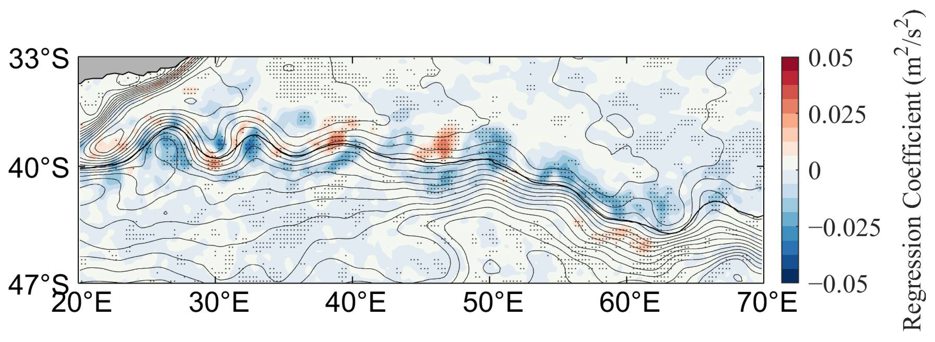
Figure 10.
The climatological locations of the ARC (red line), the STF (gray line), and the SAF (blue line).
Figure 10.
The climatological locations of the ARC (red line), the STF (gray line), and the SAF (blue line).
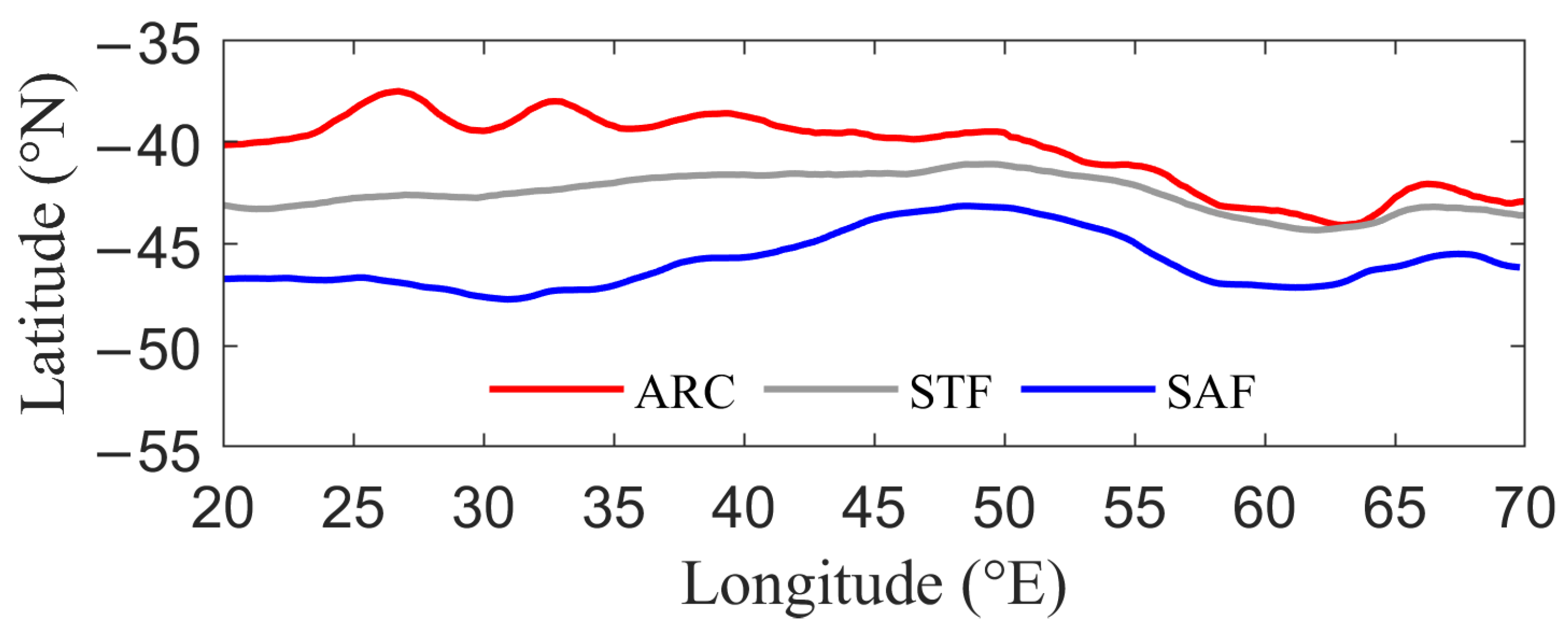
Figure 11.
ARC topographical meandering. (a–d) Average ADT fields (shading in m) and jet axes (black lines) during 1993–1999, 2000–2006, 2007–2013, and 2014–2020, respectively. The grey lines are isobaths. T1 and T2 in (d) indicate the positions of the first and second troughs; C0 indicates the ARC meander above the Agulhas Plateau, and C1 indicates the position of the first crest. The blue boxes labeled with numbers from 1 to 4 are the four regions used to construct the ARC deformation index (ADI).
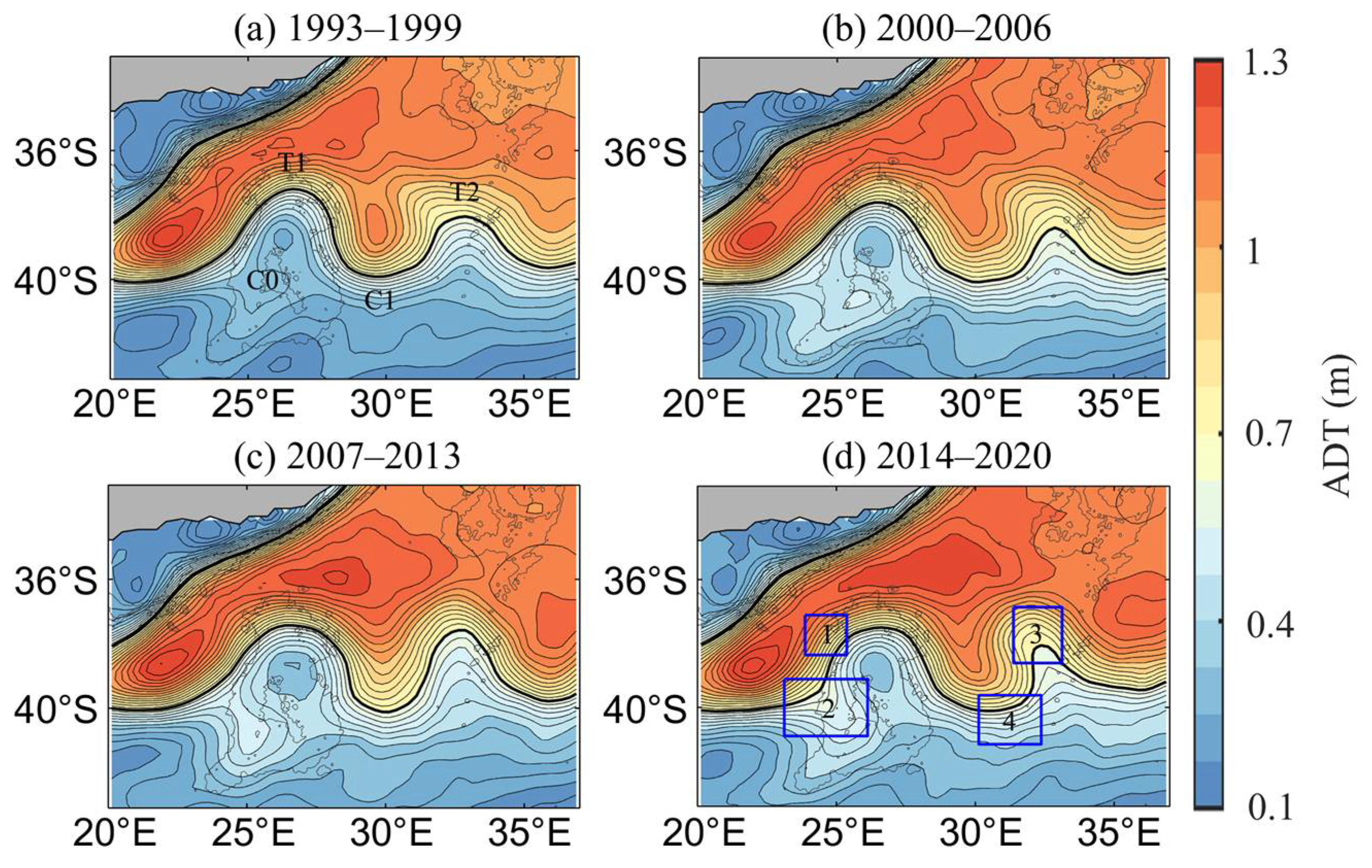
Figure 12.
Time series (solid black line) and linear trend (dashed red line, significant at the 0.05 level) of the ARC deformation index (ADI). Red asterisks indicate high ADI, and green asterisks indicate low ADI.
Figure 12.
Time series (solid black line) and linear trend (dashed red line, significant at the 0.05 level) of the ARC deformation index (ADI). Red asterisks indicate high ADI, and green asterisks indicate low ADI.
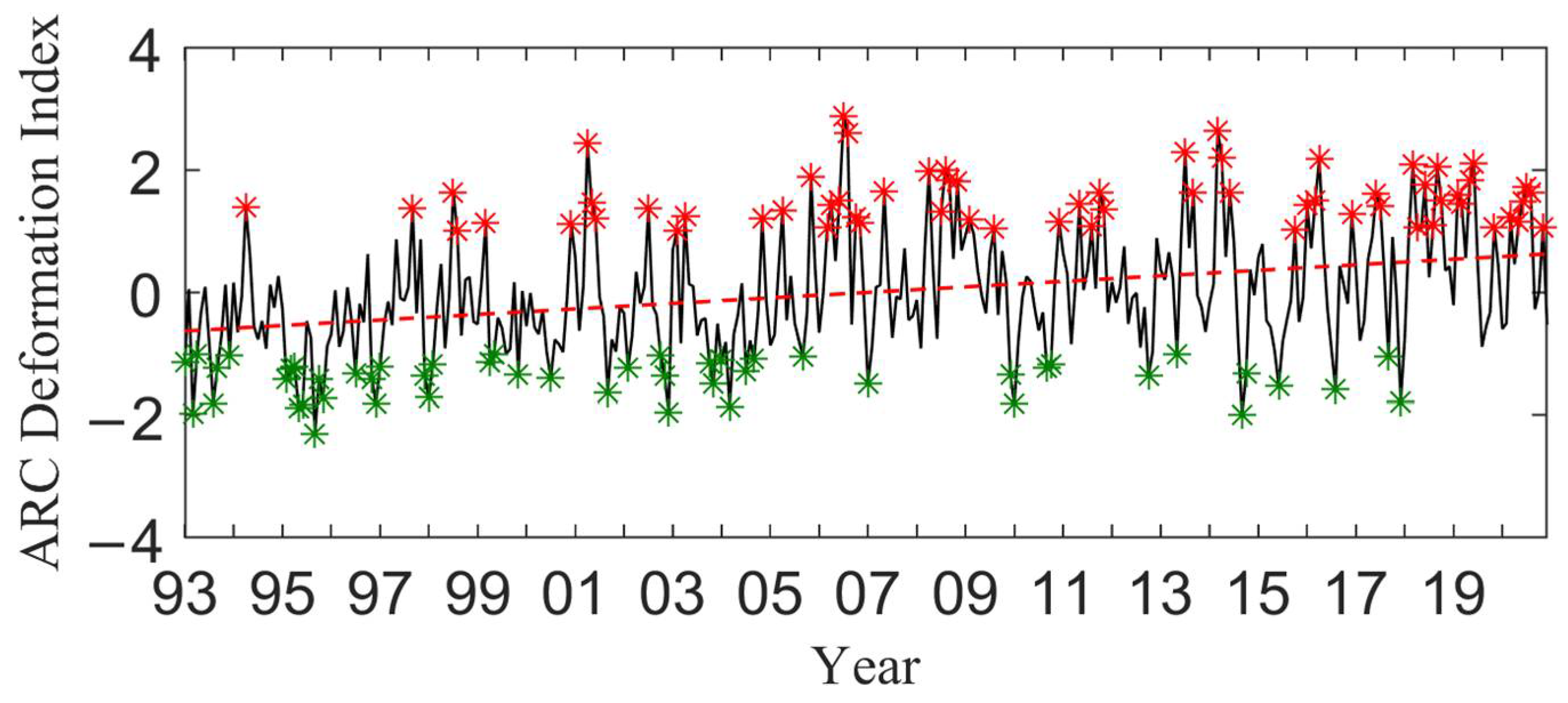
Figure 13.
The composite fields of ADT (shading in m) and geostrophic velocity (vector) in the extreme months of the ARC deformation index. (a) Positive phase. (b) Negative phase.
Figure 13.
The composite fields of ADT (shading in m) and geostrophic velocity (vector) in the extreme months of the ARC deformation index. (a) Positive phase. (b) Negative phase.
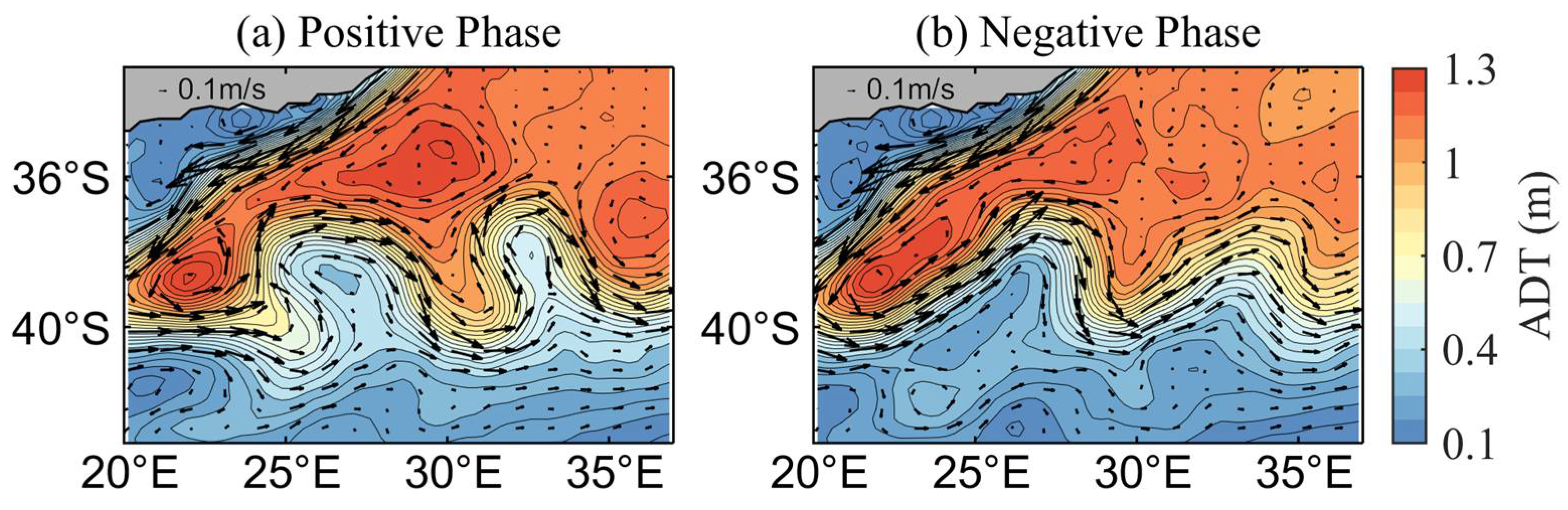
Figure 14.
The seasonal cycle of the ARC deformation index.
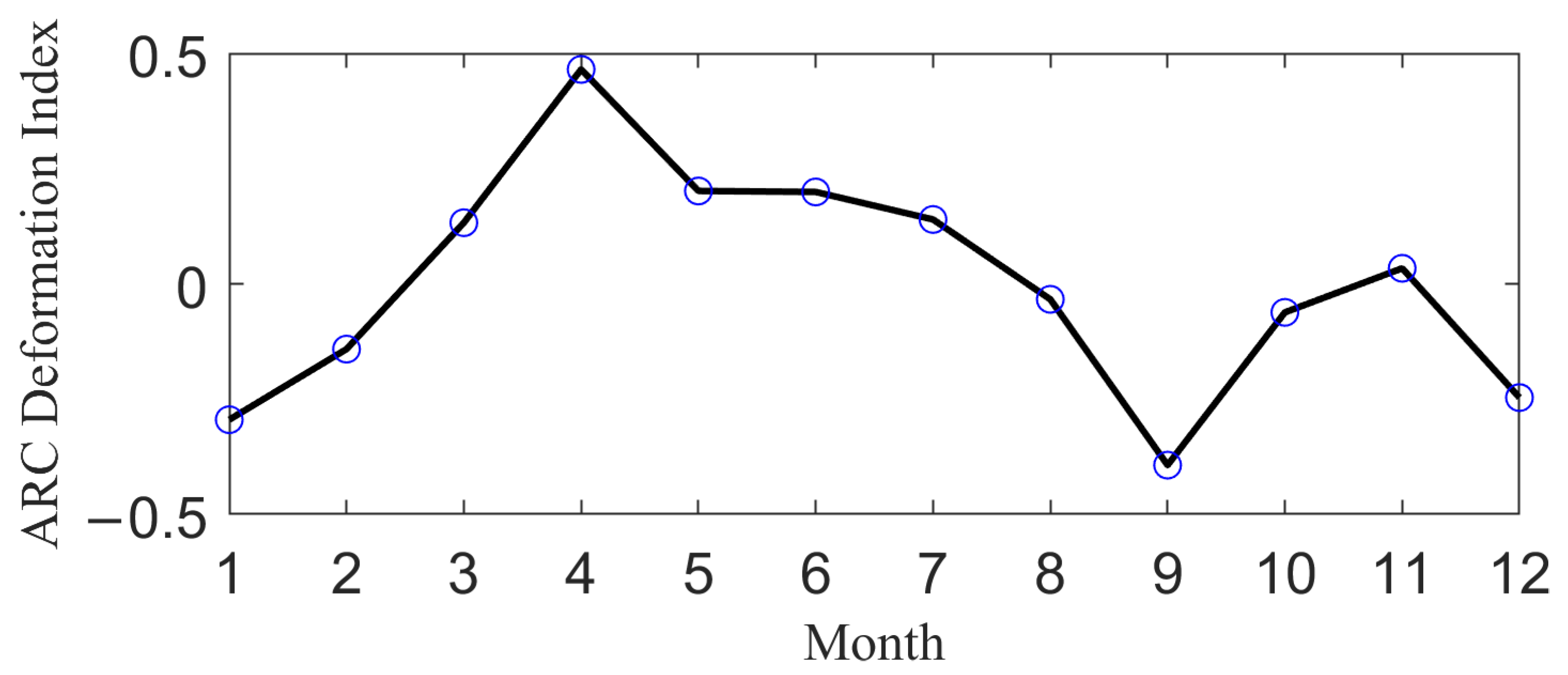
Figure 15.
Regression of EKE anomalies onto the ADI (shading). The black lines are the climatology ADT contours, the thick black line is the mean jet axis, and stippling regions indicate the regression coefficients that are statistically significant (p-value < 0.05).
Figure 15.
Regression of EKE anomalies onto the ADI (shading). The black lines are the climatology ADT contours, the thick black line is the mean jet axis, and stippling regions indicate the regression coefficients that are statistically significant (p-value < 0.05).
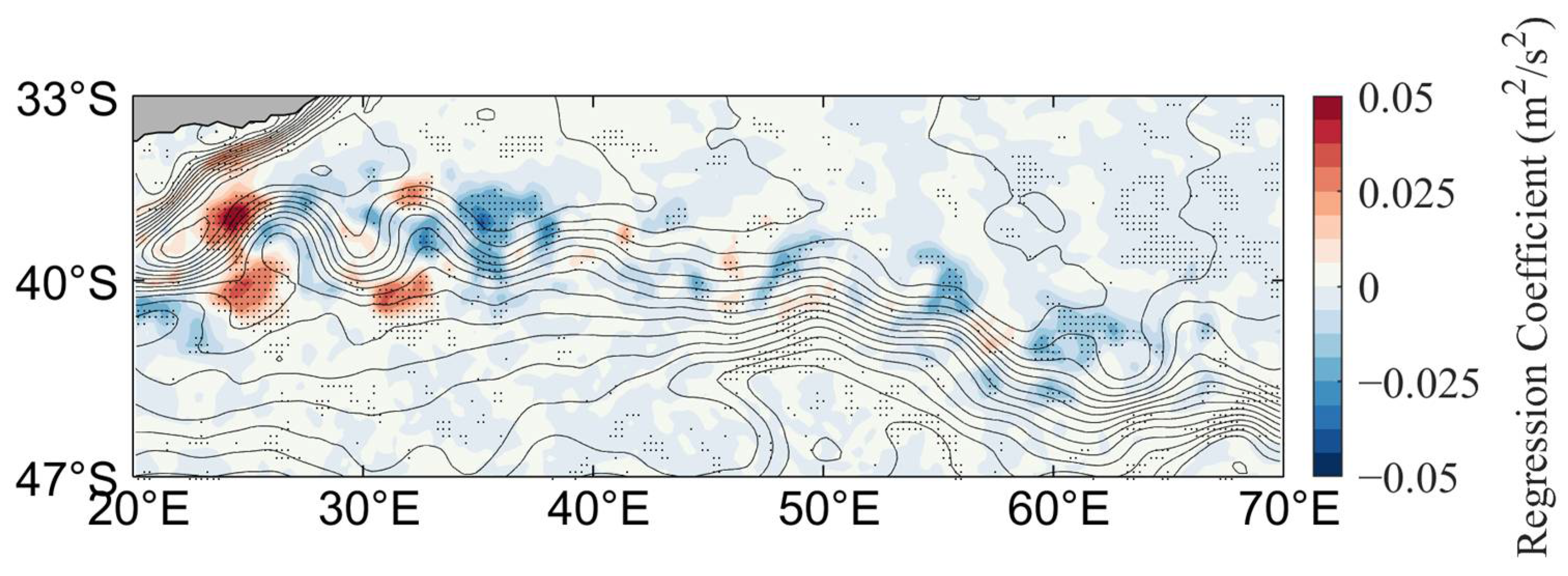
Figure 16.
A schematic of the mechanism of the ARC path movement in its positive phase. (a) The western section of the ARC. (b) The eastern section of the ARC. The red and blue arrows represent the positive and negative wind stress curl anomalies; the red and blue symbols on the vertical paper represent the positive and negative geostrophic velocity anomalies; the white and yellow arrows represent the Ekman transport anomalies and Ekman pumping anomalies; the gray lines represent the climatology ADT (above) and the ARC isopycnal (below), the purple lines represent the ADT (above) and the ARC isopycnal (below) in response to the wind stress curl anomalies; the black arrows show the directions of the ARC movement.
Disclaimer/Publisher’s Note: The statements, opinions and data contained in all publications are solely those of the individual author(s) and contributor(s) and not of MDPI and/or the editor(s). MDPI and/or the editor(s) disclaim responsibility for any injury to people or property resulting from any ideas, methods, instructions or products referred to in the content. |
© 2023 by the authors. Licensee MDPI, Basel, Switzerland. This article is an open access article distributed under the terms and conditions of the Creative Commons Attribution (CC BY) license (https://creativecommons.org/licenses/by/4.0/).
Share and Cite
MDPI and ACS Style
Lin, Y.; Lin, L.; Wang, D.; Yang, X.-Y. Inclination Trend of the Agulhas Return Current Path in Three Decades. Remote Sens. 2023, 15, 5652. https://doi.org/10.3390/rs15245652
AMA Style
Lin Y, Lin L, Wang D, Yang X-Y. Inclination Trend of the Agulhas Return Current Path in Three Decades. Remote Sensing. 2023; 15(24):5652. https://doi.org/10.3390/rs15245652
Chicago/Turabian StyleLin, Yan, Liru Lin, Dongxiao Wang, and Xiao-Yi Yang. 2023. "Inclination Trend of the Agulhas Return Current Path in Three Decades" Remote Sensing 15, no. 24: 5652. https://doi.org/10.3390/rs15245652
Note that from the first issue of 2016, this journal uses article numbers instead of page numbers. See further details here.