Article

A Green Fingerprint of Antarctica: Drones, Hyperspectral Imaging, and Machine Learning for Moss and Lichen Classification

1
Securing Antarctica’s Environmental Future, Queensland University of Technology, 2 George St, Brisbane City, QLD 4000, Australia
2
QUT Centre For Robotics, Queensland University of Technology, 2 George St, Brisbane City, QLD 4000, Australia
3
Securing Antarctica’s Environmental Future, University of Wollongong, Northfields Ave, Wollongong, NSW 2522, Australia
4
School of Earth, Atmospheric and Life Sciences, University of Wollongong, Northfields Ave, Wollongong, NSW 2522, Australia
5
NVIDIA, Santa Clara, CA 95051, USA
*
Author to whom correspondence should be addressed.
Remote Sens. 2023, 15(24), 5658; https://doi.org/10.3390/rs15245658
Submission received: 31 October 2023 / Revised: 27 November 2023 / Accepted: 4 December 2023 / Published: 7 December 2023
(This article belongs to the Special Issue Antarctic Remote Sensing Applications)

Abstract

:
Mapping Antarctic Specially Protected Areas (ASPAs) remains a critical yet challenging task, especially in extreme environments like Antarctica. Traditional methods are often cumbersome, expensive, and risky, with limited satellite data further hindering accuracy. This study addresses these challenges by developing a workflow that enables precise mapping and monitoring of vegetation in ASPAs. The processing pipeline of this workflow integrates small unmanned aerial vehicles (UAVs)—or drones—to collect hyperspectral and multispectral imagery (HSI and MSI), global navigation satellite system (GNSS) enhanced with real-time kinematics (RTK) to collect ground control points (GCPs), and supervised machine learning classifiers. This workflow was validated in the field by acquiring ground and aerial data at ASPA 135, Windmill Islands, East Antarctica. The data preparation phase involves a data fusion technique to integrate HSI and MSI data, achieving the collection of georeferenced HSI scans with a resolution of up to 0.3 cm/pixel. From these high-resolution HSI scans, a series of novel spectral indices were proposed to enhance the classification accuracy of the model. Model training was achieved using extreme gradient boosting (XGBoost), with four different combinations tested to identify the best fit for the data. The research results indicate the successful detection and mapping of moss and lichens, with an average accuracy of 95%. Optimised XGBoost models, particularly Model 3 and Model 4, demonstrate the applicability of the custom spectral indices to achieve high accuracy with reduced computing power requirements. The integration of these technologies results in significantly more accurate mapping compared to conventional methods. This workflow serves as a foundational step towards more extensive remote sensing applications in Antarctic and ASPA vegetation mapping, as well as in monitoring the impact of climate change on the Antarctic ecosystem.

1. Introduction

Antarctica is home to a unique and diverse ecosystem that is sensitive to climate change, extreme events, and human activities [1,2,3,4,5,6,7,8,9]. Vegetation, such as mosses and lichens, plays a vital role in maintaining the ecological balance, insulating ice-free soils, biogeochemical cycling, and providing habitat for much of Antarctica’s terrestrial biodiversity [3,10,11,12,13,14,15]. However, mapping and monitoring vegetation in Antarctica presents challenges due to its remoteness, harsh environment, limited accessibility, and a changing climate [2,6,16,17]. Traditional methods of field surveys prove to be time-consuming, costly, and risky, potentially causing disturbance to the fragile vegetation [17]. While satellite imagery is widely available, it has limitations in spatial and spectral resolution, cloud cover, and temporal frequency [12,17,18,19,20].
Recent advances in remote sensing technologies offer opportunities to address these challenges, enabling more accurate and efficient mapping and monitoring at scales relevant to vegetation in Antarctica. Specifically, unmanned aerial vehicles (UAVs)—or drones—equipped with multispectral and hyperspectral cameras can provide high-resolution imagery with rich spectral information over extensive areas in a flexible and safe manner [19,20,21,22,23]. Additionally, machine learning (ML) techniques have the potential to harness the capabilities of MSI and HSI data to classify various vegetation types and assess their health condition [24,25].
Nevertheless, several gaps and challenges persist in applying these technologies to Antarctic vegetation mapping. Notably, there is an absence of standardised workflows that integrate UAVs, multispectral (MSI) and hyperspectral (HSI) imagery, and ML models into vegetation classification. A demand exists for innovative spectral indices and features that can highlight the unique characteristics of Antarctic vegetation [17,19,20,24,26]. King et al. [17] discusses the need for remote/passive monitoring techniques to be developed for vegetation monitoring. Moreover, a scarcity of ground truth data and validation methods hinders the evaluation of model performance [12].
Research on UAV imagery resolution for Antarctic vegetation is valuable but limited. For instance, Turner et al. [27] advanced the understanding of spectral and spatial resolutions; yet, their focus may neglect factors like temporal resolution and changing Antarctic conditions. The 2014 studies by Turner et al. [28] and Lucieer et al. [29] demonstrated the potential of micro-UAVs for detailed imaging of moss beds, but faced logistical and technological constraints. These works are limited by the practical challenges of conducting research in remote Antarctic locations and the specific UAV technologies used, which might not be universally applicable.
This study addresses these gaps by introducing and validating a workflow that enables remote sensing of vegetation in extreme environments using UAVs, MSI and HSI data, and supervised ML classification. The workflow encompasses five pivotal phases: (1) data collection; (2) data preparation; (3) feature extraction; (4) model training; and (5) prediction. This approach underwent testing in a case study focusing on lichen detection and moss health classification in an Antarctic Specially Protected Area (ASPA) 135 [30], situated on the Bailey Peninsula in the Windmill Islands region of East Antarctica. Aerial and ground data were gathered using custom-built UAVs and HSI cameras, followed by data processing using fusion techniques to achieve georeferenced HSI scans with superior spatial and spectral resolutions. The subsequent steps involved extracting various spectral indices and statistical features from the labelled images, training four distinct XGBoost models with varying feature combinations, and comparing the generated prediction maps. The processing pipeline contains data fusion techniques to integrate ground HSI scans into georeferenced aerial MSI maps, enhancing data labelling efforts to map moss and lichen using a ground sampling distance (GSD) of up to 0.3 cm/pixel.
The primary contributions of this study include the following:
  • The introduction of a unique workflow that amalgamates UAVs, MSI and HSI data, and ML classifiers for vegetation mapping in Antarctica.
  • The development of a series of innovative spectral indices to amplify the classification precision of Antarctic vegetation.
  • The execution of a field experiment in ASPA 135 to gather aerial and ground data via custom-built UAVs and HSI cameras.
  • The achievement of high accuracy results (95% to 98%) in lichen detection and the classification of moss health using XGBoost models.
The subsequent sections of this paper are structured as follows: Section 2 delves into the details of the proposed workflow; Section 3 outlines the experimental setup and data collection methodologies; Section 4 and Section 5 present the results and discussions related to the models; and Section 6 offers concluding remarks and potential avenues for future research.

2. Remote Sensing Workflow

This study presents a multifaceted workflow that enables the remote sensing of vegetation in extreme environments, leveraging the power of MSI and HSI data captured via UAVs and complemented with terrestrial ground control points (GCPs) for enhanced accuracy and geolocation. The workflow is validated with a case study to detect lichen and classify the health condition of moss. However, the systematic workflow approach presented in this paper can be applied to a diverse range of vegetation types located in polar regions. A holistic illustration of the workflow is displayed in Figure 1.

2.1. Data Collection

Data collection involves a dual-method approach, combining aerial data from UAVs with multispectral and hyperspectral cameras for broad-area surveillance, and ground-level data. Simultaneously, acquiring on-ground data involves various types of sensors and instruments. Before and after UAV flights, white reference samples are collected for accurate reflectance orthomosaics. GCP markers are placed for georeferencing MSI mosaics via global navigation satellite system (GNSS) devices enhanced with real-time kinematics (RTK), and to validate labelled imagery, as detailed in Section 3.5. Ground HSI scans are also georeferenced, providing a data-rich set with high spatial and spectral resolutions, crucial for analysing Antarctic biodiversity variations related to altitude and scale.

2.2. Data Preparation

In this phase, raw data are processed into precise, georeferenced datasets with centimetre-level accuracy. The products are high-resolution MSI orthomosaics used as reference layers. These layers overlay HSI transects for geographic alignment. The phase ends with a list of hyperspectral scans, aerial and ground-based, with pixels aligned to the visual representation of other sensors, creating an integrated dataset.

2.3. Feature Extraction

The feature extraction phase is central to the workflow, yielding data for machine learning models and statistical analysis of classes from HSI data. After spatial and spectral filtering, georeferenced labelled pixels, spectral indices, and statistical features are derived from GCP RTK data, validating the image labelling. These features distinguish regions in the images, enhancing classification precision and robustness.

2.4. Model Training

During model training, this approach optimises one or more supervised ML models and gathers relevant statistics on model output and correlations between studied classes.

2.5. Prediction

This phase involves comparing predicted vegetation maps from each ML model to assess their strengths and limitations. The analysis refines the approach, ensuring the delivery of highly accurate and practical information for environmental assessment and monitoring.

3. Methods and Tools

This section describes the experimental approach that validates the novel workflow with a case study of lichen detection and classification of moss health using UAVs, MSI and HSI scans, data fusion, and supervised ML classifiers.

3.1. Site

Data collection took place in ASPA 135 (66°16 60 S, 110°32 60 E), an area located on the Bailey Peninsula in the Windmill Islands region of Budd Coast, East Antarctica [30]. As shown in Figure 2, the ASPA (bordered in purple) is located near the Australian Casey Research Station and has an approximate area of 0.28 km 2 .
The ASPA was accessed three times between the 2nd of January 2023 and the 2nd of February 2023. Owing to the challenging weather conditions, visits to the ASPA occurred in narrow windows from 3:30 p.m. to 6:30 p.m. (UTC +9) under partly to fully clear sky conditions, an average temperature of −2 °C, and average wind gusts of 5.14 m/s.

3.2. Aerial Data Collection

In this study, aerial data collection was conducted using a BMR3.9RTK (Figure 3a), a custom-built UAV developed by SaiDynamics Australia, designed for flight operations in extreme environments and tailored to handle a multi-sensor payload weighing up to 7 kg. The aircraft is a quadrotor powered with a pair of six-cell LiPo batteries, weighs 12 kg, has a maximum take-off weight of 14 kg, and has a flight endurance of 30 min with dual payload. This UAV is equipped with a differential GNSS and can operate under RTK in Antarctica, with a survey capacity of 25 ha per flight.
The multi-sensor payload attached to the UAV consists of a high-resolution RGB camera and a multispectral camera, as shown in Figure 3b. The multispectral sensor is a custom-built MicaSense Altum (AgEagle, Wichita, KS, USA), capable of recording five multispectral (i.e., blue, green, red, red-edge, and near-infrared) bands at a resolution of 3.2 megapixels (MPs), and a thermal band (i.e., shortwave infrared) at a resolution of 320 × 256 pixels. The camera has a global shutter, a horizontal and vertical field of view (FOV) of 50 and 38 , respectively, and a capture rate of up to one image per second. The high-resolution RGB camera is a Sony Alpha 5100 (Sony Group Corporation, Tokyo, Japan) with a Sony E 16 mm f/2.8 Lens (Sony Group Corporation, Tokyo, Japan). The camera provides a resolution of 24.3 MP, an FOV of 83 , and a global shutter.
The ASPA was surveyed with the BMR3.9RTK using lawnmower patterns with an above-ground level (AGL) height of 70 m, imagery sidelap and overlap of 80%, and horizontal speeds of 3.6 m/s. These settings resulted in the collection of more than 5000 images per flight and MSI and RGB GSDs of 3.2 and 1.5 cm/pixel, respectively. For this work, only processed imagery from the Altum camera was required in the presented implementation of the workflow, but future applications can benefit from collected airborne RGB and MSI data.

3.3. Ground Data Collection

Ground data collection comprises three key components: (1) acquiring ground HSI scans of moss beds and lichen; (2) capturing white reference samples for spectral data correction; and (3) the collection of GNSS RTK points of physical markers—or ground control points (GCPs)—and surveyed areas with a dominant class feature for data labelling.
HSI data were collected with a Headwall Hyperspec Nano (Headwall Photonics, Boston, MA, USA) hyperspectral camera. This sensor is a push-broom scanner, has a horizontal spatial resolution of 640 pixels, spectral resolution of 2.2 nm, a FOV of 50.68 , and can capture up to 274 bands within the visible and near-infrared range (400 nm to 1000 nm). As depicted in Figure 4a, ground HSI scans were captured from less than 2 m AGL by using a Konova slider (Konova, Daejeon, Republic of Korea) mounted to a pair of tripods. This configuration is designed to ensure minimal disturbance to the fragile vegetation below. By placing the tripods’ legs on top of bare rocks, the tripods were carefully placed above historical locations used for time-series monitoring of vegetation health and community assemblages in the ASPA [2,17,31]. A total of 11 hyperspectral scans were collected across these historical locations within ASPA 135. HSI scans were collected on the 2nd of February 2023, between 11:00 a.m. and 1:00 p.m. (UTC +9) under mostly sunny conditions, with an average temperature of 2 °C. Each ground HSI scan covered an approximate area of 1.2 m by 1.35 m.
White reference samples for MSI and HSI data were collected using each sensor’s dedicated panels—or spectralons. In the case of MSI data, these samples were taken before and after each flight. With HSI data, the samples were collected simultaneously with each scan itself by placing the spectralon inside the area covered by the camera’s FOV, as illustrated in Figure 4b.
The collection of GNSS RTK points was carried out using a Trimble GNSS kit (Trimble Inc., Westminster, CO, USA). The full setup, as displayed in Figure 5, consists of an RTK setup: a first Trimble R10 antenna that serves as a base and is started on top of a fixed marker with known GNSS coordinates, and a second Trimble R10 antenna that serves as a rover, which receives GNSS corrections in real time.
In order to obtain a GNSS coordinate with a high level of confidence of a fixed marker and start the base, a continuous static survey using one of the R10 antennas was performed for a minimum of six hours. The raw GNSS logs from the antenna were post-processed using the AUSPOS GNSS post-processing service of Geoscience Australia [32]. This methodology guaranteed that both the aerial imagery and ground scans corresponded accurately with the Earth’s surface coordinates. Ultimately, GNSS points of 9 GCPs and 35 dedicated areas with vegetation were collected using this setup.

3.4. MSI and HSI Georeferenced Mosaics

Based on the workflow structure in Figure 1, the generation of georeferenced orthomosaics of MSI and HSI data involves a calibration process to obtain images in reflectance, followed by orthorectification and, lastly, georeferencing. These steps were achieved with MSI data on Agisoft Metashape v1.8 by feeding into the software the calibration panel coefficients, as well as the GNSS coordinates of the GCP markers placed at the ASPA. An illustration of the resulting georeferenced mosaic of MSI data is shown in Figure 6a.
The calibration and orthorectification processes with HSI data were completed using Headwall’s proprietary software SpectralView vE61111 vs64 5.5.1. The georeferencing process, compared to MSI data, involved two components: (1) the selection of a georeferenced mosaic to be used as the reference raster and (2) the image alignment algorithm to overlay each HSI scan on top of the reference raster. In this study, the georeferenced MSI mosaic was used as the reference layer, and each HSI scan was aligned using at least six control points and the first-order polynomial technique in ArcGIS Pro v2.9. Figure 6b,c depict an example of the final result of precise alignment between MSI and HSI data. These resulting HSI scans provide high spatial and spectral resolutions of historical moss bed locations, achieving a GSD of 0.3 cm/pixel, where each pixel has information of up to 274 wavelengths in the visible and near-infrared regions (400 nm to 1000 nm).

3.5. Training Sampling of HSI Scans

The successful transformation between raw HSI data into meaningful features depends heavily on the quality of its labelled pixels and is key to any supervised ML classifier. This study is delimited to the detection and mapping of moss health and lichen using ground HSI scans, as well as the spectral correlations among classes of moss health. For the scope of this research, the classification is simplified by labelling every species variety of moss at the ASPA into a single health-related class [17]. The five classes defined for this task are as follows:
  • Healthy moss: manifested by a vibrant green colour, signifying robust health.
  • Stressed moss: indicative of plant stress and the production of protective pigments [33,34,35].
  • Moribund moss: displaying a pale-grey, brown, or black colour, signalling deteriorating health.
  • Black lichen: a mix of black lichen species found at the ASPA (i.e., Usnea spp., Umbilicaria spp., and Pseudephebe spp.) and in coastal areas of the Antarctic ecosystem.
  • Non-vegetated: an encompassing class that includes other materials scanned with the hyperspectral camera, such as ice, rocks, and human-made materials.
Labelling of HSI pixels per scan was completed by drawing polygons over homogeneous areas for every class using ENVI 5.5 [36]. As shown in Figure 7, collected HSI scans contain visualisations of various materials out of the scope of this study. Therefore, those were assigned to the non-vegetated class to avoid the model returning pixel associations of moss or lichen for elements such as ice, rocks, plastic, and metal. The total number of labelled hyperspectral pixels per class is shown in Table 1.

3.6. Reflectance Curves of Moss and Lichen

The average spectral signatures (or “fingerprints”) in reflectance for each of the classes were extracted using the geometrical shapes created during the labelling phase, as described in Section 3.5. These reflectance curves, derived from eleven HSI scans, uncover the distinctive patterns of light absorption and reflection for each class, which are shown in Figure 8.
From these spectral fingerprints of moss and lichen, it can be observed that the specific wavelength bands that exhibited noticeable peaks and valleys are those at 480, 560, 655, 678, 740, 888, and 920 nm. These signature wavelengths were employed to propose and calculate new vegetation indices, explicitly tailored for distinguishing between moss and lichen classes. The details of the new spectral indices can be found in Section 3.7.1.

3.7. Spectral Indices

This study provides an analysis to understand the correlation between spectral indices and moss health for remote sensing and ecological investigations. Taking into account the rich amount of spectral bands of HSI scans, a total of 28 vegetation indices were calculated and fed into the ML model. The list of indices encompasses three key categories: (1) established indices applied in various subfields of the remote sensing of vegetation [37]; (2) shortlisted indices applied in previous works of vegetation mapping in Antarctica [17,19,25]; and (3) newly proposed indices (Section 3.7.1). The third category has been tailored to the spectral characteristics of moss and lichen in ASPA 135, which is depicted in Figure 8. Based on that plot of spectral signatures, the unique characteristics and variations within studied classes (i.e., moss and lichen) can be extracted, supplying the ML model with detailed information to aid in more precise classification. The 21 established vegetation indices to detect and map moss and lichen, as shown in Table 2, were selected based on key properties that those indices analyse, such as vegetation vigour, water content, amount of chlorophyll and pigment, and stress, among others.

3.7.1. New Spectral Indices of Moss and Lichen

In addition to the calculation of established vegetation indices, this study proposes the calculation of new spectral indices to aid the classification performance of ML models. These indices, as defined in detail in Table 3, use at least two distinguishable bands that were found following the plot comparison of reflectance curves among the different stages of moss health and lichen classes, as discussed in Section 3.6.

3.7.2. Correlation Matrix of Moss Health

The classification of mosses and the construction of a correlation matrix leveraged the indices proposed in Section 3.7.1. The matrix provides an insightful understanding of the interconnection between moss health and the vegetation indices and statistical features. In order to generate this analysis, labelled pixels related to moss health were filtered and subsequently ranked into three ratings: healthy moss = 3; stressed moss = 2; and moribund moss = 1. This approach allowed for a nuanced understanding of the relationships between spectral data and vegetation health, which is critical for remote sensing applications in ecological monitoring. The correlation formula is the sample Pearson correlation coefficient, calculated via the Python Pandas library 2.0.3 [57] and defined as follows:
r x y = i = 1 n ( x i x ¯ ) ( y i y ¯ ) i = 1 n ( x i x ¯ ) 2 i = 1 n ( y i y ¯ ) 2 ,
where r x y represents the correlation coefficient between variables x and y, x i and y i are the individual sample points indexed with i, and x ¯ and y ¯ are the mean values of the sample points for x and y, respectively.

3.8. Statistical Features

The statistical features evaluated in this case study corresponded to four key variables: (1) mean; (2) variance; (3) skewness; and (4) kurtosis. These features were calculated to discern whether a particular material or feature class would show a significant correlation to the shape of its distribution curve, particularly its reflectance profile. These statistic variables were calculated following Equations (9) to (12):
mean i = 1 n × m j = 1 n k = 1 m image i j k ,
var i = 1 n × m j = 1 n k = 1 m image i j k mean i 2 ,
skewness i = 1 n × m j = 1 n k = 1 m image i j k mean i var i 3 ,
kurtosis i = 1 n × m j = 1 n k = 1 m image i j k mean i var i 4 3 ,
where i is the index of each input feature class, j and k iterate over the pixel positions within the HSI scan, and m and n are the dimensions (columns and rows) of the hyperspectral image. The mean represents the average intensity value across all pixels within the class or material in the HSI scan. The variance measures the spread of the pixel intensity values around the mean, providing insight into the homogeneity of the feature class. Skewness and kurtosis are higher-order statistical metrics that describe the asymmetry and peakedness of the distribution of pixel values, respectively.

3.9. ML Classifier and Fine-Tuning

The workflow was validated by testing four distinct models, representing various approaches to handling the input data and allowing an evaluation of the efficacy of different feature combinations and optimisation strategies. The specifics of the input data and the type of model are defined in Table 4 as follows:
The ML models were all instances of extreme gradient boosting (XGBoost) 1.7.6 [58]. XGBoost is an optimised distributed gradient-boosted decision tree (GBDT) library designed to be highly efficient, flexible, and portable. GBDTs enhance decision trees by sequentially correcting errors from prior trees, using gradient descent to minimise the loss function. Unlike random forest, which averages predictions from independently constructed trees, GBDT iteratively builds trees to improve model accuracy. GBDT focuses on reducing bias and underfitting, whereas random forest aims to lower variance and overfitting. XGBoost often outperforms random forest, k-nearest neighbours, and support vector machines on similar classification tasks using hyperspectral imagery [59,60,61] due to its ability to handle sparse data and its scalability with parallel and GPU computing [62]. The algorithm provides advanced regularisation, which reduces overfitting and improves overall performance [58].
With a fixed random seed of 30 for consistency, the model allocated 80% of the labelled pixels from all the hyperspectral scans (Table 1) for training and the remaining 20% of those for validation purposes. No scaling was applied to the data, maintaining the integrity of the spectral bands. The optimal set of hyperparameters of the XGBoost models was obtained by using a grid search method. The configuration comprised 120 trees, each with a maximum depth of 6 and a learning rate of 0.01. An 80% subsampling rate for both samples and features was selected to maintain diversity in the bootstrap samples, thus mitigating overfitting. GPU support was activated for computational efficiency, and regularisation parameters were set to their default values to ensure a balance between the model’s complexity and its generalisation capabilities.
The ML models were computed in Python 3.10 and the Scikit-learn 1.2.2 library [63], with GPU support from the XGBoost library 1.7.6. The proposed workflow to load and process HSI scans was achieved using the Spectral Python 0.23.1 [64], Pandas 2.0.3 [57], and Numpy 1.25.0 [65] libraries. The models were compiled using a desktop PC, which featured a 64-bit 12-core Intel® Core® i7-8700 CPU at 3.2 GHz, 32 GB DDR4 RAM, a 512 GB eMMC Solid-State Drive, and a 6 GB NVIDIA GeForce GTX 1060. The whole training phase was accomplished in 52 min and 7 s of processing time.

4. Results

This section is divided into three core outputs: (1) a correlation analysis between stages of moss health and derivative features from HSI data, complemented with feature ranking; (2) the accuracy report of the four models; and (3) a comparison of prediction maps among the four models.

4.1. Correlation Analysis and Feature Ranking

Among the extensive set of established and newly proposed indices defined in Section 3.7, certain ones were particularly noteworthy due to their high correlation with the classification of moss health and significant ranking in the feature selection process. Figure 9 shows the resulting correlation matrix between spectral indices and moss health, following the outlined methodology in Section 3.7.2.
The key findings highlight the relationship between various attributes and moss health. Strong positive correlations of moss health are associated with vegetation indices such as NDVI (0.77), MSAVI (0.79), EVI (0.75), SRI (0.83), and MRESR (0.86), with higher values typically indicating healthier moss. Conversely, strong negative correlations of moss health are linked with attributes like PRI (−0.44), RGRI (−0.51), WBI (−0.70), and NDRE (−0.82), where lower values are indicative of healthier moss. From the list of statistical features, it can be observed that both skewness and kurtosis show strong negative correlations (−0.79 and −0.77, respectively), suggesting that healthier moss correlates with lower skewness and kurtosis in the spatial distribution of pixel values. Furthermore, certain indices, like NDVI and MSAVI, exhibit a high correlation of 0.91, potentially introducing multicollinearity in the model. While this may challenge model interpretability, it does not necessarily compromise model performance.
In relation to the metrics of the newly proposed spectral indices from Section 3.7.1, the ones with the strongest positive correlations are HSMI (0.88), HMMI (0.75), and NDMLI (0.72). These values demonstrate that these indices can provide meaningful new data for ML classification models, and are also strongly associated with established indices such as NDVI, MSAVI, EVI, SRI, and ARVI. A complementary method to understand the relevance of input features to the tested XGBoost models is via feature ranking. This technique allows for an evaluation of the importance of different features in determining the model’s predictions. Figure 10 presents a bar diagram of feature ranking, showcasing the relative importance of each feature in the predictions for Models 1 and 3.
The computed scores, which are unitless metrics derived from the internal mechanism of the XGBoost algorithm, quantify the contribution of each feature towards improving the predictive capabilities of the model, with higher scores indicating a greater influence. This ranking, while not tied to a predefined threshold, serves as a qualitative guide to discern which features are most influential. Based on the scores for Models 1 and 3, the top three features are the proposed indices SMMI, NDLI, and HMMI, which had a substantial impact on the model’s output and are, thus, essential features for moss health and lichen prediction. Features such as kurtosis, skewness, var, NDWI, ARVI, ExG, and MTHI hold moderate importance. Although they influence the prediction, they do so to a lesser extent than the high-importance features. Lastly, features such as MCARI, TVI, TCARI, WBI, and mean red edge contribute the least to the model’s output. While they might still provide some insight, they are less crucial for the model’s classification accuracy.

4.2. Accuracy of Tested ML Models

From the four proposed XGBoost Models for the detection of moss health and lichen, Model 2 and Model 4 are optimised versions of Model 1 and Model 3, respectively. The optimisation consisted of selecting the most appropriate number of ranked features (see Figure 10) that returns the highest average accuracy. Figure 11a,b show the accuracy plots after applying feature ranking and feature selection.
After applying feature selection, Model 2 was fit using the top 79 features and Model 4 was fit using the top 23 features. Following this feature selection technique, the accuracy metrics for all the models were calculated. These statistics comprise the precision, recall, and F-score values per class; the macro, weighted average, and mean accuracies; k-fold cross-validation; and the confusion matrix [66].
The classification report presented in Table 5 and Table 6 compares the precision, recall, and F-score values across different classes for the proposed ML models. Precision measures the proportion of true positives against all positive predictions, indicating the model’s accuracy when it predicts a class [67]. Recall, or sensitivity, assesses the model’s ability to identify all relevant instances of a class [67]. The F-score is the harmonic mean of precision and recall, providing a single metric for model performance that balances both precision and recall [66]. Precision, recall, and F1-score are calculated as follows:
Precision = T P T P + F P ,
Recall = T P T P + F N ,
F 1 - score = 2 1 P r e c i s i o n + 1 R e c a l l ,
where T P , F P , and F N are the true positive, false positive, and false negative detections, respectively.
The report suggests high performance across all classes per model. An intra-class analysis reveals, for instance, how all the models are capable of classifying pixels labelled as “Moss (Healthy)” with metric values of precision, recall, and F-scores of at least 99%. Similar results were achieved for the classes “Moss (Stressed)” and “Non-vegetated”, where Model 4 reported a slight decrease in precision and F-score, with a value of 97%. Greater decreases were observed for the class “Moss (Moribund)” and in particular “Lichen (Black)”, being the non-optimised models (Models 1 and 3) that achieved the highest values for the employed metrics. A slight drop was reported in the recall values of “Lichen (Black)” in Models 2 and 4, which reveals a minor trade-off in reducing the number of input features for the XGBoost model. Overall, there were insignificant accuracy differences (i.e., less than 1%) between Models 1 and 3, showing how using only derivative features from hyperspectral data in reflectance is enough to obtain a highly accurate ML model with less computing demands and input data.
The macro and weighted average values presented in Table 6 show the mean accuracy values per model. Model 1 was the most performant model, reporting an overall accuracy value of 98%, closely followed by Model 3, which presented a slight drop in the precision macro accuracy of 1%. Model 2 maintained a high overall accuracy despite using a reduced set of features compared to Model 1. The average values in precision for Model 2 were the ones with the biggest impact due to the lack of input features, obtaining, for instance, macro average values of precision and recall of 96% and 93% respectively. A similar drop was observed between Models 3 and 4, with a drop in weighted average precision of 5%, and a macro average recall of 3%. Despite the reduced features and slight impact on macro and weighted averages, Models 2 and 4 achieved an overall accuracy of 97% and 96%. This optimisation reduces computational cost and complexity, often enhancing model performance by removing irrelevant or redundant information. Overall, Models 3 and 4 demonstrate substantial effectiveness, with subtle trade-offs observed in the optimisation of model features.
The accuracy values of non-optimised models were validated using the k-fold cross-validation algorithm using 10 folds. The report, which is shown in Table 7, demonstrates consistent accuracy across different folds as both models reported a mean accuracy of 95% and a standard deviation of 1.7% for Model 1 and 0.9% for Model 3.
The confusion matrix, as displayed in Table 8, details the misclassification instances of the models per class. The distribution of classified HSI pixels was consistent for the classes “Moss (Healthy)” and “Moss (Stressed)”, with most of the outlier misclassified pixels being reported in Models 2 and 4. More exceptions were reported in the class “Moss (Moribund)”, where Models 1 and 3 had a trend to classify more “Non-vegetated” pixels and Models 2 and 4 classifying more “Moss (Stressed)” pixels. The number of exceptions slightly increased for the class “Lichen (Black)”, where Models 2 and 4 reported a higher number of pixels being misclassified as “Non-vegetated” and a lower number as “Moss (Moribund)”.

4.3. Prediction Maps

Figure 12 depicts a visual comparison of the predictions made via the four models using the same input hyperspectral scan. An analysis across all models revealed common challenges, including the misclassification of shadowed areas and tripod materials as lichen and other vegetation classes. In addition, despite achieving high accuracy, Model 1 demonstrated a “salt and pepper” effect, characterised by high-frequency noise in the image. This pattern may hint at the model’s sensitivity to the data’s inherent variability, pointing towards opportunities for model tuning to enhance the smoothness of the predictive imagery. These challenges highlight that while spectral data are valuable, they may not alone suffice to discern different classes accurately. Future enhancements could involve integrating spectral with spatial data, fostering a more resilient ML model.
Interestingly, the differences among the classes across the models were found to be minimal. The optimised models, specifically Model 3 and Model 4, exhibited performances almost equivalent to the full-feature models but with the benefit of reduced computational requirements. These findings endorse the use of optimised models in real-world applications, balancing performance with computational efficiency.

5. Discussion

The application of the workflow presented in this study has refined the precision of detection and mapping efforts of fragile vegetation in the Antarctic region. An illustration of the final output maps generated from a couple of hyperspectral scans, overlaid on a georeferenced background map, is shown in Figure 13. The process translates the rich spectral data captured via drones and ground instruments into clear, easily interpretable maps for further study and analysis. The georeferenced nature of these maps ensures that each classification aligns with an accurate location in the real world, providing valuable spatial context to the data.
The workflow presented in this study, while demonstrated on a limited hyperspectral dataset, is designed with broader applicability in mind for ASPA and Antarctic mapping. The use of high-resolution hyperspectral data was primarily to establish a proof of concept for fine-scale vegetation analysis. The extent of the hyperspectral data, although detailed, is constrained by its spatial coverage and the substantial computational demand required for processing. The potential of MSI data, beyond georeferencing, could be articulated as a future extension of this work, aiming to scale the methodology for larger areas. Future work needs to assess the applicability of the proposed workflow for broader ASPA mapping, potentially incorporating multispectral data to explore the trade-offs between data detail (i.e., less spectral resolution) and computational efficiency. Similarly, the high accuracy of the models may not be solely attributable to the algorithm’s predictive power but could also be a reflection of the distinct spectral signatures of the target classes, which are inherently well differentiated. Expanding the labelled dataset to include more varied and less distinct vegetation classes, such as distinction among moss species, would provide a rigorous test for the robustness and adaptability of the models to the complexities of Antarctic vegetation mapping.
The advancements and challenges associated with Antarctic vegetation mapping are reflected in recent research, which highlights the innovative use of UAVs and ML techniques to differentiate and assess vegetation health. This work contributes to the growing body of knowledge that supports the use of UAVs, MSI and HSI data, and ML in ecological monitoring and extends the application of these techniques to the unique and challenging environment of the Antarctic [19,68]. However, these studies, including those by Turner et al. [24,27,28], Bollard-Breen et al. [23], Váczi and Barták [69], and King et al. [17], tend to focus on the technology’s potential rather than its systematic application. These works emphasise the need for novel spectral indices and robust validation methods, which remain unstandardised. This paper addresses these gaps by proposing a standardised workflow that integrates UAVs with ground HSI data, alongside innovative spectral features tailored for the unique Antarctic flora, which are then integrated into supervised ML classifiers for enhanced classification results. Compared to similar research on hyperspectral image processing for remote sensing of fragile vegetation in Antarctica from UAV data [25,27,70], this study represents the inaugural effort in developing a workflow to obtain high-resolution hyperspectral ground scans for fine-scale vegetation analysis. This research acknowledges the logistical hurdles and variable Antarctic conditions that previous research encountered, offering solutions to improve temporal and spatial monitoring accuracy within these constraints.

6. Conclusions and Future Work

The experimental validation of the workflow achieved remarkable accuracy in all four models, with values ranging from 95% to 98%, indicating the successful classification of diverse vegetation classes. However, Models 2 and 4 employed feature selection and optimisation techniques to reduce computational costs and complexity. While efficient, this led to minor trade-offs in classification performance for certain classes. Notably, Model 4 showed a reduced recall for the “Lichen (Black)” class. The consistency and stability of the models across different data subsets are evident from the low standard deviation observed in k-fold cross-validation.
Despite the overall high performance of the models in identifying a majority of the classes, there remains scope for improvement, especially in the classification of the “Lichen (Black)” class, in particular in Model 4. The correlation analysis and feature ranking outputs shed light on the pivotal relationships between moss health and specific features. From those, it can be observed that SMMI, NDLI, and HMMI were the most influential factors in discriminating against the stages of moss health. Areas ripe for further development encompass improving recall for specific classes, diving deeper into a more nuanced classification among moss species, and tackling the misclassifications related to shadows and tripod materials. Given their computational efficiency arising from a trimmed feature set, Models 3 and 4 stand out as the preferred choices for future applications.
The findings and techniques formulated in this investigation pave the way for the next wave of advancements in remote sensing methodologies, tailored for conservation and management practices in the Antarctic region. One of the noteworthy contributions of this research is the creation of georeferenced classification maps. These maps underscore the real-world relevance and utility of the models, offering indispensable tools for environmental surveillance, especially in the context of Antarctic vegetation. In future work, it is recommended to merge rich spatial and spectral data to further enhance classification accuracy and delve into granular classifications among moss species.
Future avenues for research include assessing the capability of deep learning (DL) models to detect vegetation species, such as lichen, which can be challenging, and comparing their accuracy to detect more established vulnerable species, such as moss. Some notable DL techniques to investigate include supervised or semi-supervised labelling using segment anything (SAM) [71] or vision transformers for unsupervised AI models such as global context vision transformers (GC-ViTs) [72]. DL techniques such as U-Net [73] should also be studied for the semantic segmentation of vegetation from UAV datasets, especially for hyperspectral data, given the scarce amount of labelled data. Future work should compare the outputs and limitations of the developed ML models and maps from MSI airborne data to further validate the extent of using complex models to process high-dimensionality datasets, such as hyperspectral imagery, for ASPA management. Subsequent studies should consider the use of HSI scans and the data processing workflow for the differentiation of moss species.

Author Contributions

Conceptualisation, J.S., B.B. and F.G.; methodology, J.S., B.B., A.D. and F.G.; software, J.S.; validation, J.S.; formal analysis, J.S.; investigation, J.S., B.B. and A.D.; resources, B.B., A.D., J.B. and F.G.; data curation, J.S., B.B., K.R. and J.B.; writing—original draft preparation, J.S.; writing—review and editing, B.B., A.D., K.R., J.B., S.A.R. and F.G.; visualisation, J.S. and B.B.; supervision, B.B. and F.G.; project administration, B.B., A.D., K.R., S.A.R. and F.G.; funding acquisition, B.B., J.B., S.A.R. and F.G. All authors have read and agreed to the published version of the manuscript.

Funding

This research was funded by the Australian Research Council (ARC) SRIEAS (grant number: SR200100005) Securing Antarctica’s Environmental Future. The APC was funded through The QUT Office for Scholarly Communication.

Data Availability Statement

Research data can be made available upon request to the corresponding author.

Acknowledgments

We would like to acknowledge the Australian Antarctic Division (AAD) for field and other support through AAS Project 4628. Special thanks to Gideon Geerling for their leadership and technical support as field trip officer. We are immensely grateful to the Queensland University of Technology (QUT) Research Engineering Facility (REF) operations team (Dean Gilligan, Gavin Broadbent, and Dmitry Bratanov) for the training and support they provided on the equipment utilised in Antarctica. We would like to thank NVIDIA for supporting the ARC SRI SAEF via a Strategic Researcher Engagement grant, and the donation of the A6000 and A100 GPUs used to analyse and visualise the data. A huge thanks to SaiDynamics Australia for donating the BMR3.9RTK drones, which were crucial to this research.

Conflicts of Interest

Dr Johan Barthelemy was employed by NVIDIA. The remaining authors declare that the research was conducted in the absence of any commercial or financial relationships that could be construed as a potential conflict of interest. The funders had no role in the design of the study; in the collection, analyses, or interpretation of data; in the writing of the manuscript; or in the decision to publish the results.

Abbreviations

The following abbreviations are used in this manuscript:
AGLAbove-ground level
ASPAAntarctic Specially Protected Area
DLDeep learning
EVLOSExtended visual line of sight
FOVField of view
GBDTGradient-boosted decision tree
GCPGround control point
GNSSGlobal navigation satellite system
GSDGround sampling distance
HSIHyperspectral imagery
MDPIMultidisciplinary Digital Publishing Institute
MPMegapixels
MSIMultispectral imagery
MLMachine learning
NIRNear infrared
RGBRed, green, blue
RTKReal-time kinematics
UAVUnmanned aerial vehicle
XGBoostExtreme gradient boosting

References

  1. Newsham, K.K.; Davey, M.L.; Hopkins, D.W.; Dennis, P.G. Regional Diversity of Maritime Antarctic Soil Fungi and Predicted Responses of Guilds and Growth Forms to Climate Change. Front. Microbiol. 2020, 11, 615659. [Google Scholar] [CrossRef]
  2. Robinson, S.A.; King, D.H.; Bramley-Alves, J.; Waterman, M.J.; Ashcroft, M.B.; Wasley, J.; Turnbull, J.D.; Miller, R.E.; Ryan-Colton, E.; Benny, T.; et al. Rapid change in East Antarctic terrestrial vegetation in response to regional drying. Nat. Clim. Chang. 2018, 8, 879–884. [Google Scholar] [CrossRef]
  3. Yin, H.; Perera-Castro, A.V.; Randall, K.L.; Turnbull, J.D.; Waterman, M.J.; Dunn, J.; Robinson, S.A. Basking in the sun: How mosses photosynthesise and survive in Antarctica. Photosynth. Res. 2023, 158, 151–169. [Google Scholar] [CrossRef]
  4. Peck, L.S.; Convey, P.; Barnes, D.K.A. Environmental constraints on life histories in Antarctic ecosystems: Tempos, timings and predictability. Biol. Rev. Camb. Philos. Soc. 2006, 81, 75–109. [Google Scholar] [CrossRef]
  5. Bergstrom, D.M.; Wienecke, B.C.; van den Hoff, J.; Hughes, L.; Lindenmayer, D.B.; Ainsworth, T.D.; Baker, C.M.; Bland, L.; Bowman, D.M.J.S.; Brooks, S.T.; et al. Combating ecosystem collapse from the tropics to the Antarctic. Glob. Chang. Biol. 2021, 27, 1692–1703. [Google Scholar] [CrossRef]
  6. Convey, P.; Chown, S.L.; Clarke, A.; Barnes, D.K.A.; Bokhorst, S.; Cummings, V.; Ducklow, H.W.; Frati, F.; Green, T.G.A.; Gordon, S.; et al. The spatial structure of Antarctic biodiversity. Ecol. Monogr. 2014, 84, 203–244. [Google Scholar] [CrossRef]
  7. Bergstrom, D.M. Ecosystem shift after a hot event. Nat. Ecol. Evol. 2017, 1, 1226–1227. [Google Scholar] [CrossRef] [PubMed]
  8. Bergstrom, D.M.; Woehler, E.J.; Klekociuk, A.; Pook, M.J.; Massom, R. Extreme events as ecosystems drivers: Ecological consequences of anomalous Southern Hemisphere weather patterns during the 2001/02 austral spring-summer. Adv. Polar Sci. 2018, 29, 190–204. [Google Scholar] [CrossRef]
  9. Robinson, S.A.; Klekociuk, A.R.; King, D.H.; Pizarro Rojas, M.; Zúñiga, G.E.; Bergstrom, D.M. The 2019/2020 summer of Antarctic heatwaves. Glob. Chang. Biol. 2020, 26, 3178–3180. [Google Scholar] [CrossRef] [PubMed]
  10. Hirose, D.; Hobara, S.; Tanabe, Y.; Uchida, M.; Kudoh, S.; Osono, T. Abundance, richness, and succession of microfungi in relation to chemical changes in Antarctic moss profiles. Polar Biol. 2017, 40, 2457–2468. [Google Scholar] [CrossRef]
  11. Prather, H.M.; Casanova-Katny, A.; Clements, A.F.; Chmielewski, M.W.; Balkan, M.A.; Shortlidge, E.E.; Rosenstiel, T.N.; Eppley, S.M. Species-specific effects of passive warming in an Antarctic moss system. R. Soc. Open Sci. 2019, 6, 190744. [Google Scholar] [CrossRef]
  12. Randall, K. Of Moss and Microclimate. Spatial Variation in Microclimate of Antarctic Moss Beds: Quantification, Prediction and Importance for Moss Health and Physiology. Ph.D. Thesis, School of Biological Sciences, University of Wollongong, Wollongong, NSW, Australia, 2022. [Google Scholar]
  13. Newsham, K.K.; Hall, R.J.; Rolf Maslen, N. Experimental warming of bryophytes increases the population density of the nematode Plectus belgicae in maritime Antarctica. Antarct. Sci./Blackwell Sci. Publ. 2021, 33, 165–173. [Google Scholar] [CrossRef]
  14. Cannone, N.; Guglielmin, M. Influence of vegetation on the ground thermal regime in continental Antarctica. Geoderma 2009, 151, 215–223. [Google Scholar] [CrossRef]
  15. Green, T.G.A.; Sancho, L.G.; Pintado, A.; Schroeter, B. Functional and spatial pressures on terrestrial vegetation in Antarctica forced by global warming. Polar Biol. 2011, 34, 1643–1656. [Google Scholar] [CrossRef]
  16. Colesie, C.; Walshaw, C.V.; Sancho, L.G.; Davey, M.P.; Gray, A. Antarctica’s vegetation in a changing climate. Wiley Interdiscip. Rev. Clim. Chang. 2023, 14, e810. [Google Scholar] [CrossRef]
  17. King, D.H.; Wasley, J.; Ashcroft, M.B.; Ryan-Colton, E.; Lucieer, A.; Chisholm, L.A.; Robinson, S.A. Semi-Automated Analysis of Digital Photographs for Monitoring East Antarctic Vegetation. Front. Plant Sci. 2020, 11, 766. [Google Scholar] [CrossRef]
  18. Baker, D.J.; Dickson, C.R.; Bergstrom, D.M.; Whinam, J.; Maclean, I.M.D.; McGeoch, M.A. Evaluating models for predicting microclimates across sparsely vegetated and topographically diverse ecosystems. Divers. Distrib. 2021, 27, 2093–2103. [Google Scholar] [CrossRef]
  19. Malenovský, Z.; Lucieer, A.; King, D.H.; Turnbull, J.D.; Robinson, S.A. Unmanned aircraft system advances health mapping of fragile polar vegetation. Methods Ecol. Evol./Br. Ecol. Soc. 2017, 8, 1842–1857. [Google Scholar] [CrossRef]
  20. Turner, D.; Cimoli, E.; Lucieer, A.; Haynes, R.S.; Randall, K.; Waterman, M.J.; Lucieer, V.; Robinson, S.A. Mapping water content in drying Antarctic moss communities using UAS-borne SWIR imaging spectroscopy. Remote Sens. Ecol. Conserv. 2023. [Google Scholar] [CrossRef]
  21. Zhong, Y.; Wang, X.; Xu, Y.; Wang, S.; Jia, T.; Hu, X.; Zhao, J.; Wei, L.; Zhang, L. Mini-UAV-Borne Hyperspectral Remote Sensing: From Observation and Processing to Applications. IEEE Geosci. Remote Sens. Mag. 2018, 6, 46–62. [Google Scholar] [CrossRef]
  22. Bollard, B.; Doshi, A.; Gilbert, N.; Poirot, C.; Gillman, L. Drone technology for monitoring protected areas in remote and fragile environments. Drones 2022, 6, 42. [Google Scholar] [CrossRef]
  23. Bollard-Breen, B.; Brooks, J.D.; Jones, M.R.L.; Robertson, J.; Betschart, S.; Kung, O.; Craig Cary, S.; Lee, C.K.; Pointing, S.B. Application of an unmanned aerial vehicle in spatial mapping of terrestrial biology and human disturbance in the McMurdo Dry Valleys, East Antarctica. Polar Biol. 2015, 38, 573–578. [Google Scholar] [CrossRef]
  24. Turner, D.; Lucieer, A.; Malenovský, Z.; King, D.; Robinson, S.A. Assessment of Antarctic moss health from multi-sensor UAS imagery with Random Forest Modelling. Int. J. Appl. Earth Obs. Geoinf. 2018, 68, 168–179. [Google Scholar] [CrossRef]
  25. Lucieer, A.; Malenovský, Z.; Veness, T.; Wallace, L. HyperUAS-imaging spectroscopy from a multirotor unmanned aircraft system. J. Field Robot. 2014, 31, 571–590. [Google Scholar] [CrossRef]
  26. Chi, J.; Lee, H.; Hong, S.G.; Kim, H.C. Spectral Characteristics of the Antarctic Vegetation: A Case Study of Barton Peninsula. Remote Sens. 2021, 13, 2470. [Google Scholar] [CrossRef]
  27. Turner, D.J.; Malenovský, Z.; Lucieer, A.; Turnbull, J.D.; Robinson, S.A. Optimizing Spectral and Spatial Resolutions of Unmanned Aerial System Imaging Sensors for Monitoring Antarctic Vegetation. IEEE J. Sel. Top. Appl. Earth Obs. Remote Sens. 2019, 12, 3813–3825. [Google Scholar] [CrossRef]
  28. Turner, D.; Lucieer, A.; Malenovský, Z.; King, D.H.; Robinson, S.A. Spatial Co-Registration of Ultra-High Resolution Visible, Multispectral and Thermal Images Acquired with a Micro-UAV over Antarctic Moss Beds. Remote Sens. 2014, 6, 4003–4024. [Google Scholar] [CrossRef]
  29. Lucieer, A.; Turner, D.; King, D.H.; Robinson, S.A. Using an Unmanned Aerial Vehicle (UAV) to capture micro-topography of Antarctic moss beds. Int. J. Appl. Earth Obs. Geoinf. 2014, 27, 53–62. [Google Scholar] [CrossRef]
  30. ATS. ASPA 135: North-East Bailey Peninsula, Budd Coast, Wilkes Land. 2019. Available online: https://www.ats.aq/devph/en/apa-database/40 (accessed on 14 August 2023).
  31. Wasley, J.; Robinson, S.A.; Turnbull, J.D.; King, D.H.; Wanek, W.; Popp, M. Bryophyte species composition over moisture gradients in the Windmill Islands, East Antarctica: Development of a baseline for monitoring climate change impacts. Biodiversity 2012, 13, 257–264. [Google Scholar] [CrossRef]
  32. Australian Government. AUSPOS-Online GPS Processing Service. 2023. Available online: https://www.ga.gov.au/scientific-topics/positioning-navigation/geodesy/auspos (accessed on 27 October 2023).
  33. Waterman, M.J.; Bramley-Alves, J.; Miller, R.E.; Keller, P.A.; Robinson, S.A. Photoprotection enhanced by red cell wall pigments in three East Antarctic mosses. Biol. Res. 2018, 51, 49. [Google Scholar] [CrossRef]
  34. Waterman, M.J.; Nugraha, A.S.; Hendra, R.; Ball, G.E.; Robinson, S.A.; Keller, P.A. Antarctic Moss Biflavonoids Show High Antioxidant and Ultraviolet-Screening Activity. J. Nat. Prod. 2017, 80, 2224–2231. [Google Scholar] [CrossRef]
  35. Lovelock, C.E.; Robinson, S.A. Surface reflectance properties of Antarctic moss and their relationship to plant species, pigment composition and photosynthetic function. Plant Cell Environ. 2002, 25, 1239–1250. [Google Scholar] [CrossRef]
  36. NV5 Geospatial Solutions. ENVI|Image Processing & Analysis Software. 2023. Available online: https://www.nv5geospatialsoftware.com/Products/ENVI (accessed on 30 October 2023).
  37. Zeng, Y.; Hao, D.; Huete, A.; Dechant, B.; Berry, J.; Chen, J.M.; Joiner, J.; Frankenberg, C.; Bond-Lamberty, B.; Ryu, Y.; et al. Optical vegetation indices for monitoring terrestrial ecosystems globally. Nat. Rev. Earth Environ. 2022, 3, 477–493. [Google Scholar] [CrossRef]
  38. Rouse, J.W., Jr.; Haas, R.H.; Schell, J.A.; Deering, D.W. Monitoring Vegetation Systems in the Great Plains with ERTS; Technical Report PAPER-A20; NASA Special Publications: Washington, DC, USA, 1974.
  39. Gitelson, A.A.; Zur, Y.; Chivkunova, O.B.; Merzlyak, M.N. Assessing carotenoid content in plant leaves with reflectance spectroscopy. Photochem. Photobiol. 2002, 75, 272–281. [Google Scholar] [CrossRef]
  40. Gitelson, A.A.; Merzlyak, M.N. Remote sensing of chlorophyll concentration in higher plant leaves. Adv. Space Res. Off. J. Comm. Space Res. 1998, 22, 689–692. [Google Scholar] [CrossRef]
  41. Qi, J.; Chehbouni, A.; Huete, A.R.; Kerr, Y.H.; Sorooshian, S. A modified soil adjusted vegetation index. Remote Sens. Environ. 1994, 48, 119–126. [Google Scholar] [CrossRef]
  42. Gamon, J.A.; Serrano, L.; Surfus, J.S. The photochemical reflectance index: An optical indicator of photosynthetic radiation use efficiency across species, functional types, and nutrient levels. Oecologia 1997, 112, 492–501. [Google Scholar] [CrossRef]
  43. Huete, A.; Didan, K.; Miura, T.; Rodriguez, E.P.; Gao, X.; Ferreira, L.G. Overview of the radiometric and biophysical performance of the MODIS vegetation indices. Remote Sens. Environ. 2002, 83, 195–213. [Google Scholar] [CrossRef]
  44. Gamon, J.A.; Surfus, J.S. Assessing leaf pigment content and activity with a reflectometer. New Phytol. 1999, 143, 105–117. [Google Scholar] [CrossRef]
  45. Barnes, E.M.; Clarke, T.R.; Richards, S.E.; Colaizzi, P.D.; Haberland, J.; Kostrzewski, M.; Waller, P.; Choi, C.; Riley, E.; Thompson, T.; et al. Coincident detection of crop water stress, nitrogen status and canopy density using ground based multispectral data. In Proceedings of the Fifth International Conference on Precision Agriculture, Bloomington, MN, USA, 16–19 July 2000; Volume 1619, p. 6. [Google Scholar]
  46. Daughtry, C.S.T.; Walthall, C.L.; Kim, M.S.; De Colstoun, E.B.; McMurtrey, J.E. Estimating corn leaf chlorophyll concentration from leaf and canopy reflectance. Remote Sens. Environ. 2000, 74, 229–239. [Google Scholar] [CrossRef]
  47. Birth, G.S.; McVey, G.R. Measuring the color of growing turf with a reflectance spectrophotometer1. Agron. J. 1968, 60, 640–643. [Google Scholar] [CrossRef]
  48. Kaufman, Y.J.; Tanre, D. Atmospherically resistant vegetation index (ARVI) for EOS-MODIS. IEEE Trans. Geosci. Remote Sens. 1992, 30, 261–270. [Google Scholar] [CrossRef]
  49. Datt, B. A New Reflectance Index for Remote Sensing of Chlorophyll Content in Higher Plants: Tests using Eucalyptus Leaves. J. Plant Physiol. 1999, 154, 30–36. [Google Scholar] [CrossRef]
  50. Louhaichi, M.; Borman, M.M.; Johnson, D.E. Spatially Located Platform and Aerial Photography for Documentation of Grazing Impacts on Wheat. Geocarto Int. 2001, 16, 65–70. [Google Scholar] [CrossRef]
  51. Broge, N.H.; Leblanc, E. Comparing prediction power and stability of broadband and hyperspectral vegetation indices for estimation of green leaf area index and canopy chlorophyll density. Remote Sens. Environ. 2001, 76, 156–172. [Google Scholar] [CrossRef]
  52. Gao, B.C. Normalized difference water index for remote sensing of vegetation liquid water from space. In Proceedings of the Imaging Spectrometry, Orlando, FL, USA, 12 June 1995; SPIE: Bellingham, WA, USA, 1995; Volume 2480, pp. 225–236. [Google Scholar] [CrossRef]
  53. Haboudane, D.; Miller, J.R.; Pattey, E.; Zarco-Tejada, P.J.; Strachan, I.B. Hyperspectral vegetation indices and novel algorithms for predicting green LAI of crop canopies: Modeling and validation in the context of precision agriculture. Remote Sens. Environ. 2004, 90, 337–352. [Google Scholar] [CrossRef]
  54. Champagne, C.; Pattey, E.; Abderrazak, B.; Strachan, I.B. Mapping crop water stress: Issues of scale in the detection of plant water status using hyperspectral indices. Mes. Phys. Signatures Télédétection 2001, 79–84. [Google Scholar]
  55. Gitelson, A.A.; Merzlyak, M.N.; Chivkunova, O.B. Optical properties and nondestructive estimation of anthocyanin content in plant leaves. Photochem. Photobiol. 2001, 74, 38–45. [Google Scholar] [CrossRef]
  56. Woebbecke, D.M.; Meyer, G.E.; Von Bargen, K.; Mortensen, D.A. Color indices for weed identification under various soil, residue, and lighting conditions. Trans. ASAE Am. Soc. Agric. Eng. 1995, 38, 259–269. [Google Scholar] [CrossRef]
  57. The Pandas Development Team. Pandas. 2023. Available online: https://zenodo.org/records/10045529 (accessed on 28 June 2023).
  58. Chen, T.; Guestrin, C. XGBoost: A Scalable Tree Boosting System. In Proceedings of the 22nd ACM SIGKDD International Conference on Knowledge Discovery and Data Mining, New York, NY, USA, 13–17 August 2016; KDD ’16. pp. 785–794. [Google Scholar] [CrossRef]
  59. Sandino, J.; Gonzalez, F.; Mengersen, K.; Gaston, K.J. UAVs and Machine Learning Revolutionising Invasive Grass and Vegetation Surveys in Remote Arid Lands. Sensors 2018, 18, 605. [Google Scholar] [CrossRef]
  60. Parsons, M.; Bratanov, D.; Gaston, K.; Gonzalez, F. UAVs, Hyperspectral Remote Sensing, and Machine Learning Revolutionizing Reef Monitoring. Sensors 2018, 18, 2026. [Google Scholar] [CrossRef]
  61. Costello, B.; Osunkoya, O.O.; Sandino, J.; Marinic, W.; Trotter, P.; Shi, B.; Gonzalez, F.; Dhileepan, K. Detection of Parthenium weed (Parthenium hysterophorus L.) and its growth stages using artificial intelligence. Collect. FAO Agric. 2022, 12, 1838. [Google Scholar] [CrossRef]
  62. NVIDIA. XGBoost. 2023. Available online: https://www.nvidia.com/en-us/glossary/data-science/xgboost/ (accessed on 23 November 2023).
  63. Pedregosa, F.; Varoquaux, G.; Gramfort, A.; Michel, V.; Thirion, B.; Grisel, O.; Blondel, M.; Prettenhofer, P.; Weiss, R.; Dubourg, V.; et al. Scikit-learn: Machine Learning in Python. J. Mach. Learn. Res. JMLR 2011, 12, 2825–2830. [Google Scholar]
  64. Boggs, T. Spectral: Python Module for Hyperspectral Image Processing (0.23.1) [Computer Software]. Github. 2022. Available online: https://github.com/spectralpython/spectral (accessed on 30 October 2023).
  65. Harris, C.R.; Millman, K.J.; van der Walt, S.J.; Gommers, R.; Virtanen, P.; Cournapeau, D.; Wieser, E.; Taylor, J.; Berg, S.; Smith, N.J.; et al. Array programming with NumPy. Nature 2020, 585, 357–362. [Google Scholar] [CrossRef] [PubMed]
  66. El Mrabet, M.A.; El Makkaoui, K.; Faize, A. Supervised machine learning: A survey. In Proceedings of the 2021 4th International Conference on Advanced Communication Technologies and Networking (CommNet), Rabat, Morocco, 3–5 December 2021; pp. 1–10. [Google Scholar] [CrossRef]
  67. Yeturu, K. Machine learning algorithms, applications, and practices in data science. In Handbook of Statistics; Srinivasa Rao, A.S.R., Rao, C.R., Eds.; Elsevier: Amsterdam, The Netherlands, 2020; Volume 43, pp. 81–206. [Google Scholar] [CrossRef]
  68. Sotille, M.E.; Bremer, U.F.; Vieira, G.; Velho, L.F.; Petsch, C.; Auger, J.D.; Simões, J.C. UAV-based classification of maritime Antarctic vegetation types using GEOBIA and random forest. Ecol. Inform. 2022, 71, 101768. [Google Scholar] [CrossRef]
  69. Váczi, P.; Barták, M. Multispectral aerial monitoring of a patchy vegetation oasis composed of different vegetation classes. UAV-based study exploiting spectral reflectance indices. Czech Polar Rep. 2022, 12, 131–142. [Google Scholar] [CrossRef]
  70. Levy, J.; Craig Cary, S.; Joy, K.; Lee, C.K. Detection and community-level identification of microbial mats in the McMurdo Dry Valleys using drone-based hyperspectral reflectance imaging. Antarct. Sci./Blackwell Sci. Publ. 2020, 32, 367–381. [Google Scholar] [CrossRef]
  71. Kirillov, A.; Mintun, E.; Ravi, N.; Mao, H.; Rolland, C.; Gustafson, L.; Xiao, T.; Whitehead, S.; Berg, A.C.; Lo, W.Y.; et al. Segment Anything. arXiv 2023, arXiv:2304.02643. [Google Scholar]
  72. Hatamizadeh, A.; Yin, H.; Heinrich, G.; Kautz, J.; Molchanov, P. Global Context Vision Transformers. In Proceedings of the 40th International Conference on Machine Learning, Honolulu, HI, USA, 23–29 July 2023; Krause, A., Brunskill, E., Cho, K., Engelhardt, B., Sabato, S., Scarlett, J., Eds.; PMLR, 2023; Volume 202, pp. 12633–12646. [Google Scholar]
  73. Ronneberger, O.; Fischer, P.; Brox, T. U-Net: Convolutional Networks for Biomedical Image Segmentation. arXiv 2015, arXiv:1505.04597. [Google Scholar]
Figure 1. Schematic representation of the proposed workflow, detailing five key phases: (1) data collection, involving aerial and on-ground hyperspectral data collection; (2) data preparation, including georeferencing and alignment of hyperspectral scans; (3) feature extraction, using various spectral and statistical variables from labelled images; (4) model training, which includes feature ranking; and (5) prediction, where the predicted vegetation maps are compared within developed ML models.
Remotesensing 15 05658 g001
Figure 2. The location of ASPA 135 (66°16 60 S, 110°32 60 E), showcasing (a) a zoom-in view from a global perspective to the ASPA (in purple) near Casey Station, Windmill Islands, East Antarctica, and the area of interest to collect HSI scans (in bright green); (b) ground photographs providing a sneak peek into the site’s natural features, including the moss and lichen under investigation.
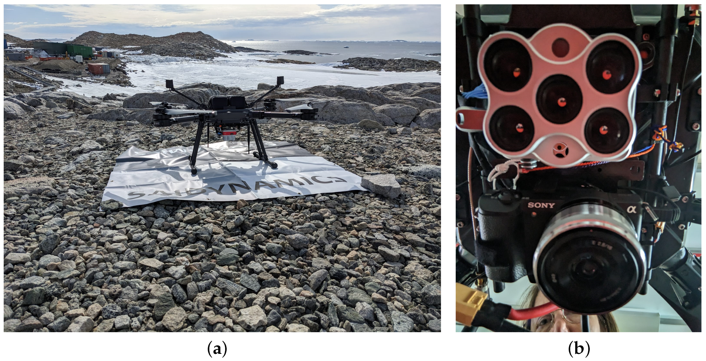
Remotesensing 15 05658 g002
Figure 3. UAV and sensors for aerial data collection in ASPA 135. (a) BMR3.9RTK UAV developed by SaiDynamics Australia. (b) MicaSense Altum multispectral (top), and Sony Alpha 5100 high-resolution RGB cameras mounted on the BMR3.9RTK.
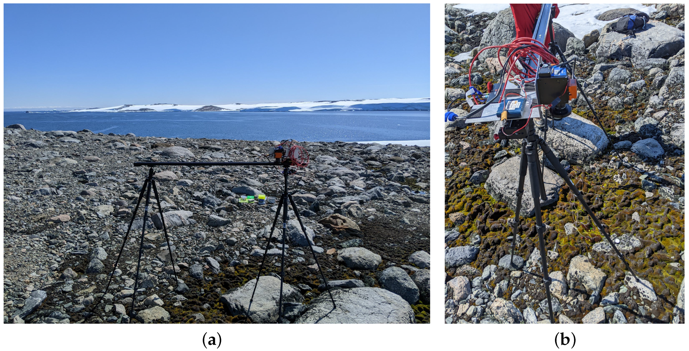
Remotesensing 15 05658 g003
Figure 4. Ground setup to collect HSI data in ASPA 135. (a) Careful placement of a Konova slider mounted to a pair of tripods on top of rocks to collect scans above fragile vegetation. (b) Side view of the ground setup, featuring a Headwall Hyperspec Nano hyperspectral camera pointing to the ground.
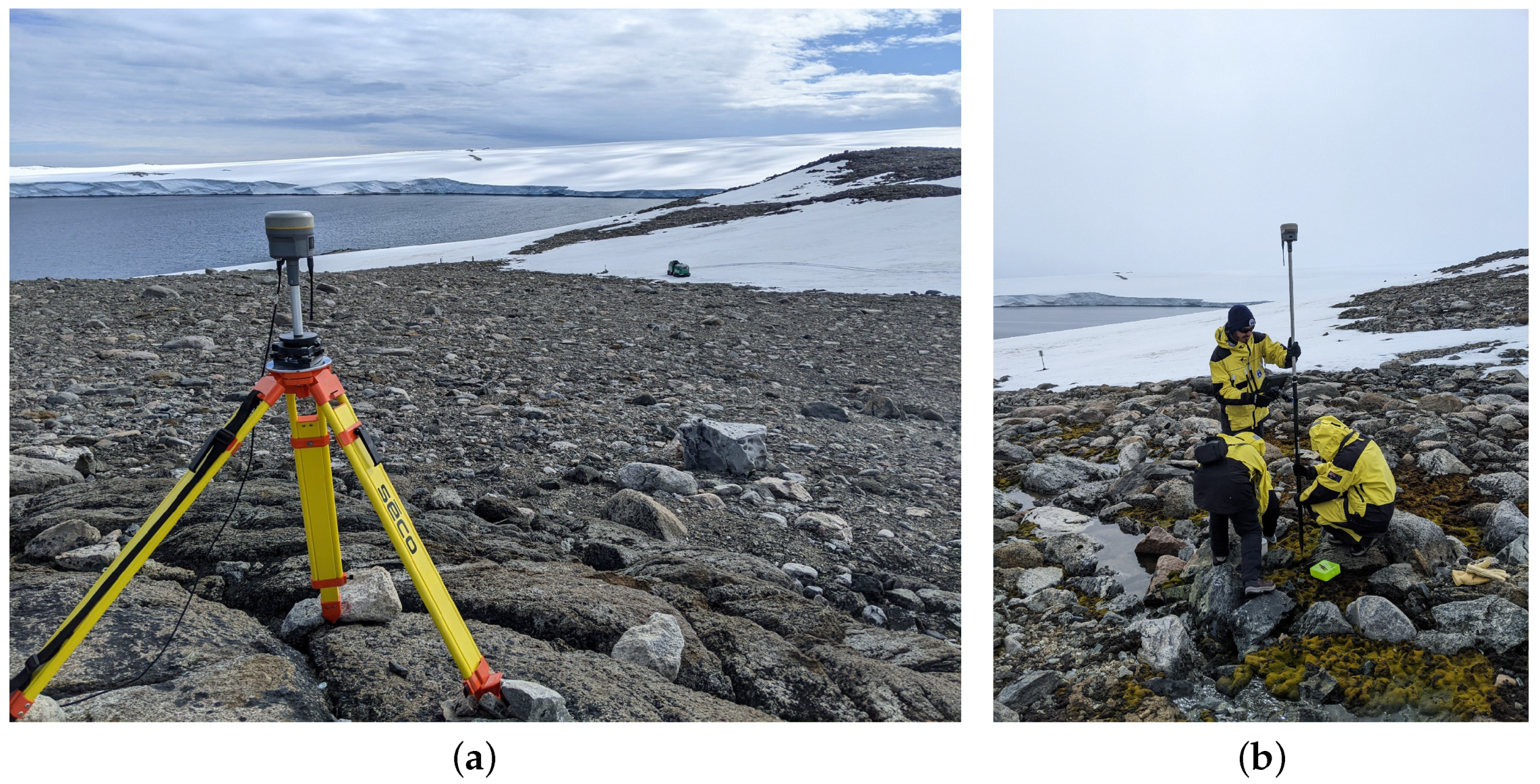
Remotesensing 15 05658 g004
Figure 5. Setup to collect GNSS points using a Trimble GNSS kit. (a) Base setup using a Trimble R10 antenna placed in a fixed marker with known GNSS coordinates. (b) Rover setup using a Trimble R10 antenna for precise GNSS RTK data collection, observing how expeditioners ensured the “no-step” rule over fragile vegetation.
Remotesensing 15 05658 g005
Figure 6. Alignment example between collected MSI and HSI data in ASPA 135. (a) Georeferenced MSI orthomosaic covering half of ASPA 135 boundaries (in purple), highlighting the area of interest where HSI scans took place (bright green) and historical locations of moss beds (orange dots). (b) Zoomed-in preview of (a), showing resulting HSI scans aligned with the MSI raster. The orange dots illustrate GNSS coordinates of historical quadrat locations of moss beds. (c) Zoomed-in preview of (b), depicting three HSI scans, providing high spectral and spatial resolutions of studied moss beds.
Remotesensing 15 05658 g006aRemotesensing 15 05658 g006b
Figure 7. Illustration of the training sample collection process from an HSI scan. (a) RGB preview of a sample HSI scan displaying a portion of a moss bed that contains the three health classifications, black lichen, bare rocks, ice, plastic, the spectralon (white circle in the middle), and metal from the tripod legs. (b) Polygons highlighting homogeneous areas corresponding to each one of the five classes.
Remotesensing 15 05658 g007
Figure 8. Plot of the average spectral signatures for each class reveals the unique patterns of light absorption and reflection. These spectral signatures are used to identify specific wavelength bands for discriminating between moss and lichen classes.
Remotesensing 15 05658 g008
Figure 9. Correlation heatmap illustrating the relationships between moss health ratings and various vegetation indices and statistical features.
Remotesensing 15 05658 g009
Figure 10. Bar diagram of feature ranking, displaying the importance of different features in the model’s prediction. The importance scores represent the contribution of each feature, with higher scores indicating higher importance. (a) Model 1 (all features, including spectral bands). (b) Model 3 (only derivative features).
Remotesensing 15 05658 g010aRemotesensing 15 05658 g010b
Figure 11. Accuracy analysis after fitting ML models with a selected number of reduced ranked features. (a) Accuracy plot of Model 1, which contains all the features. (b) Accuracy plot of Model 3, which contains only derivative features.
Remotesensing 15 05658 g011
Figure 12. Comparison of predictions from an HSI scan (a) among (b) Model 1; (c) Model 2; (d) Model 3; and (e) Model 4. The optimised models (Models 3 and 4) showcase comparable performance to the full-feature models, with reduced computational demands.
Remotesensing 15 05658 g012
Figure 13. Examples of final output maps using the proposed workflow. (a) Hyperspectral scans overlaid on georeferenced background maps. (b) Corresponding prediction maps of moss health at historical moss quadrats at ASPA 135.
Remotesensing 15 05658 g013
Table 1. Total of labelled hyperspectral pixels per class using 11 HSI scans.
ClassNameLabelled Pixels
1Moss (healthy)14,060
2Moss (stressed)12,914
3Moss (moribund)17,549
4Lichen (black)7972
5Non-vegetated56,976
 Total109,471
Table 2. List of 21 established vegetation indices to classify moss health and lichen.
CategoryNameCategoryName
VegetationNormalised Difference Vegetation Index (NDVI) [38]Chlorophyll
and Pigment
Carotenoid Reflectance Index 1 (CRI1) [39]
Green Normalised Difference Vegetation Index (GNDVI) [40]Carotenoid Reflectance Index 2 (CRI2) [39]
Modified Soil Adjusted Vegetation Index (MSAVI) [41]Photochemical Reflectance Index (PRI) [42]
Enhanced Vegetation Index (EVI) [43]Red–Green Ratio Index (RGRI) [44]
Mean Red Edge (MRE) [45]Modified Chlorophyll Absorption Ratio Index (MCARI) [46]
Simple Ratio Index (SRI) [47]Stress
and Disease
Atmospherically Resistant Vegetation Index (ARVI) [48]
Normalised Difference Red Edge (NDRE) [45]Modified Red-Edge Simple Ratio (MRESR) [49]
Green Leaf Index (GLI) [50]OtherTriangular Vegetation Index (TVI) [51]
Water
Content
  Normalised Difference Water Index (NDWI) [52]Transformed Chlorophyll Absorption Reflectance Index (TCARI) [53]
Water Band Index (WBI) [54]Anthocyanin Reflectance Index 2 (ARI2) [55]
Excess Green (ExG) [56]
Table 3. List of new indices proposed in this study to aid and highlight spectral responses among stages of moss health and lichen classes.
NameEquationNameEquation
Normalized Difference Lichen Index (NDLI)
NDLI = B green B red B green + B red
Moss Triple Health Index (MTHI)
MTHI = B 888 · B 740 · B 560 B 678 · B 655 · B 490
Healthy–Moribund Moss Index (HMMI)
HMMI = B 860 B 678 B 860 + B 678
Inverse Moss Health Index (IMHI)
IMHI = B 490 B 860 B 688 B 720
Healthy–Stressed Moss Index (HSMI)
HSMI = B 740 B 655 B 740 + B 655
Normalised Difference Moss–Lichen Index (NDMLI)
NDMLI = B 920 B 480 B 480 + B 920
Stressed–Moribund Moss Index (SMMI)
SMMI = B 888 B 678 B 888 + B 678
Table 4. Comparison among the four tested models with total input features.
ModelDescription and Model InputInput Features
1A classifier incorporating over 200 reflectance bands from HSI scans, plus spectral indices, and statistical features.288
2An optimised version of Model 1, where feature selection techniques are applied to choose the best features from the original set.79
3A classifier that uses derivative features only, including spectral indices and statistical features.32
4An optimised instance of Model 3, employing feature selection to pinpoint the best derivative features for classification.23
Table 5. Comparison between prediction, recall, and F-score results per feature class of the four proposed ML models.
ClassMetricModel 1Model 2Model 3Model 4
Moss (healthy)Precision0.991.000.990.99
Recall1.001.001.000.99
F1-score1.001.001.000.99
Moss (stressed)Precision1.000.981.000.97
Recall0.980.990.980.98
F1-score0.990.980.990.98
Moss (moribund)Precision0.980.960.970.94
Recall0.980.980.980.97
F1-score0.980.970.980.96
Lichen (black)Precision0.920.910.910.90
Recall0.920.720.900.69
F1-score0.920.800.910.78
Non-vegetatedPrecision0.990.970.990.97
Recall0.990.980.990.98
F1-score0.990.980.990.97
Table 6. Macro and weighted average values of the four proposed ML models.
MetricAverageModel 1Model 2Model 3Model 4SupportClass
PrecisionMacro0.980.960.970.9533221
Weighted0.970.930.970.9224852
RecallMacro0.970.950.970.9444053
Weighted0.980.970.980.9614654
F1-scoreMacro0.980.970.980.9615,2395
Weighted0.980.970.980.96
Accuracy0.980.970.980.9626,916Total
Table 7. Mean accuracy and mean standard deviation values for Model 1 and Model 3 after applying k-fold cross-validation using ten folds.
ModelMean AccuracyMean Standard Deviation
Model 10.950.017
Model 30.950.009
Table 8. Confusion matrix of the five feature classes, showing excellent performance in predicting the correct classes with only a few misclassifications.
ClassModelMoss (Healthy)Moss (Stressed)Moss (Moribund)Lichen (Black)Non-Vegetated
Moss (healthy)133181003
233128002
333211000
4330418000
Moss (stressed)11724402008
21424611000
31624471903
42424412000
Moss (moribund)1144309289
22474297158
3164315974
43504287461
Lichen (black)10020135095
200281048389
300311325109
400331011421
Non-vegetated1204611515,076
2021569814,983
3106812515,045
40620411414,915
Disclaimer/Publisher’s Note: The statements, opinions and data contained in all publications are solely those of the individual author(s) and contributor(s) and not of MDPI and/or the editor(s). MDPI and/or the editor(s) disclaim responsibility for any injury to people or property resulting from any ideas, methods, instructions or products referred to in the content.

