


MSISR-STF: Spatiotemporal Fusion via Multilevel Single-Image Super-Resolution
by
 ,
,
Xiongwei Zheng
1,2,
Ruyi Feng
1,3,
Junqing Fan
1,3,
Wei Han
1,3,
Shengnan Yu
1,3 and
Jia Chen
1,3,* 1
School of Computer Science, China University of Geoscience, Wuhan 430074, China
2
China Geological Survey, Beijing 100037, China
3
Hubei Key Laboratory of Intelligent Geo-Information Processing, China University of Geosciences, Wuhan 430074, China
*
Author to whom correspondence should be addressed.
Remote Sens. 2023, 15(24), 5675; https://doi.org/10.3390/rs15245675
Submission received: 21 September 2023
/
Revised: 28 November 2023
/
Accepted: 5 December 2023
/
Published: 8 December 2023
(This article belongs to the Special Issue Advances and Challenges on Multisource Remote Sensing Image Fusion: Datasets, New Technologies, and Applications)
Abstract
:Due to technological limitations and budget constraints, spatiotemporal image fusion uses the complementarity of high temporal–low spatial resolution (HTLS) and high spatial–low temporal resolution (HSLT) data to obtain high temporal and spatial resolution (HTHS) fusion data, which can effectively satisfy the demand for HTHS data. However, some existing spatiotemporal image fusion models ignore the large difference in spatial resolution, which yields worse results for spatial information under the same conditions. Based on the flexible spatiotemporal data fusion (FSDAF) framework, this paper proposes a multilevel single-image super-resolution (SISR) method to solve this issue under the large difference in spatial resolution. The following are the advantages of the proposed method. First, multilevel super-resolution (SR) can effectively avoid the limitation of a single SR method for a large spatial resolution difference. In addition, the issue of noise accumulation caused by multilevel SR can be alleviated by learning-based SR (the cross-scale internal graph neural network (IGNN)) and then interpolation-based SR (the thin plate spline (TPS)). Finally, we add the reference information to the super-resolution, which can effectively control the noise generation. This method has been subjected to comprehensive experimentation using two authentic datasets, affirming that our proposed method surpasses the current state-of-the-art spatiotemporal image fusion methodologies in terms of performance and effectiveness.
1. Introduction
There has been a growing focus on dense time-series satellite data and high-resolution spatial imagery. An expanding array of applications is now demanding high temporal and high spatial resolution (HTHS) imagery, particularly for tasks, such as land use/cover mapping, change detection, and monitoring ecosystem dynamics. However, owing to technological constraints and budget limitations, various satellite sensors exhibit distinct temporal and spatial characteristics. Moreover, the desired HTHS data cannot be obtained. Many satellite designs are tailored to specific application requirements. For instance, certain remote sensing satellites, such as CBERS, SPOT5, and Landsat, are configured to provide a high spatial and low temporal (HSLT) resolution [1,2,3]. Their spatial resolution ranges from 5 to 30 m (SPOT5: 5 m; CBERS: m; and Landsat: 30 m). Nonetheless, achieving a higher spatial resolution often comes at the cost of longer revisit cycles, as seen in satellites, like SPOT5 (revisit cycle: 26 days), CBERS (revisit cycle: 26 days), and Landsat (revisit cycle: 15 days). In contrast, other satellites such as MODIS (revisit cycle: 2 days), AVHRR (revisit cycle: 6 days), and SPOT-VGT (revisit cycle: 1 day) are configured to provide a high temporal and low spatial (HTLS) resolution, thanks to their shorter revisit cycles [4,5]. Correspondingly, their spatial resolution ranges from 500 to 1200 m (MODIS: 500m; AVHRR: km; and SPOT-VGT: km). Hence, employing spatiotemporal image fusion technology to acquire HTHS images holds substantial significance.
Spatiotemporal image fusion [6,7] utilizes the complementarity of HTLS and HSLT data to obtain HTHS fusion data, which can effectively satisfy the demand for HTHS data. The key to solving the issue of spatiotemporal fusion is how to construct the corresponding relationship between each pair of HTLS-HSLT images simultaneously. At present, most algorithms focus on how to establish the corresponding relationship to build an algorithm model. The methodologies in this domain can be broadly categorized into five distinct groups [8]: weight-based, unmixing-based, Bayesian-based, learning-based, and hybrid methods. Weight-based methods [9,10,11,12,13,14,15] resample an HTLS image in the same size as that of an HSLT image to establish the spatial correspondence. Then, the weight is used to calculate the information variation to obtain an HTHS image. For example, the classical weight-based method is the Spatial and Temporal Adaptive Reflectance Fusion Model (STARFM) algorithm [9], which assumes that a reflectance change is linearly interpolated between the high-throughput high temporal–low spatial (HTLS) and high spatial–low temporal (HSLT) images when an HTLS pixel exclusively represents a single land cover type. In such cases, the high temporal–high spatial (HTHS) image can be straightforwardly derived by incorporating the change information. However, when an HTLS pixel encompasses multiple land cover types, STARFM employs a weighted approach by considering various factors from the neighboring HSLT pixels to generate the HTHS image. Unmixing-based methods [16,17,18,19,20,21,22,23,24] elucidate spatial correspondence by considering the perspective of mixed pixels, wherein each pixel in the HTLS image is regarded as a combination of pixels from the HSLT image. The spatial–temporal data fusion approach (STDFA) [19] is valid for cases where the temporal variations in the land cover types are constant, which calculates the changes in the land cover types between these two HTLS images and integrates them into the HSLT image. Bayesian-based methods [25,26,27,28,29] describe the spatial correspondence from the probability theory and regard the fusion problem as a maximum posterior problem for solving the optimal state with known observations. Hence, the pivotal aspect of this method lies in establishing the probability-based definition of the relationship between the input HTLS and HSLT images and the HTLS images. These relationships encompass covariance functions, as employed in [25], low-pass filtering as presented in [26], and joint covariance as detailed in [29]. Learning-based methods [30,31,32,33,34,35,36,37,38] consider that HTLS and HSLT images have the same or similar feature attributes in the spatial relationship. Learning-based methods extract image features through the process of learning and subsequently generate HTHS images by predicting HTLS images during the fusion phase. Currently, the dominant branches of the learning-based methods encompass dictionary learning, machine learning, and deep learning. The GAN-based spatiotemporal fusion model (GAN-STFM) [37] introduces the conditional generative adversarial network (CGAN) and switchable normalization technique into the spatiotemporal fusion problem. Hybrid methods [39,40,41,42,43,44,45] combine the advantages of the abovementioned methods to obtain better fusion accuracy. The robust flexible spatiotemporal data fusion (RFSDAF) [38] method uses a multiscale fusion strategy that is adaptive to different degrees of coregistration error. It incorporates multiscale information, which extends the analysis of the reflectance and class fraction from per-MODIS pixel to inter-MODIS pixels, and it is robust to coregistration errors. A rigorously incremental spatiotemporal data fusion method for fusing remote sensing images with different resolutions [45] utilizes the particle swarm optimization Gaussian mixture model to extract endmembers and establishes a linear relationship between sensors to obtain accurate time increments. Furthermore, bicubic interpolation is used instead of thin plate spline interpolation for spatial interpolation, and support vector regression is also used to calculate weights for obtaining a weighted sum of temporal and spatial increments. However, most solutions to the spatial correspondence of these methods are only suitable for applications where the spatial resolution difference is small, such as 4 times or 8 times.
As is known, the current demand for remote sensing data is such that what we get is not what we want. However, certain applications require spatiotemporal fusion under large spatial differences. If the spatial resolution difference is larger, such as 16 times or more, it may lead to a worse fusion result or the solution might not meet this condition. For example, with large differences in spatial resolution, the resampling of weight-based methods will face a situation where a pixel value is resampled into hundreds of values. Similarly, unmixing-based methods need to deal with a situation where one pixel is mixed with hundreds of pixels. The difference in the amount of spatial information can inevitably lead to errors in the fusion results. Bayesian-based methods need to deal with the lack of prior knowledge caused by differences in the spatial resolution. For learning-based methods, large differences in the spatial resolution can result in some HTLS image features that cannot be extracted due to a lack of information.
Hence, this paper’s primary focus lies in addressing spatiotemporal fusion challenges when dealing with substantial variations in spatial resolution. The most immediate consequence of such disparities in spatial resolution is the acquisition and incorporation of spatial information within the context of spatiotemporal fusion. To avoid mutual interference between temporal and spatial domain information, this article draws inspiration from the classic hybrid algorithm FSDAF. This model first predicts the change information from the temporal and spatial domains, separately. Then, the actual change information by weight is calculated to obtain the fusion result.
The spatial domain information is predicted to obtain images with more spatial information by enhancing the spatial details of HTLS images. SISR methods are generally used to solve this issue. SISR can be classified into learning-based [46,47,48,49,50] and interpolation-based SISR methods [51]. The advantage of learning-based methods is that they can learn the image features through training and then supplement the image details through the learned prior knowledge. In contrast, interpolation-based methods aim to supplement the image pixels through certain interpolation constraints.
In practice, a single SISR method typically achieves an optimal spatial resolution enhancement of 4 to 8 times. However, this falls short when dealing with SISR tasks requiring a resolution difference of 16 times or more, which is the specific focus of our study. To tackle the challenge of obtaining spatial resolution information at significantly larger scales, this paper proposes a multilevel SISR strategy. Our approach includes two processes. First, when there is less noise, we utilize a learning-based SISR method, IGNN, to extract the spatial features of an HTLS image. After the first step, as noise accumulates to a predetermined threshold, we employ an interpolation-based method, TPS, to mitigate the adverse impacts of excessive noise and supplement the image details. Therefore, our method combines the advantages of the two types of SISR methods to overcome the difficulty with a resolution difference of 16 times or more. In addition, we introduce more control information in the SISR process to ensure the transmission and integrity of the information in the multilevel SISR process.
The principal innovation presented in this methodology is the application of multilevel SISR for the generation of spatial information predictions within spatiotemproal fusion. Consequently, we refer to this approach as MSISR-STF in this paper.
The contribution of this work can be summarized as follows:
- 1.
- The multilevel SISR strategy can effectively solve spatiotemporal fusion with large differences in the spatial resolution.
- 2.
- IGNN uses similar blocks in the image to complete the details, which introduces more spatial information for spatiotemporal fusion.
- 3.
- MSISR-STF introduces more spatial information through constraint methods to improve the fusion accuracy.
The remainder of this paper is structured as follows: Section 2 provides a comprehensive overview of the problem definitions and variable descriptions. Section 3 presents detailed exposition of our proposed method, MSISR-STF, along with the primary flowchart illustrating its functionality. Section 4 presents the experimental setup and showcases the obtained results. The conclusion is drawn in Section 6.
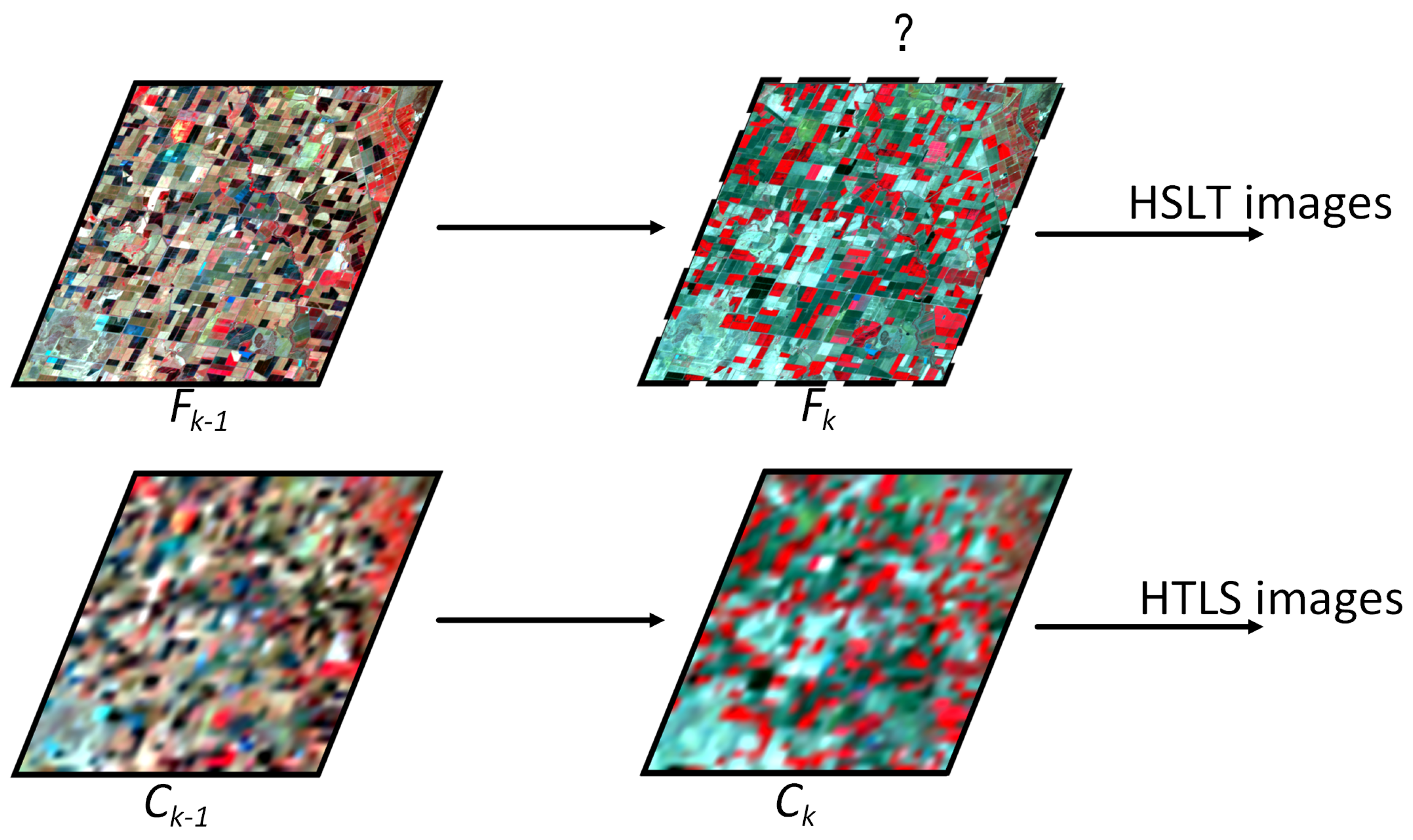
2. Problem Definition
In this paper, for the task of remote sensing image fusion, all images must be accurately matched in a unique geographic location. Registration must be calibrated between HTLS and HSLT images for fine geographic calibration. This problem is illustrated as Figure 1.
The following images are used in this spatiotemporal fusion:
- 1.
- A pair of an HSLT image and HTLS image at time .
- 2.
- An HTLS image at time k.
The unknown image that needs to be estimated is the HTHS image at time k.
In addition, the symbols used in this paper are defined in Table 1.
3. MSISR-STF
To solve the large differences in the spatial resolution for spatiotemporal image fusion, a multilevel SISR method is proposed to improve the spatial information by combining the advantages of the two types of reconstruction methods. The main flowchart of the proposed method is shown in Figure 2.
This section introduces our algorithm from the following four main perspectives.
- 1.
- We show the fusion framework used for the research goal, as well as its advantages.
- 2.
- For the prediction of spatial information under a large spatial resolution difference, we introduce a multilevel SISR strategy and introduce the constraint information to enhance this strategy.
- 3.
- For predicting temporal domain information, we use an unmixing-based method to solve the time-varying information.
- 4.
- We calculate the actual change, which is calculated by calculating the weight of the real change by using the amount of change in the predicted image in the temporal and spatial domains. The neighborhood pixels are used to enhance the robustness of the algorithm and fusion accuracy.
3.1. Fusion Framework
This research is primarily centered around the challenge of spatiotemporal fusion when confronted with substantial disparities in the spatial resolution. One of the immediate consequences of these spatial resolution differences is their impact on the acquisition and integration of spatial information within the context of spatiotemporal fusion. To avoid mutual interference between temporal domain information and spatial domain information, this article draws inspiration from the classic hybrid algorithm FSDAF. This model first obtains the prediction of the change information from the temporal and spatial domain separately and then calculates the actual change information by weight to obtain the fusion result.
In the design of the FSDAF model, there are two types of relationships in spatiotemporal fusion. One is the relationship between the observed HSLT and HTLS images observed on the same date in the spatial domain; this relationship is called the spatial model. The other is the relationship between the HSLT and HTLS images observed on different dates; this is called the temporal model. The scale model contains knowledge of the point spread function, which maps the pixels of an HSLT image to the corresponding HTLS image. The temporal model describes dynamic changes in the land surface, including changes in vegetation (such as seasonal changes) and sudden land cover changes (such as forest fires and floods). That is, how to accurately establish the scale model of time and space fusion and the time model is the key to solving the problem of spatiotemporal fusion.
Generally, spatiotemporal fusion can be expressed as the image to be solved, which is the sum of the image at the previous moment and the change in the information amount in this period.
where represents the difference between two HSLT images at and k. However, cannot be solved directly. In fact, the change information is concentrated in that of the HTLS images. Thus, Equation (1) can be written as follows:
where represents the relationship between the degradation of the HSLT and HTLS images and is related to the spatial model. In addition, represents the difference between two HTLS images at and k and is related to the temporal model. Considering the influence of the spatial and temporal model, the spatiotemporal fusion framework can be described as follows:
where represents the amount of information change under the influence of on the spatial scale, represents the amount of information change under the influence of on the temporal scale, and w represents the weight of . If and are used to represent the prediction based on the spatial and temporal domain, respectively, then
The variable in represents the scale model, which represents the difference in the spatial information, so can be equivalent to the difference after the spatial image prediction at k. The variable in represents the temporal model, which represents the difference in the temporal information, so can be equivalent to the difference after the spatial image prediction at k.
3.2. Prediction Based on the Spatial Domain
The spatial information prediction of spatiotemporal fusion is embodied in the spatial model. In general, the best approach to solving spatial models is SISR. However, the spatial resolution scale range of the current SISR methods ranges from 4 to 8 times, which does not meet the scale range of 16 times or more required in this study.
In this section, we introduce a multilevel SISR method to address the large-scale differences in spatial resolution. In addition, we present some issues faced in using the multilevel SISR method and our solutions to these problems.
- 1.
- Aiming at noise accumulation in multilevel SISR, we propose the idea of using the learning-based SISR method IGNN first and, then, the interpolation-based SISR method TPS.
- 2.
- Aiming at obtaining the insufficient spatial information of the HTLS images under large spatial resolution differences, we introduce more information and constraints to ensure information gain and information transmission.
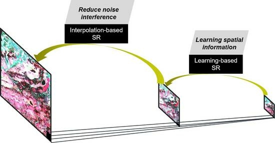
3.2.1. Noise Accumulation: IGNN + TPS
An inevitable issue that arises when using multilevel SISR is that the error caused by the first SISR gets amplified in the subsequent SISR. By comparing the current SISR methods, we consider the characteristics of the two types of SISR methods and propose to use the learning-based SISR method first and then the interpolation-based SISR method for spatial information prediction. First, a learning-based SISR method is used to train the feature correspondence between the HTLS-HSLT images, and the image resolution is enhanced on the basis of preserving the feature information of the image. Then, by using the smoothing function of an interpolation-based SISR method, the spatial information is enhanced without adding more errors. It is worth noting that the difference in the large-scale spatial resolution of this algorithm in this paper is 16 times. In addition, through a sensitivity analysis, the best multilevel SISR in this algorithm is the 4-times learning-based SISR method first, followed by the 4-times interpolation-based SISR method.
We use IGNN [52] as the first-level SISR method. Combined with graph convolution, IGNN proposes a non-local graph convolution aggregation module (GraphAgg). GraphAgg finds the k nearest neighbors (NNs) of the HSLT image blocks for each HTLS image block, constructs an HSLT-HTLS connection graph, and then aggregates the texture information of k HSLT image blocks corresponding to the HTLS image block to help the SISR.
The network uses an enhanced deep residual network for single-image super-resolution (EDSR) [47] as the backbone network and inserts the GraphAgg module into the middle of the EDSR for cross-scale high-definition block aggregation, as shown in Figure 3.
The aggregated high-definition features can be directly transferred to the back high-scale network layer through a cross-scale connection so that the network can directly perceive the high-definition texture hidden in the image features. The module mainly includes two steps: graph construction and block aggregation. Graph construction aims to search k NN blocks that are similar to the target by using the k-NN method. However, unlike the same-scale k-NN search, the cross-scale k-NN search cannot match image blocks directly on the original image. To find the k NN blocks, IGNN first downsamples the original image. For each target (blue box in Figure 3) in the original image, it searches k NN blocks (yellow box in Figure 3) from the downsampled image by block matching. Then, the k NN blocks are mapped to the scale of the original image by scale mapping, and k NN blocks are obtained. The cross-scale association of the target and the k NN blocks is modeled using a graph. Each NN block is regarded as a vertex, and each edge represents the direct similarity between the target and k NN blocks. Based on the constructed graph, IGNN proposes an adaptive block aggregation method, which defines the aggregation weight of the edge according to the similarity between the target and NN blocks. In addition, inspired by Adaptive Instance Normalization (AdaIN) [53], IGNN proposes Adaptive Patch Normalization (AdaPN) for image blocks to align the low-frequency signals of the neighboring blocks and the target without changing the high-frequency texture information.
EDSR is based on a super-resolution residual network (SRResNet), which includes the convolution layer (Conv), rectified linear units layer (ReLU), and batch normalization layer (BN). The Conv layer is used for feature extraction; the ReLU layer performs the activation function; and the BN layer can simplify the training of a deeper network, accelerate convergence, and have some regularization effect, which can prevent the over-fitting of the model. In terms of SISR and image generation, BN does not perform well. With the addition of batch norm, the training speed becomes slow, unstable, and even divergent. Therefore, EDSR is optimized by deleting the BN layer to simplify the SRResNet architecture, train the network with an appropriate loss function, and optimize the model.
Please refer to the original paper [52] for the specific implementation details.
Using IGNN, we can obtain images with a resolution ranging from 1 to 4 times.
TPS is used as the second-level SISR method. A surface passing through all the control points is established by the TPS function, and the gradient change in all the points is minimized. In other words, the spline function of the thin plate fits the control point with the minimum curvature surface. Given N known points, the estimated value of the TPS function is obtained as follows:
where are scalar; is the band A of the point i; and is the distance between the interpolation point and the coordinate value of the control point. To solve Equation (7), three additional control conditions are introduced.
where
Using TPS, we can obtain images with a resolution ranging from 4 to 16 times.
3.2.2. Insufficient Spatial Information: Information Gain + Information Transmission
Another unavoidable issue in this study is the lack of information caused by the large difference in spatial resolution. To solve this issue, this algorithm gains information by searching similar blocks with IGNN. In addition, we use TPS to supplement and transfer the gain information. Apparently, the multilevel SISR method can realize the large-scale spatial information prediction. However, to match similar blocks, IGNN adds downsampling processing. The mixed pixels caused by downsampling affect the selection of similar blocks. In addition, under the downsampling resolution, different objects with the same spectrum can also affect the gained information.
To ensure the effectiveness of the gain information, we use a wavelet transform to reprocess the spatial prediction results after multilevel SISR.
Wavelet transform uses a series of wavelets of different scales to decompose the original function and thus obtain the coefficients of the original function in different scales. In digital image processing, continuous wavelets need to be discretized in a wavelet transform. A discrete wavelet transform is obtained by discretizing the scale and displacement of the continuous wavelet transform according to the second power. The discrete wavelet transform decomposes the image into corresponding low- and high-frequency signals through low- and high-pass filters. The low-frequency signal represents the frame information of the image, whereas the high-frequency signal represents the detailed information of an image.
We use the wavelet transform to extract the frame information of an HTLS image and detailed information of a multilevel SISR image . In addition, we use the inverse transform of the wavelet transform to fuse the detail information into the frame information to ensure the accuracy of the gained information.
Then, the improved spatial prediction can be described as follows:
3.3. Prediction Based on the Temporal Domain
The temporal information of the spatiotemporal fusion model is in the change in the HTLS images. We use the unmixing-based method to predict the temporal information. The unmixing-based method assumes that the abundance of mixed pixels does not change with time. This is acceptable under a large spatial resolution difference. The steps can be described as follows.
3.3.1. Endmember and Abundance
First, the pixels in the HSLT image are classified by ISODATA. The number of endmembers is determined according to the classification results. Second, the abundance of each class is calculated according to the corresponding relationship of the resolution in the HTLS-HSLT images at the k-1 moment. Suppose an HTLS pixel corresponds to m HSLT pixels and can be divided into l classes. In the classification result, if the cth class has pixels, the quantity denoted as abundance, represented by the variable A, can be formulated as follows:
3.3.2. Change in Temporal Domain:
In accordance with the assumption underlying the theory of linear mixing, the alteration in the temporal domain information within an HTLS pixel can be conceptualized as the cumulative effect of temporal domain information changes across all HSLT pixels contained within that HTLS pixel:
Equation (12) signifies the temporal domain change information within the HTLS image, and Equation (13) remains valid within the framework of the linear mixing theory assumption. Consequently, by amalgamating Equations (12) to (13), it becomes possible to estimate the temporal domain change for each class, denoted as .
3.3.3. Temporal Prediction:
By allocating the temporal domain information changes for each class to the image , we can derive a predicted image that is grounded in the temporal domain at the moment k.
3.4. Final Fusion
In the previous section, we obtained the spatial and temporal prediction separately. In accordance with Equations (4) and (5) of the fusion model, this section describes the weight w of different pixels in the spatial and temporal domain. w is used to obtain the actual value with both spatial and temporal domain changes. In addition, considering the influence of the neighborhood pixels, a method of collecting the neighborhood influential factors is used to further update the fusion results.
3.4.1. Temporal and Spatial Prediction Weight: w
In accordance with the theory of unmixing, it is plausible to view an HTLS pixel as a composite blend of the corresponding m HSLT pixels:
Within the heterogeneous region, the residual of the HTLS image’s heterogeneous area can be formulated as:
By consolidating Equations (12)–(16), the expressions for the residuals within the heterogeneous regions, denoted as , can be derived as follows:
In the homogeneous region, the spatial prediction generated by TPS can accurately represent the actual value of an HSLT image. The residual within the homogeneous region, denoted as , can be formulated as:
FSDAF ascertains the extent of the influence exerted by the temporal and spatial domain predictions on the resultant pixel values by computing the weighting factors associated with the residual distributions from both the heterogeneous region, denoted as , and the homogeneous region, denoted as .
where the variable assumes values within the range of 0 to 1. When the q-th pixel in the HSLT image corresponds to the same land cover type as the central HSLT image pixel , takes on the value of 1.
Equations (19)–(21) facilitate the reassignment of residuals by computing the weighting factors associated with both homogeneous and heterogeneous residuals.
The actual variations denoted as within an HSLT pixel, derived from the residual distribution, are computed as follows:
3.4.2. Image Fusion Using Neighborhood Information
In the context of data fusion, in order to mitigate the uncertainties in the ultimate predictions, FSDAF employs an approach reminiscent of STARFM and ESTARFM, which integrates the neighborhood information. The weighting of this neighborhood information is contingent upon the pixel-to-pixel distance, denoted as :
where w is the window size.
4. Experiments and Analysis
The experiments and analyses encompassed the following parts: Datasets: The study considered the datasets used for experimentation. Quantitative evaluation indicators and comparison methods: The research employed specific metrics for quantitative evaluation and made comparisons with other methods. Experimental results: The outcomes and findings of the experiments were presented and discussed. Computational costs: The computational resources and costs associated with the proposed method were examined and reported.
4.1. Datasets
This algorithm’s experimental dataset employs satellite data from Landsat-7 ETM+ and MODIS. The images are situated at approximately 54N and 104W. We utilized three pairs of Landsat-7 ETM+ and MODIS images for evaluation purposes. To create false-color compositions, we employed the red, green, and near-infrared (NIR) bands.
The experimental datasets are depicted in Figure 4. In the context of MSISR-STF, one pair of HSLT images (Landsat-7 ETM+) and HTLS images (MODIS) obtained on 24 May 2001 (referred to as time ), along with the HTLS image acquired on 11 July 2001 (referred to as time k), were employed to predict the HSLT image at time k. Then, the predicted image was compared with a real Landsat ETM+ image acquired at time for assessing the performance of MSISR-STF (we call this model 3→1, which uses Figure 4a,d,e to obtain Figure 4b). However, in some spatiotemporal fusion algorithms, an additional pair of HTLS-HSLT images at time is required as the input. For example, spatiotemporal fusion via CycleGAN-based image generation (CycleGAN-STF) (we call this model 5→1, which uses Figure 4a,d,e,c,f to obtain Figure 4b). In addition, the enlarged area A in Figure 4b is used for the first experimental dataset, and the enlarged area B is used for the second dataset.
The spatial resolution of the Landsat-7 ETM+ satellite data is 30 m, while that of the MODIS data is 500 m. To bridge the spatial resolution difference of 16 times, we resampled the MODIS data to 480 m. Before engaging in the spatiotemporal fusion process, preprocessing steps, which encompassed calibration and resampling, were applied to both the HTLS and HSLT images.
4.2. Quantitative Evaluating Indicators and Comparison Methods
To assess the fusion outcomes, we conducted a comparison with the reference data. Additionally, various evaluation metrics were employed to assess the experimental dataset.
The first evaluation indicator is the root mean square error (RMSE), employed to measure the discrepancy between the actual and fused values. The RMSE quantifies how much the predicted value deviates from the true value, with smaller RMSE values indicating closer proximity of the fused image to the actual value.
The second evaluation indicator is the correlation coefficient (CC), which quantifies the degree of linear correlation between the research variables. A higher CC value implies a closer alignment between the predicted and actual images. A CC value of 1 indicates a perfect linear relationship between the predicted and actual images.
The third evaluation indicator is the structural similarity (SSIM) [54], employed to assess the similarity of the overall structures between the fused and actual images. The SSIM value ranges from −1 to 1, with higher values indicating a superior fusion outcome.
The fourth evaluation indicator is the spectral angle mapper (SAM) [55], which quantifies the spectral dissimilarity in the fused image. A smaller SAM value signifies better preservation of the spectral information in the fused image.
These evaluation indicators are employed to assess the fusion accuracy of the fusion algorithm presented in this paper. Among them, the RMSE, CC, and SSIM primarily emphasize spatial details, while SAM places a greater emphasis on spectral fidelity.
To gauge the impact of MSISR-STF, we have chosen traditional spatiotemporal fusion algorithms for a comparative analysis.
STARFM is a classic weight-based method, and its technique of using weight to integrate neighboring pixel information to predict pixels plays an important role in MSISR-STF. STARFM is a 3→1 model.
FSDAF is a classic hybrid method. MSISR-STF draws lessons from the fusion framework of FSDAF using temporal and spatial domain prediction. MSISR-STF improves FSDAF under a large-scale spatial difference. FSDAF is a 3→1 model.
CycleGAN-STF is a hybrid approach. The reason why we use CycleGAN-STF in this paper is that both CycleGAN-STF and MSISR-STF are spatiotemporal fusion methods under large-scale spatial differences. CycleGAN-STF is a 5→1 model.
4.3. Experimental Results
We conducted two distinct sets of experiments to thoroughly explore the capabilities of our algorithms. The first set of experiments was primarily centered around areas exhibiting pronounced and intricate changes in heterogeneity. In contrast, the second set of experiments encompassed alterations in land cover but within the broader context of substantial heterogeneity modifications. This deliberate division allowed us to assess how our algorithms perform under varying degrees of complexity and heterogeneity in the landscape.
As we delve into the results presented in Table 2 and Table 3, it is noteworthy that the bold numbers highlight the best-performing outcomes among the numerous algorithms evaluated. These bold numbers serve as indicators of excellence, signifying which algorithm excelled in capturing and representing the changes within the given experimental conditions. The emphasis on these best outcomes provides valuable insights into the strengths and adaptability of our algorithms across different scenarios, guiding us toward more informed decision making in our research and application endeavors.
Each dataset for comparison consisted of a image extracted from a larger image. The remaining portions were utilized as the training data for IGNN. Additionally, to augment the volume of training data, various operations such as rotation and flipping were applied.
4.3.1. The First Experimental Results: Heterogeneity Changes
Figure 5 shows the experimental results of the first set of data. Figure 5a–c present the input data of the 3→1 model and Figure 5d presents the ground truth. From Figure 5b to Figure 5d, we can observe pronounced heterogeneity changes. We have magnified the prominent segment in the experimental findings. Figure 5e–h are the experimental results of TPS+TPS, IGNN+IGNN, TPS+IGNN, and MSISR-STF (IGNN+TPS). Figure 5i–l are the experimental results of the first group data of STARFM, FSDAF, CycleGAN-STF, and MSISR-STF, respectively.
In the enlarged area in Figure 5d–l, we select sub-blocks A and B for comparison. From the visual effect of sub-block A, the results of CycleGAN-STF and MSISR-STF were closer to the ground truth. However, due to the large difference in their spatial resolutions, STARFM and FSDAF obtain very little information of the heterogeneity change from the HTLS image shown in Figure 5c. The result simply attempts to approach the real value, but the performances of STARFM and FSDAF are not good. From the visual effect of sub-block B, MSISR-STF performs the best. The second best performer is CycleGAN-STF. Due to the same reason as that for sub-block A, the effect of STARFM and FSDAF are closer to the HSLT image shown in Figure 5b.
Based on our experimental results, we observed significant noise in the images when using both the IGNN+IGNN and TPS+TPS methods. This suggests that neither of these methods effectively suppressed noise and, in fact, led to the accumulation of noise during the super-resolution process, resulting in a noise iteration scenario. This noise issue has had a noticeable adverse impact on image quality.
In contrast, when we employed the TPS+IGNN method, we achieved relatively good visual results. However, there were still noticeable levels of noise present, which may have affected the final visual quality of the images. These noise-related challenges could potentially limit the effectiveness of super-resolution techniques in practical applications.
To address these issues, we introduced a novel method called MSISR-STF, which involves learning first and then interpolating to process images. What sets this method apart is its ability to effectively suppress noise and enhance image quality. Numerically, our approach showed significant improvements across various performance metrics, indicating its effectiveness in the context of super-resolution tasks.
Table 2 presents a comprehensive overview of the evaluation metrics derived from our initial set of experiments. This table serves as a valuable reference point for assessing the performance of the various methods under scrutiny.
Upon closer examination of the data, a notable trend emerges: both CycleGAN-STF and MSISR-STF exhibit significantly superior outcomes compared to their counterparts, STARFM and FSDAF. This observation underscores the efficacy of CycleGAN-STF and MSISR-STF in addressing the specific challenges posed by the experimental context.
What is particularly striking is that MSISR-STF consistently outperforms all other methods across each evaluation metric. This comprehensive dominance across the board highlights MSISR-STF’s versatility and adaptability, suggesting that it possesses a unique ability to produce desirable outcomes in a variety of scenarios. This could be attributed to its capacity to effectively learn and adapt to the underlying data distribution, making it a robust choice for a wide range of image translation and enhancement tasks.
4.3.2. The Second Experimental Results: Land Cover Changes
In Figure 6, we present the data and outcomes stemming from the second set of experiments. Upon closer examination in the zoomed-in section of Figure 6, we discern interesting trends within sub-block A and sub-block B. Sub-block A displays a noticeable inclination toward exhibiting heterogeneous changes, suggesting a more diverse alteration pattern. Conversely, sub-block B appears to lean toward alterations in land cover, implying a greater focus on land transformation processes.
In this set of experimental results, we can clearly observe that whether using the IGNN+IGNN or TPS+TPS methods, there is still a small amount of noise present in the image results. This phenomenon primarily arises from the inability of these two super-resolution methods to effectively suppress noise, leading to the gradual accumulation of noise during the super-resolution process, resulting in a noise iteration scenario. The presence of noise can potentially affect the clarity and quality of the images, which is a significant issue that cannot be overlooked in some applications.
However, at the same time, when employing the TPS+IGNN method, we achieve relatively satisfactory visual results. Nevertheless, this method does not excel in preserving spatial details, implying that some image details may be lost, especially in highly homogeneous regions.
Furthermore, we also observed that these three methods did not perform well in handling the homogeneity variations within sub-block A. This suggests that these methods face challenges when dealing with uneven or complex image regions, leading to a decrease in performance.
However, the MSISR-STF method that we introduced demonstrates significant improvements across all aspects. Whether evaluated from a visual perspective or based on numerical metrics, our method shows a notable enhancement. This indicates that the MSISR-STF method is more adept at handling noise, preserving details, and exhibiting greater robustness in the face of homogeneity variations.
In terms of the visual impact, it is noteworthy that the performance of sub-block B in the STARFM model appears to be the least favorable, as evidenced by Figure 6b. The resultant output from STARFM aligns more closely with the observations made in Figure 6b. This observation points to the limitations of the STARFM model in capturing the desired changes effectively.
On the other hand, sub-block B of the FSDAF model exhibits superior performance, albeit with some noticeable pixel blocks missing in this sub-block. This highlights FSDAF’s capability to generate meaningful changes in land cover, although there is room for improvement in pixel accuracy.
Furthermore, CycleGAN-STF demonstrates a commendable performance in sub-block B, outperforming MSISR-STF. This suggests that CycleGAN-STF excels in capturing and translating changes related to land cover in this specific context.
In terms of overall performance, sub-block A of MSISIR-STF emerges as the top performer, with FSDAF following closely behind. Notably, there exists a substantial disparity in the spectral characteristics between STARFM and CycleGAN-STF. This disparity emphasizes the distinct approaches taken by these models in capturing and representing changes in the landscape.
Table 3 displays the assessment metrics derived from this series of experiments, shedding light on the overall performance of the models under examination.
In a broad perspective, MSISR-STF demonstrates commendable results across all the evaluation indices, affirming its overall proficiency. However, it is noteworthy that in specific spectral bands, MSISR-STF lags behind the performance exhibited by both FSDAF and CycleGAN-STF. This underscores the notion that different models may exhibit varying strengths and weaknesses, which can be context-dependent and tied to specific spectral characteristics.
Interestingly, when evaluating the red band, FSDAF emerges as the frontrunner, registering the lowest root mean square error (RMSE). This signifies FSDAF’s exceptional accuracy in predicting changes within this particular band, making it a robust choice for tasks demanding precise quantitative assessments.
Conversely, CycleGAN-STF excels in the red band when assessing the correlation coefficient (CC) and the structural similarity index (SSIM). These superior values imply that CycleGAN-STF effectively captures and maintains both the correlation and structural fidelity between the generated and observed images within this band. This makes CycleGAN-STF particularly well suited for applications where preserving structural information is paramount.
However, it is important to note that the green band of MSISR-STF falls short when compared to FSDAF and CycleGAN-STF in terms of SSIM. This discrepancy hints at a potential challenge for MSISR-STF in maintaining image fidelity, especially within the green spectral band. Further refinement and optimization might be necessary to enhance its performance in this specific regard.
4.4. Computational Costs
The testing of this algorithm was carried out on a computer with the following specifications: Intel(R) Core(TM) i7-8700K CPU (3.70 GHz), 32 GB RAM, and a 3090 GPU. Table 4 shows the execution times under identical experimental settings. During the experiment, STARFM and FSDAF were implemented using ENVI IDE. CycleGAN-STF employed Python (Cycle-GAN), MATLAB (wavelet transform), and ENVI IDE (the fusion part). MSISR-STF utilized Python (IGNN), MATLAB (TPS), and ENVI IDE (the fusion part).
Because Cycle-GAN and IGNN necessitate the use of a GPU, we split the computational time costs into two components: training and fusion. We employed the GPU during the training phase and the CPU during the fusion phase, ensuring equitable time costs.
Table 4 demonstrates that CycleGAN-STF incurs the least computational time costs among all the algorithms in the fusion phase, followed by MSISR-STF. However, compared to the other two algorithms, CycleGAN-STF and IGNN require a more extended data training time. Specifically, each epoch takes 9 s for CycleGAN and 12 s for IGNN, with the epoch count set to 300 in the experimental data. Consequently, this results in a relatively longer total time cost for our algorithm. Nonetheless, in the actual fusion task, we perform thousands of fusion operations, whereas the training process only needs to be executed once. Therefore, the training time costs for the fusion task remain reasonable.
5. Discussions
This study employed a multilevel super-resolution approach to extract spatial information, aiming to maximize the retrieval and preservation of valuable details within low-resolution images through a process of learning followed by interpolation. The testing was conducted on two distinct datasets with distinctive characteristics, and the results indicate that our method achieved favorable outcomes, both visually and numerically, meeting the anticipated objectives. Furthermore, it successfully accomplished spatiotemporal fusion at a larger spatial resolution scale.
Our method adopts the idea of learning before interpolation and has been tested on existing datasets. We hope to learn more effective information from images through learning methods and then save the information through interpolation while enlarging the size. In addition, the other three methods all have theoretical flaws. Interpolation+Interpolation: The interpolation uses a smoothing function, which causes a large amount of information to be lost in each interpolation. If two interpolations are used, the image with limited useful information will only have a very small amount of information transmitted to the fused image. Learning+Learning: The learning method can effectively capture effective features. But, for two studies, first of all, training the dataset is a relatively large problem. This is because we need an intermediate resolution data for training. And our data are Landsat and MODIS data, which means that we need to learn twice and overcome the impact of sensor differences at least once during the training process. This can cause significant noise interference, resulting in poor results. Our test results also indicate this situation. Interpolation+Learning: The smoothing function of the interpolation can cause some information loss, and obtaining features from the interpolation results through learning methods cannot guarantee the accuracy of the learned features. In addition, the noise caused by the interpolation will also be learned by the learning method. So, our method ultimately chose the mode of learning before the interpolation. In addition, in order to overcome the shortcomings of two different methods, we have also added some control information ideas to minimize the interference of noise as much as possible.
However, this method still possesses certain limitations at present. Firstly, this type of approach tends to excel primarily in scenarios with significant differences in the large-scale spatial resolution. However, its performance may not be as prominent when dealing with small-scale spatial variations. Additionally, the method’s temporal scale prediction is relatively simplistic, and there is room for improvement in future work in this regard.
6. Conclusions
This paper presents a novel approach to address the challenge of handling significant disparities in spatial resolution in the context of spatiotemporal image fusion. Our proposed method, referred to as multilevel single-image super-resolution for spatiotemporal fusion (MSISR-STF), is designed to leverage the benefits of two distinct yet complementary techniques: super-resolution reconstruction based on learning and interpolation.
The motivation behind MSISR-STF lies in the inherent difficulties posed by large spatial resolution differences when attempting to fuse heterogeneous remote sensing data sources. In scenarios where data from high-resolution and low-resolution sensors need to be integrated, achieving seamless fusion becomes a formidable task. Traditional approaches often fall short in preserving the spatial details and spectral characteristics, especially when dealing with substantial resolution gaps.
MSISR-STF addresses this challenge by first learning the unique features and characteristics of low-resolution images. It extracts valuable information from these images using advanced learning techniques, enhancing their inherent spatial details. Subsequently, it leverages interpolation methods to upsample the low-resolution images, bridging the resolution gap to align them with high-resolution counterparts.
The experimental analysis conducted in this study confirms the effectiveness of our approach. The results indicate that by incorporating the knowledge acquired from low-resolution images before the interpolation step, MSISR-STF significantly mitigates the issues associated with large resolution disparities. This, in turn, leads to notable improvements in fusion accuracy.
Author Contributions
Data curation, X.Z.; Conceptualization, J.C. and X.Z.; Methodology, R.F., J.C. and X.Z.; Supervision, R.F., J.C. and J.F.; Writing—original draft, J.C. and X.Z.; writing—review and editing, S.Y., J.C. and X.Z.; formal analysis, S.Y. and W.H. All authors have read and agreed to the published version of the manuscript.
Funding
This work is funded by the National Natural Science Foundation of China (U1711266 and No. 41925007) and the Hong Kong Scholars Program (XJ2020025).
Data Availability Statement
No new data were created or analyzed in this study. Data sharing is not applicable to this article.
Conflicts of Interest
The authors declare no conflict of interest.
References
- Masek, J.G.; Huang, C.; Wolfe, R.; Cohen, W.; Hall, F.; Kutler, J.; Nelson, P. North American forest disturbance mapped from a decadal Landsat record. Remote Sens. Environ. 2008, 112, 2914–2926. [Google Scholar] [CrossRef]
- Brezini, S.; Deville, Y. Hyperspectral and Multispectral Image Fusion with Automated Extraction of Image-Based Endmember Bundles and Sparsity-Based Unmixing to Deal with Spectral Variability. Sensors 2023, 23, 2341. [Google Scholar] [CrossRef] [PubMed]
- Senf, C.; Leitão, P.J.; Pflugmacher, D.; van der Linden, S.; Hostert, P. Mapping land cover in complex Mediterranean landscapes using Landsat: Improved classification accuracies from integrating multi-seasonal and synthetic imagery. Remote Sens. Environ. 2015, 156, 527–536. [Google Scholar] [CrossRef]
- Vogelmann, J.E.; Howard, S.M.; Yang, L.; Larson, C.R.; Wylie, B.K.; Van Driel, N. Completion of the 1990s National Land Cover Data Set for the conterminous United States from Landsat Thematic Mapper data and ancillary data sources. Photogramm. Eng. Remote Sens. 2001, 67, 650–662. [Google Scholar]
- Dou, M.; Chen, J.; Chen, D.; Chen, X.; Deng, Z.; Zhang, X.; Xu, K.; Wang, J. Modeling and simulation for natural disaster contingency planning driven by high-resolution remote sensing images. Future Gener. Comput. Syst. 2014, 37, 367–377. [Google Scholar] [CrossRef]
- Gao, F.; Hilker, T.; Zhu, X.; Anderson, M.; Masek, J.; Wang, P.; Yang, Y. Fusing Landsat and MODIS data for vegetation monitoring. IEEE Geosci. Remote Sens. Mag. 2015, 3, 47–60. [Google Scholar] [CrossRef]
- Justice, C.; Townshend, J.; Vermote, E.; Masuoka, E.; Wolfe, R.; Saleous, N.; Roy, D.; Morisette, J. An overview of MODIS Land data processing and product status. Remote Sens. Environ. 2002, 83, 3–15. [Google Scholar] [CrossRef]
- Zhu, X.; Cai, F.; Tian, J.; Williams, T. Spatiotemporal fusion of multisource remote sensing data: Literature survey, taxonomy, principles, applications, and future directions. Remote Sens. 2018, 10, 527. [Google Scholar] [CrossRef]
- Gao, F.; Masek, J.; Schwaller, M.; Hall, F. On the blending of the Landsat and MODIS surface reflectance: Predicting daily Landsat surface reflectance. IEEE Trans. Geosci. Remote Sens. 2006, 44, 2207–2218. [Google Scholar]
- Hilker, T.; Wulder, M.A.; Coops, N.C.; Linke, J.; McDermid, G.; Masek, J.G.; Gao, F.; White, J.C. A new data fusion model for high spatial-and temporal-resolution mapping of forest disturbance based on Landsat and MODIS. Remote Sens. Environ. 2009, 113, 1613–1627. [Google Scholar] [CrossRef]
- Zhu, X.; Chen, J.; Gao, F.; Chen, X.; Masek, J.G. An enhanced spatial and temporal adaptive reflectance fusion model for complex heterogeneous regions. Remote Sens. Environ. 2010, 114, 2610–2623. [Google Scholar] [CrossRef]
- Fu, D.; Chen, B.; Wang, J.; Zhu, X.; Hilker, T. An improved image fusion approach based on enhanced spatial and temporal the adaptive reflectance fusion model. Remote Sens. 2013, 5, 6346–6360. [Google Scholar] [CrossRef]
- Wu, B.; Huang, B.; Cao, K.; Zhuo, G. Improving spatiotemporal reflectance fusion using image inpainting and steering kernel regression techniques. Int. J. Remote Sens. 2017, 38, 706–727. [Google Scholar] [CrossRef]
- Wang, Q.; Atkinson, P.M. Spatio-temporal fusion for daily Sentinel-2 images. Remote Sens. Environ. 2018, 204, 31–42. [Google Scholar] [CrossRef]
- Guo, D.; Shi, W.; Zhang, H.; Hao, M. A Flexible Object-Level Processing Strategy to Enhance the Weight Function-Based Spatiotemporal Fusion Method. IEEE Trans. Geosci. Remote Sens. 2022, 60, 1–11. [Google Scholar] [CrossRef]
- Li, H.; Feng, R.; Wang, L.; Zhong, Y.; Zhang, L. Superpixel-Based Reweighted Low-Rank and Total Variation Sparse Unmixing for Hyperspectral Remote Sensing Imagery. IEEE Trans. Geosci. Remote Sens. 2021, 59, 629–647. [Google Scholar] [CrossRef]
- Zhukov, B.; Oertel, D.; Lanzl, F.; Reinhäckel, G. Unmixing-based multisensor multiresolution image fusion. IEEE Trans. Geosci. Remote Sens. 1999, 37, 1212–1226. [Google Scholar] [CrossRef]
- Zurita-Milla, R.; Clevers, J.G.; Schaepman, M.E. Unmixing-based Landsat TM and MERIS FR data fusion. IEEE Geosci. Remote Sens. Lett. 2008, 5, 453–457. [Google Scholar] [CrossRef]
- Wu, M.; Niu, Z.; Wang, C.; Wu, C.; Wang, L. Use of MODIS and Landsat time series data to generate high-resolution temporal synthetic Landsat data using a spatial and temporal reflectance fusion model. J. Appl. Remote Sens. 2012, 6, 063507. [Google Scholar]
- Zhang, W.; Li, A.; Jin, H.; Bian, J.; Zhang, Z.; Lei, G.; Qin, Z.; Huang, C. An enhanced spatial and temporal data fusion model for fusing Landsat and MODIS surface reflectance to generate high temporal Landsat-like data. Remote Sens. 2013, 5, 5346–5368. [Google Scholar] [CrossRef]
- Wu, M.; Huang, W.; Niu, Z.; Wang, C. Generating daily synthetic Landsat imagery by combining Landsat and MODIS data. Sensors 2015, 15, 24002–24025. [Google Scholar] [CrossRef] [PubMed]
- Lu, M.; Chen, J.; Tang, H.; Rao, Y.; Yang, P.; Wu, W. Land cover change detection by integrating object-based data blending model of Landsat and MODIS. Remote Sens. Environ. 2016, 184, 374–386. [Google Scholar] [CrossRef]
- Jiang, X.; Huang, B. Unmixing-Based Spatiotemporal Image Fusion Accounting for Complex Land Cover Changes. IEEE Trans. Geosci. Remote Sens. 2022, 60, 1–10. [Google Scholar] [CrossRef]
- Zhou, J.; Sun, W.; Meng, X.; Yang, G.; Ren, K.; Peng, J. Generalized Linear Spectral Mixing Model for Spatial–Temporal–Spectral Fusion. IEEE Trans. Geosci. Remote Sens. 2022, 60, 1–16. [Google Scholar] [CrossRef]
- Li, A.; Bo, Y.; Zhu, Y.; Guo, P.; Bi, J.; He, Y. Blending multi-resolution satellite sea surface temperature (SST) products using Bayesian maximum entropy method. Remote Sens. Environ. 2013, 135, 52–63. [Google Scholar] [CrossRef]
- Huang, B.; Zhang, H.; Song, H.; Wang, J.; Song, C. Unified fusion of remote-sensing imagery: Generating simultaneously high-resolution synthetic spatial–temporal–spectral earth observations. Remote Sens. Lett. 2013, 4, 561–569. [Google Scholar] [CrossRef]
- Shen, H.; Meng, X.; Zhang, L. An integrated framework for the spatio-temporal-spectral fusion of remote sensing images. IEEE Trans. Geosci. Remote Sens. 2016, 54, 7135–7148. [Google Scholar] [CrossRef]
- Liao, L.; Song, J.; Wang, J.; Xiao, Z.; Wang, J. Bayesian method for building frequent Landsat-like NDVI datasets by integrating MODIS and Landsat NDVI. Remote Sens. 2016, 8, 452. [Google Scholar] [CrossRef]
- Xue, J.; Leung, Y.; Fung, T. A Bayesian data fusion approach to spatio-temporal fusion of remotely sensed images. Remote Sens. 2017, 9, 1310. [Google Scholar] [CrossRef]
- Liu, P.; Wang, L.; Ranjan, R.; He, G.; Zhao, L. A Survey on Active Deep Learning: From Model Driven to Data Driven. ACM Comput. Surv. 2022, 54, 221:1–221:34. [Google Scholar] [CrossRef]
- Huang, B.; Song, H. Spatiotemporal reflectance fusion via sparse representation. IEEE Trans. Geosci. Remote Sens. 2012, 50, 3707–3716. [Google Scholar] [CrossRef]
- Song, H.; Huang, B. Spatiotemporal satellite image fusion through one-pair image learning. IEEE Trans. Geosci. Remote Sens. 2012, 51, 1883–1896. [Google Scholar] [CrossRef]
- Li, L.; Liu, P.; Wu, J.; Wang, L.; He, G. Spatiotemporal Remote-Sensing Image Fusion With Patch-Group Compressed Sensing. IEEE Access 2020, 8, 209199–209211. [Google Scholar] [CrossRef]
- Tao, X.; Liang, S.; Wang, D.; He, T.; Huang, C. Improving satellite estimates of the fraction of absorbed photosynthetically active radiation through data integration: Methodology and validation. IEEE Trans. Geosci. Remote Sens. 2017, 56, 2107–2118. [Google Scholar] [CrossRef]
- Wei, J.; Wang, L.; Liu, P.; Song, W. Spatiotemporal fusion of remote sensing images with structural sparsity and semi-coupled dictionary learning. Remote Sens. 2016, 9, 21. [Google Scholar] [CrossRef]
- Song, H.; Liu, Q.; Wang, G.; Hang, R.; Huang, B. Spatiotemporal satellite image fusion using deep convolutional neural networks. IEEE J. Sel. Top. Appl. Earth Obs. Remote Sens. 2018, 11, 821–829. [Google Scholar] [CrossRef]
- Tan, Z.; Gao, M.; Li, X.; Jiang, L. A Flexible Reference-Insensitive Spatiotemporal Fusion Model for Remote Sensing Images Using Conditional Generative Adversarial Network. IEEE Trans. Geosci. Remote Sens. 2022, 60, 1–13. [Google Scholar] [CrossRef]
- Hou, S.; Sun, W.; Guo, B.; Li, X.; Zhang, J.; Xu, C.; Li, X.; Shao, Y.; Li, C. RFSDAF: A New Spatiotemporal Fusion Method Robust to Registration Errors. IEEE Trans. Geosci. Remote Sens. 2022, 60, 1–18. [Google Scholar] [CrossRef]
- Xu, Y.; Huang, B.; Xu, Y.; Cao, K.; Guo, C.; Meng, D. Spatial and temporal image fusion via regularized spatial unmixing. IEEE Geosci. Remote Sens. Lett. 2015, 12, 1362–1366. [Google Scholar]
- Gevaert, C.M.; García-Haro, F.J. A comparison of STARFM and an unmixing-based algorithm for Landsat and MODIS data fusion. Remote Sens. Environ. 2015, 156, 34–44. [Google Scholar] [CrossRef]
- Zhu, X.; Helmer, E.H.; Gao, F.; Liu, D.; Chen, J.; Lefsky, M.A. A flexible spatiotemporal method for fusing satellite images with different resolutions. Remote Sens. Environ. 2016, 172, 165–177. [Google Scholar] [CrossRef]
- Xie, D.; Zhang, J.; Zhu, X.; Pan, Y.; Liu, H.; Yuan, Z.; Yun, Y. An improved STARFM with help of an unmixing-based method to generate high spatial and temporal resolution remote sensing data in complex heterogeneous regions. Sensors 2016, 16, 207. [Google Scholar] [CrossRef] [PubMed]
- Li, X.; Ling, F.; Foody, G.M.; Ge, Y.; Zhang, Y.; Du, Y. Generating a series of fine spatial and temporal resolution land cover maps by fusing coarse spatial resolution remotely sensed images and fine spatial resolution land cover maps. Remote Sens. Environ. 2017, 196, 293–311. [Google Scholar] [CrossRef]
- Chen, J.; Wang, L.; Feng, R.; Liu, P.; Han, W.; Chen, X. CycleGAN-STF: Spatiotemporal Fusion via CycleGAN-Based Image Generation. IEEE Trans. Geosci. Remote Sens. 2020, 59, 5851–5865. [Google Scholar] [CrossRef]
- Jing, W.; Lou, T.; Wang, Z.; Zou, W.; Xu, Z.; Mohaisen, L.; Li, C.; Wang, J. A Rigorously-Incremental Spatiotemporal Data Fusion Method for Fusing Remote Sensing Images. IEEE J. Sel. Top. Appl. Earth Obs. Remote Sens. 2023, 16, 6723–6738. [Google Scholar] [CrossRef]
- Dong, C.; Loy, C.C.; He, K.; Tang, X. Image super-resolution using deep convolutional networks. IEEE Trans. Pattern Anal. Mach. Intell. 2015, 38, 295–307. [Google Scholar] [CrossRef]
- Lim, B.; Son, S.; Kim, H.; Nah, S.; Mu Lee, K. Enhanced deep residual networks for single image super-resolution. In Proceedings of the IEEE Conference on Computer Vision and Pattern Recognition Workshops, Honolulu, HI, USA, 21–26 July 2017; pp. 136–144. [Google Scholar]
- Xu, Y.; Wu, Z.; Chanussot, J.; Wei, Z. Hyperspectral Images Super-Resolution via Learning High-Order Coupled Tensor Ring Representation. IEEE Trans. Neural Netw. Learn. Syst. 2020, 11, 4747–4760. [Google Scholar] [CrossRef]
- Liu, Z.; Feng, R.; Wang, L.; Zeng, T. Gradient Prior Dilated Convolution Network for Remote Sensing Image Super-Resolution. IEEE J. Sel. Top. Appl. Earth Obs. Remote Sens. 2023, 16, 3945–3958. [Google Scholar] [CrossRef]
- Lin, Z.; Shum, H.Y. Fundamental limits of reconstruction-based superresolution algorithms under local translation. IEEE Trans. Pattern Anal. Mach. Intell. 2004, 26, 83–97. [Google Scholar]
- Bookstein, F.L. Principal warps: Thin-plate splines and the decomposition of deformations. IEEE Trans. Pattern Anal. Mach. Intell. 1989, 31, 567–585. [Google Scholar] [CrossRef]
- Zhou, S.; Zhang, J.; Zuo, W.; Loy, C.C. Cross-scale internal graph neural network for image super-resolution. Adv. Neural Inf. Process. Syst. 2020, 33, 3499–3509. [Google Scholar]
- Huang, X.; Belongie, S. Arbitrary Style Transfer in Real-Time with Adaptive Instance Normalization. In Proceedings of the 2017 IEEE International Conference on Computer Vision (ICCV), Venice, Italy, 22–29 October 2017; pp. 1510–1519. [Google Scholar]
- Wang, Z.; Bovik, A.C.; Sheikh, H.R.; Simoncelli, E.P. Image quality assessment: From error visibility to structural similarity. IEEE Trans. Image Process. 2004, 13, 600–612. [Google Scholar] [CrossRef] [PubMed]
- Yuhas, R.H.; Goetz, A.F.; Boardman, J.W. Discrimination among semi-arid landscape endmembers using the spectral angle mapper (SAM) algorithm. In Proceedings of the Summaries of the Third Annual JPL Airborne Geoscience Workshop, Pasadena, CA, USA, 1–5 June 1992; pp. 147–149. [Google Scholar]
Figure 1.
Problem definition. Given a pair of an HSLT image and HTLS image at time , the task is to estimate the unobserved HTHS image at time k.
Figure 1.
Problem definition. Given a pair of an HSLT image and HTLS image at time , the task is to estimate the unobserved HTHS image at time k.

Figure 2.
Flowchart of the algorithm model.

Figure 3.
Algorithm description of image prediction in spatial domain. We use IGNN and TPS as our multilevel SISR method.
Figure 3.
Algorithm description of image prediction in spatial domain. We use IGNN and TPS as our multilevel SISR method.

Figure 4.
Experimental data. (a,d) HSLT and HTLS image in , (b,e) HSLT and HTLS image in k, and (c,f) HSLT and HTLS image in . The enlarged area in (b) is the selected redtwo experimental data locations. The rest of the image is cropped as training data for IGNN when a set of experiments is conducted. (c,f) are used to serve FSDAF as another set of HSLT and HTLS data.

Figure 5.
The first set of experimental result. (a) HTLS image in , (b) HSLT image in , (c) HTLS image in k, (d) HSLT image in k, (e) TPS+TPS, (f) IGNN+IGNN, (g) TPS+IGNN, (h) MSISR-STF, (i) STARFM, (j) FSDAF, (k) CycleGAN-STF, and (l) MSISR-STF. Sub-block A and Sub-block B exhibit a clear inclination towards manifesting heterogeneous changes.

Figure 6.
The second set of experimental result. (a) HTLS image in , (b) HSLT image in , (c) HTLS image in k, (d) HSLT image in k, (e) TPS+TPS, (f) IGNN+IGNN, (g) TPS+IGNN, (h) MSISR-STF, (i) STARFM, (j) FSDAF, (k) CycleGAN-STF, and (l) MSISR-STF. Sub-block A exhibits a clear inclination towards manifesting heterogeneous changes, sub-block B appears to favor alterations in land cover changes.


Table 1.
Definitions of symbols used in this paper.
| Symbol | Definition |
|---|---|
| k | k refers to time, where , k, and represent the past time, the fusion time, and the future time in this paper, respectively. |
| i, j | The ith HTLS image pixel is denoted by i, and the jth HSLT image pixel in one HTLS image pixel is denoted by j. |
| The coordinate values of the ith HTLS image pixel. | |
| The coordinate values of the jth HSLT pixel in the HTLS pixel at location . | |
| C is the HTLS image and F is the HSLT image. | |
| The position of k refers to time. | |
| The cth class. |
Table 2.
The first set of experimental result.
| Method | RMSE | CC | SSIM | SAM | |||||||||
|---|---|---|---|---|---|---|---|---|---|---|---|---|---|
| Red | Green | NIR | All | Red | Green | NIR | All | Red | Green | NIR | All | ||
| TPS + TPS | 0.142 | 0.161 | 0.171 | 0.166 | 0.853 | 0.873 | 0.813 | 0.866 | 0.882 | 0.734 | 0.835 | 0.825 | 0.042 |
| IGNN + IGNN | 0.127 | 0.154 | 0.178 | 0.157 | 0.891 | 0.866 | 0.806 | 0.862 | 0.906 | 0.785 | 0.863 | 0.853 | 0.036 |
| TPS + IGNN | 0.143 | 0.157 | 0.132 | 0.142 | 0.923 | 0.893 | 0.843 | 0.873 | 0.915 | 0.835 | 0.853 | 0.874 | 0.033 |
| MSISR-STF | 0.071 | 0.100 | 0.090 | 0.088 | 0.968 | 0.946 | 0.940 | 0.959 | 0.954 | 0.854 | 0.913 | 0.908 | 0.023 |
| STARFM | 0.177 | 0.187 | 0.179 | 0.182 | 0.776 | 0.771 | 0.804 | 0.791 | 0.698 | 0.529 | 0.626 | 0.619 | 0.059 |
| FSDAF | 0.173 | 0.181 | 0.166 | 0.174 | 0.792 | 0.791 | 0.835 | 0.812 | 0.716 | 0.538 | 0.641 | 0.632 | 0.054 |
| CycleGAN-STF | 0.099 | 0.135 | 0.138 | 0.125 | 0.937 | 0.887 | 0.893 | 0.907 | 0.913 | 0.759 | 0.789 | 0.821 | 0.038 |
| MSISR-STF | 0.071 | 0.100 | 0.090 | 0.088 | 0.968 | 0.946 | 0.940 | 0.959 | 0.954 | 0.854 | 0.913 | 0.908 | 0.023 |
Table 3.
The second set of experimental result.
| Method | RMSE | CC | SSIM | SAM | |||||||||
|---|---|---|---|---|---|---|---|---|---|---|---|---|---|
| Red | Green | NIR | All | Red | Green | NIR | All | Red | Green | NIR | All | ||
| TPS + TPS | 0.182 | 0.170 | 0.193 | 0.184 | 0.874 | 0.857 | 0.811 | 0.873 | 0.871 | 0.727 | 0.714 | 0.738 | 0.062 |
| IGNN + IGNN | 0.173 | 0.151 | 0.175 | 0.172 | 0.881 | 0.866 | 0.832 | 0.849 | 0.906 | 0.731 | 0.715 | 0.757 | 0.058 |
| TPS + IGNN | 0.151 | 0.141 | 0.174 | 0.159 | 0.905 | 0.853 | 0.834 | 0.895 | 0.864 | 0.745 | 0.736 | 0.755 | 0.058 |
| MSISR-STF | 0.102 | 0.143 | 0.150 | 0.134 | 0.936 | 0.946 | 0.868 | 0.895 | 0.912 | 0.770 | 0.776 | 0.821 | 0.044 |
| STARFM | 0.117 | 0.149 | 0.157 | 0.142 | 0.913 | 0.867 | 0.848 | 0.876 | 0.884 | 0.755 | 0.771 | 0.805 | 0.046 |
| FSDAF | 0.095 | 0.145 | 0.157 | 0.134 | 0.927 | 0.883 | 0.851 | 0.887 | 0.906 | 0.768 | 0.768 | 0.817 | 0.050 |
| CycleGAN-STF | 0.101 | 0.147 | 0.162 | 0.139 | 0.939 | 0.881 | 0.848 | 0.890 | 0.912 | 0.775 | 0.728 | 0.815 | 0.047 |
| MSISR-STF | 0.102 | 0.143 | 0.150 | 0.134 | 0.936 | 0.946 | 0.868 | 0.895 | 0.912 | 0.770 | 0.776 | 0.821 | 0.044 |
Table 4.
Computational cost.
| STARFM | FSDAF | CycleGAN-STF | MSISR-STF | |||||
|---|---|---|---|---|---|---|---|---|
| Train | Fusion | Train | Fusion | Train | Fusion | Train | Fusion | |
| Time | - | 97 | - | 150 | 9/epoch | 86 | 12/epoch | 132 |
Disclaimer/Publisher’s Note: The statements, opinions and data contained in all publications are solely those of the individual author(s) and contributor(s) and not of MDPI and/or the editor(s). MDPI and/or the editor(s) disclaim responsibility for any injury to people or property resulting from any ideas, methods, instructions or products referred to in the content. |
© 2023 by the authors. Licensee MDPI, Basel, Switzerland. This article is an open access article distributed under the terms and conditions of the Creative Commons Attribution (CC BY) license (https://creativecommons.org/licenses/by/4.0/).
Share and Cite
MDPI and ACS Style
Zheng, X.; Feng, R.; Fan, J.; Han, W.; Yu, S.; Chen, J. MSISR-STF: Spatiotemporal Fusion via Multilevel Single-Image Super-Resolution. Remote Sens. 2023, 15, 5675. https://doi.org/10.3390/rs15245675
AMA Style
Zheng X, Feng R, Fan J, Han W, Yu S, Chen J. MSISR-STF: Spatiotemporal Fusion via Multilevel Single-Image Super-Resolution. Remote Sensing. 2023; 15(24):5675. https://doi.org/10.3390/rs15245675
Chicago/Turabian StyleZheng, Xiongwei, Ruyi Feng, Junqing Fan, Wei Han, Shengnan Yu, and Jia Chen. 2023. "MSISR-STF: Spatiotemporal Fusion via Multilevel Single-Image Super-Resolution" Remote Sensing 15, no. 24: 5675. https://doi.org/10.3390/rs15245675
Note that from the first issue of 2016, this journal uses article numbers instead of page numbers. See further details here.