Remotely Sensed Agroclimatic Classification and Zoning in Water-Limited Mediterranean Areas towards Sustainable Agriculture

Abstract

Agroclimatic classification identifies zones for efficient use of natural resources leading to optimal and non-optimal crop production. The aim of this paper is the development of a methodology to determine sustainable agricultural zones in three Mediterranean study areas, namely, “La Mancha Oriental” in Spain, “Sidi Bouzid” in Tunisia, and “Bekaa” valley in Lebanon. To achieve this, time series analysis with advanced geoinformatic techniques is applied. The agroclimatic classification methodology is based on three-stages: first, the microclimate features of the region are considered using aridity and vegetation health indices leading to water-limited growth environment (WLGE) zones based on water availability; second, landform features and soil types are associated with WLGE zones to identify non-crop-specific agroclimatic zones (NCSAZ); finally, specific restricted crop parameters are combined with NCSAZ to create the suitability zones. The results are promising as compared with the current crop production systems of the three areas under investigation. Due to climate change, the results indicate that these arid or semi-arid regions are also faced with insufficient amounts of precipitation for supporting rainfed annual crops. Finally, the proposed methodology reveals that the employment and use of remote sensing data and methods could be a significant tool for quickly creating detailed, and up to date agroclimatic zones.

1. Introduction

Overpopulation has affected the pattern of land use/land cover (LULC) accompanied by increasing demands for food and fresh water. As a result, effective land-use planning has become necessary. Food security and sustainable land use constitute a great concern for regional and local public authorities. In this context, the Food and Agriculture Organization (FAO) of the United Nations (UN) has contributed to research and helped nations globally, so that agricultural systems are more productive and less wasteful. Indeed, FAO, with third-party institutes, has developed the agro-ecological zoning (AEZ) methodology to support multi-scaling sustainable agricultural use at national and sub-national levels over the last 40 years [1,2,3,4].

The Mediterranean region with its semi-arid climate is facing water shortage, high inter-annual variability of water, and an increasing risk of soil erosion [5,6,7,8]. It is anticipated that land-use changes due to human intervention are expected to have adverse effects on the duration and severity of droughts in the 21st century. Agricultural production is highly dependent on land availability and weather conditions. The spatiotemporal variability of temperature and precipitation with landforms and soil types are the most important factors for determining the suitability and the yield of specific crops [9,10].

In this framework and based on FAO’s agro-ecological zoning (AEZ) methodology, several agroclimatic classification approaches have been developed to identify agricultural areas with optimal production and efficient use of natural resources. The objective of agroclimatic classification analysis is to determine the inherent capabilities of land for supporting crops without soil deterioration at the topo-climate scale. Agroclimatic classification zones provide classified areas with appropriate combinations of soil and climate characteristics and similar physical potentials for agricultural production. These agroclimatic zones can be used to identify specific crops for optimum yield production based on their environmental conditions [4]. Several research studies have applied agroclimatic zones to identify sustainable agricultural production zones in different climatic conditions [11,12]. The complexity of these studies depends on the number of employed variables. Most of them are based on a combination of climatic parameters, such as temperature and rainfall, or indices, along with topographic features and soil types [13,14,15,16]. Thus, in agroclimatic zoning, the relationships between climate, soil, and crops must be established at the field scale to implement new technologies and management techniques and plan alternative crops [11,17].

Nevertheless, remote sensing and geographic information systems (GIS) are powerful tools for monitoring crops and for the management of environmental hazards and extreme events, such as floods or droughts, especially in remote areas and in regions with a lack of archive data [18,19]. In the 21st century, new remote sensing and GIS approaches have been developed and applied in mapping agroclimatic zones, especially in semi-arid regions [11,20]. Specifically, several remote sensing indices have been computed to detect microclimatic features, such as changes in vegetation status, and their combination could define areas suitable for sustainable farming according to water limitations, which are called water-limited growth environment (WLGE) zones [21,22,23]. These water-limited zones can be combined with topographic features, soil maps, and the type of land cover to create agroclimatic units with a different degree of suitability for agricultural use. Additionally, for specific crops, or classes of homogeneous crops, several indices and/or crop parameters are computed to delineate sustainable productivity zones (high, medium, or low) [11].

Moreover, several applications are based on a regional or continental scale, such as the development of viticultural zoning at the European scale, applying climate model simulations and bioclimatic indices [12]. On the other hand, new Earth observation (EO) satellites offer better spatiotemporal resolution in remote sensing data, providing more accurate and reliable products with regard to vegetation indices and environmental parameters [24,25]. Furthermore, cloud-based geospatial processing service platforms, such as the Google Earth Engine (GEE), offer a powerful tool for data analysis by supporting many remote sensing algorithms. The GEE platform contains a large set of satellite imagery (Landsat, Sentinel, MODIS, etc.), climate data (precipitation, temperature, humidity, etc.), digital elevation models, and similar data sets [26].

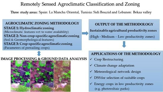
The objective of this paper is to identify and classify high-resolution sustainable agricultural productivity zones (high, medium, or low), in semi-arid and arid environments by considering a set of climatic, geomorphological, and vegetation data. In order to achieve the above objective, hydroclimatic classification is developed leading to water-limited growth environment (WLGE) zones based on aridity and drought indices. This is followed by further analyses of the soil and land-use features along with slopes, elevation, and similar topographic characteristics, leading to non-crop-specific agroclimatic zones; finally, crop-specific agroclimatic zones are produced, which identify sustainable productivity zones based on crop parameters. This paper is organized as follows: Section 2 presents background information and the existing knowledge of agroclimatic classification and zoning; Section 3 describes the methodological framework of agroclimatic classification and zoning, which includes the three stages to be followed, namely, hydroclimatic zoning, non-crop-specific agroclimatic zoning, and crop-specific agroclimatic zoning; Section 4 delineates the study areas and the database for each stage, along with pre-processing and processing approaches; and Section 5 presents the analysis and discussion of the results.

2. Background

The Food and Agriculture Organization (FAO) of the United Nations, in collaboration with IIASA (International Institute for Applied Systems Analysis), Laxenburg, Austria, has initiated the concept and developed the methodology of the agro-ecological zoning (AEZ) system, based on the principles of land evaluation. [1,2]. Moreover, in the AEZ system, socio-economic and institutional aspects, along with the availability and quality of water resources, constitute significant factors for food security. Individual crops are produced under specific soil, terrain, and agroclimatic conditions for a specific level of agricultural inputs and management conditions, which characterize the crop cultivation potential. In other words, the suitability of land for the cultivation of a given crop is based on crop requirements as compared to the prevailing agro-edaphic and agroclimatic conditions. The global AEZ (GAEZ) combines these two components by successively modifying grid-cell-specific agroclimatic suitability based on the edaphic suitability of location-specific soil and terrain characteristics.

In GAEZ, geo-referenced soil, terrain, and global climate data are combined into a land resource database, commonly assembled based on global grids. Precipitation, temperature, wind speed, sunshine hours, and relative humidity are the climatic data which are used to compile agronomically meaningful climate resource inventories, including quantified thermal and moisture regimes in space and time. At first, the crop-specific limitations of prevailing soil, terrain, and climate resources are identified and evaluated using simple and robust crop models, under assumed levels of inputs and management conditions. Then, matching procedures provide maximum-potential and agronomically attainable crop yields in the framework of basic land resource units, based on different agricultural production systems, which are defined by the levels of inputs and management conditions along with water supply systems. The resulting generic production systems are referred to as land utilization types (LUT). Indeed, for each LUT, the GAEZ procedures are applied either for rain-fed conditions or for conditions with specific water conservation practices, as well as for irrigated conditions. Nevertheless, calculations are conducted for different levels of inputs and management assumptions.

Moreover, conventional statistical methods are based on the ability to obtain observations from unknown true probability distributions. However, global change processes create new estimation problems since they require recovering information from only partially observable or even unobservable variables. Typical examples are the available agricultural production databases at the global and national level, respectively. There is thus an information gap between simulated potential yields and observed yields of crops currently grown. Indeed, GAEZ mainly develops large databases of natural resources focusing on crop suitability and attainable yields, which are related to agricultural uses and spatially detailed results of individual LUT assessments. These databases constitute the basis for the quantification of land productivity. Moreover, various applications are considered, such as major land use/cover patterns, land protection status, or classes reflecting infrastructure availability and market access conditions.

Agroclimatic classification methodologies have been developed based on FAO’s agro-ecological zoning (AEZ) approach to identify optimal and non-optimal agricultural productivity zones. It is recognized that yield is determined by weather conditions, whereas climate, which is among the most important factors, determines crop suitability and the agricultural potential in a region [27]. Indeed, studies addressing the impact of climate variability and change in viticulture are particularly pertinent, as climate is the leading factor for grapevine yield and quality [28,29] and for grapevine global geographical distribution [30]. The quantity and spatiotemporal variability of precipitation and temperature are variables which determine the type of crops suitable to a given location, and all agroclimatic classification methodologies utilize these variables [31]. Moreover, merging soil types and geomorphology with these climatic parameters can determine areas where high levels of production are appropriate, avoiding the threat of degrading natural resources. The required quantity of rainfall for crop production differs from region to region, mainly due to water balance conditions, i.e., the decreasing “effectiveness” of rainfall to maintain plant growth due to increasing evaporation [32]. Effective rainfall is related to the available moisture in the plant’s root zone, allowing the plant to germinate, emerge, and maintain its growth.

The agroclimatic characterization of crops includes temperature, humidity, solar radiation, and photoperiod among its most important climatological factors. Agro-ecological zoning (AEZ) systems use data and models for the construction of suitability maps for agriculture. Indeed, the agro-ecological zoning (AEZ) methodology developed by FAO is the main system for land resource assessment. The AEZ concept involves the representation of land in spatial layers and the combination of these layers using GIS techniques. AEZ uses various databases, models, and decision support tools. The selection of crop varieties based on agroclimatic requirements involves the comparison of the regional availability of agroclimatic resources and the climatic requirements of certain crop varieties based on which the selection is to be made. Nevertheless, the selection of plant varieties at the local or regional level should be based on agroclimatic analyses, which contribute to determine the climatic requirements of the different crop varieties. The AEZ methodology, along with supporting software packages (ArcGIS 10.8.1), can be applied at the global, regional, national, and sub-national level.

Nevertheless, the availability of sufficient water remains a requirement in crop production. During the growing season in irrigated and rainfed agriculture, water is often the limiting factor for production. Indeed, during the growing season, the temporal pattern of water availability for plant use and the ensuring crop biomass and yield are determined by the quantity and distribution of rain and supplemental irrigation, along with soil features and evapotranspiration losses [11]. There are many climatic and agroclimatic classifications, which delineate the moisture conditions of crops [33]. These classifications vary in complexity based on the number of parameters used. Most of these agroclimatic classification approaches use potential evapotranspiration and rainfall to delimit the growth environment of crops [21]. Indeed, in Burkina Faso, where rainfed production is a major source of food and income, an investigation has been conducted of the water-limited growth environment (WLGE) for millet cultivation. Specifically, in Badini’s study, the aridity index (AI) and crop water stress index (CWSI) have been used to define such environments [21]. The vegetation health index (VHI) has also been proposed for monitoring the impact of weather on vegetation and used it for monitoring production and agricultural drought [34].

In addition, multi-scaling agroclimatic classification at the meso-scale level has been applied for the development of viticultural zoning at the European scale, based on climate model simulations and bioclimatic indices [12]. It seems that winegrapes are likely to face new challenges in the coming decades due to climate change. Shifts in yield and ripening potential, grapevine phenology, disease and pest patterns, and wine styles are projected to take place in response to future conditions [35]. By considering the interactions between winegrape climatic requirements and its growing cycle, several climate-based (bioclimatic) indices have been proposed to describe the suitability of different winegrowing areas. The proposed combination of all these indices can achieve finer scale agroclimatic classification even in hilly terrain. As a result, optimal production can be computed for each sustainable production zone, at a multi-scale level.

It is worth mentioning the use of satellite data and methods. Indeed, the main driving force behind the use of satellite data for the computation of indices in agroclimatic zoning is the lack of long records from weather stations in many developing areas, as well as the lack of available data in remote areas [18]. Indeed, remote sensing technologies and products have gradually become an important tool for the detection and the spatiotemporal distribution and characteristics of environmental variables at different scales. Moreover, there is a gradually increasing reliability and accuracy in remote sensing data and methods [36]. In addition, new satellite systems carry more bands, have higher spatial resolution, and new sensors for environmental parameters and vegetation [37].

The growing technological advancements also offer additional computational capabilities. The trend is to extract data from gridded satellite datasets and biophysical data. This is particularly useful when dealing with the combined use of several satellite systems, where the selected cell resolution is that of the coarsest input dataset [38,39]. Moreover, analytical tools for working with big datasets make it possible to extract new information from environmental satellites with varying spatial resolution, such as Landsat-8 imagery (30 m), RapidEye (5 m), Worldview-3 (0.31 m), or Pleiades (0.5 m). Thus, digital data processing and analysis for agroecosystems, including satellite imagery, monitoring, and preparedness planning, including decision support systems (DSS), could be incorporated into a dynamic web production platform. Moreover, new satellite systems offer online open information for web platforms [17,40].

In this paper, the developed and applied agroclimatic classification methodology is essentially based on FAO’s agro-ecological zoning (AEZ) approach. Specifically, the applied methodology follows Badini’s approach [21] with the inclusion of satellite data and methods [11,17]. The developed methodology consists of three distinct stages (steps): the first stage, called hydroclimatic zoning, deals with the micro-climatic features of the selected region through the computation of drought indices, where the outcome of hydroclimatic zoning is the water-limited growth environment (WLGE) zones. Stage two consists of the so-called non-crop-specific agroclimatic zoning, which is superimposed to the stage one outcome, and where soil types and features, land use/land cover features, and landforms (digital elevation models (DEM), slopes) are considered for assessing the land’s suitability for agricultural use. Finally, stage three, called crop-specific agroclimatic zoning, deals with the prevailing crop characteristics through the computation of parameters, leading to agricultural productivity (high, medium, or low) zones. This methodology was initially applied in Thessaly Greece more than ten years ago [11], using satellite data of the previous generation, such as NOAA, with a resolution of 8 × 8 km, whereas the current application uses Landsat-8 with a resolution of 30 × 30 m, which leads to an extremely detailed spatial analysis and classification.

3. Materials and Methods

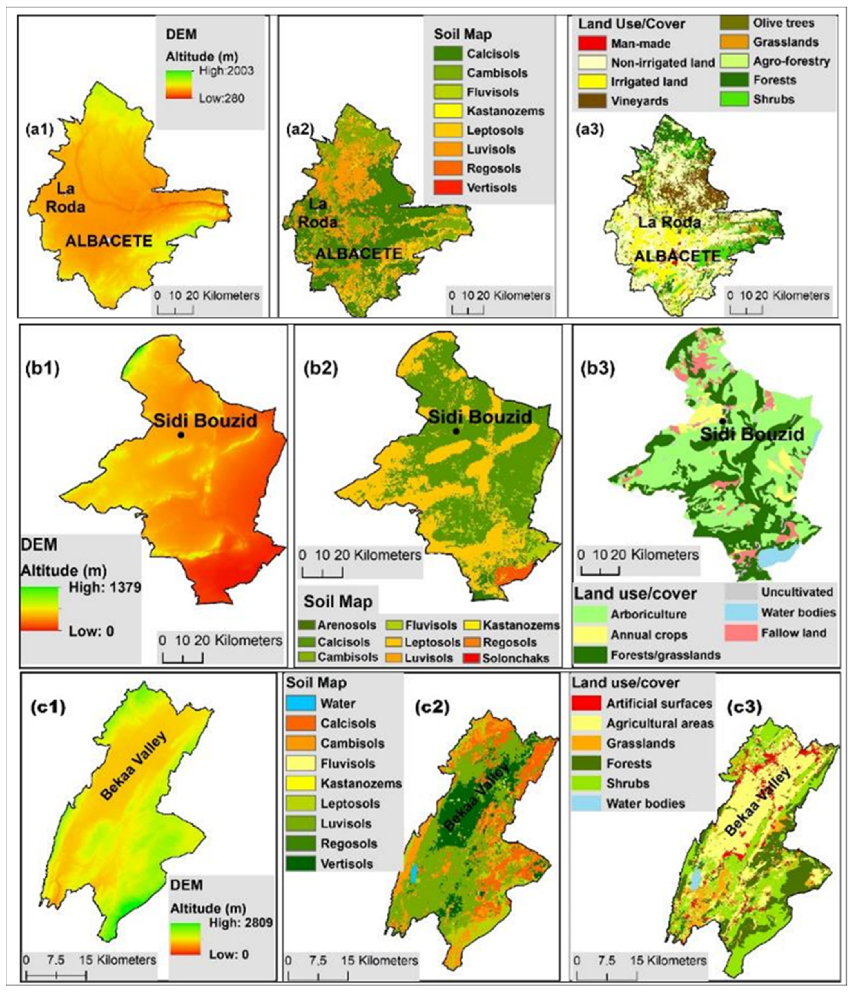
This study evaluates the new Earth observation datasets and methodological approaches provided by the Google Earth Engine (GEE) platform. The proposed and developed methodology is implemented in three study areas in the Mediterranean basin, namely, in the “La Mancha Oriental” region in Spain, “Sidi Bouzid” region in Tunisia, and “Beqaa” valley in Lebanon.

➢

Methodological steps

The proposed methodology is based on GIS and remote sensing techniques for considering climate, soil, and topography restrictions in creating sustainable crop production zones. Shortly, the three basic steps that characterize this methodology are as follows [11,24]: (a) Hydroclimatic zoning. The water availability is studied, based on drought indices (aridity index (AI) and vegetation health index (VHI)), and leading to water-limited growth environment (WLGE) zones. (b) Non-crop-specific agroclimatic zoning. Apart from water shortage, soil, land- use/land cover features, and landforms (digital elevation models (DEM), slopes) are considered for assessing the agricultural land suitability in general. (c) Crop-specific agroclimatic zoning. For specific crops (or families of crops), components as growing degree days (GDD), net radiation (Rn), and spring precipitation are calculated as indicators for assessing crop development restrictions.

These three basic steps are illustrated in the following flow-chart (Figure 1).

➢

GEE platform and downscaling machine learning approaches

Google Earth Engine (GEE) is used for processing geospatial datasets spanning over 20 years of EO imagery. Moreover, downscaling methods are applied for acquiring fine resolution data from datasets having a coarse spatial resolution. The main idea of this method is to establish the correlation between coarse resolution variables and finer environmental variables (normalized difference vegetation index, NDVI, digital elevation model, etc.), and then use finer environmental indicators as input to downscale remote sensing data from a coarse resolution to a fine resolution [41]. Especially for the precipitation data, machine learning approaches have been proved considerably effective in the downscaling approach based on land surface characteristics [42,43,44]. Thus, the machine learning algorithm classification and regression tree (CART) is implemented for acquired data at a higher resolution pixel size. The three methodological steps of agroclimatic classification are thoroughly described in the following sections.

3.1. Hydroclimatic Zoning

The first step in agroclimatic classification procedure is the calculation of water-limited growth environment (WLGE) zones. The two indices, vegetation index (VHI) and aridity index (AI), are combined in order to create the WLGE zones which describe the hydroclimatic conditions of the study area [45,46]. VHI is an index of agricultural drought and represents overall vegetation health (moisture and thermal conditions); it is suitable for the identification of vegetation stress, especially in cases where no specific crop is examined. AI is used to determine the adequacy of rainfall in satisfying the water needs of crops. The two indices are used to define zones suitable for agricultural use according to water limitations.

3.1.1. Vegetation Health Index (VHI)

The VHI is a one of the most famous satellite-based indices for drought analysis. It is used especially for the identification of agricultural drought assessment, according to climate conditions (moisture and thermal conditions) [22]. The vegetation stress is implied by a low NDVI and a high land surface temperature (LST) [47]. The VHI is calculated using two components: the vegetation condition index (VCI) and the thermal condition index (TCI) [48].

The VCI, which is derived from long-term satellite data (i.e., Landsat, etc.), is based on the NDVI. The NDVI is a measure of vigor or vegetation stress. NDVI is (NIR-R)/(NIR + R) where NIR and R are the near-infrared and red reflectance, respectively. Negative NDVI values indicate clouds and water, positive values near zero indicate bare soil, sparse vegetation (0.1–0.5), and dense green vegetation (0.6 and above). During vegetation stress events, low NDVI values are expected. The VCI is computed applying the following equation [49]:

$$\mathrm{V}\mathrm{C}\mathrm{I}=\frac{{\mathrm{N}\mathrm{D}\mathrm{V}\mathrm{I}}_{\mathrm{i}}-{\mathrm{N}\mathrm{D}\mathrm{V}\mathrm{I}}_{\mathrm{m}\mathrm{i}\mathrm{n}}}{{\mathrm{N}\mathrm{D}\mathrm{V}\mathrm{I}}_{\mathrm{m}\mathrm{a}\mathrm{x}}-{\mathrm{N}\mathrm{D}\mathrm{V}\mathrm{I}}_{\mathrm{m}\mathrm{i}\mathrm{n}}}\ast 100$$

(1)

where NDVI_i is the value for each pixel at a given date, and NDVI_max and NDVI_min are the maximum and minimum values of NDVI for the considered pixel over the whole study period, respectively.

The TCI is based on information on the thermal infrared (TIR) part of the electromagnetic spectrum. The TCI monitors the stress of vegetation due to temperature. There is a direct impact to vegetation health by thermal conditions, especially when moisture scarcity is combined with high temperature. The TCI is defined by the equation [50]:

$$\mathrm{T}\mathrm{C}\mathrm{I}=\frac{{\mathrm{L}\mathrm{S}\mathrm{T}}_{\mathrm{m}\mathrm{a}\mathrm{x}}-{\mathrm{L}\mathrm{S}\mathrm{T}}_{\mathrm{i}}}{{\mathrm{L}\mathrm{S}\mathrm{T}}_{\mathrm{m}\mathrm{a}\mathrm{x}}-{\mathrm{L}\mathrm{S}\mathrm{T}}_{\mathrm{m}\mathrm{i}\mathrm{n}}}\ast 100$$

(2)

where LST_i is the land surface temperature (LST) for each pixel and a given date; LST_max and LST_min are the maximum and minimum values of LST for the considered pixel over the climatological period of study, respectively.

The values of the VCI and TCI components range from 0 to 100. Consequently, lower values indicate extremely unfavorable conditions and higher values represent healthy vegetation. The maximum/minimum values of both indices are based on the concept that a max/min amount of vegetation exists under optimal or unfavorable weather conditions, respectively.

The VHI is calculated using the following equation:

$$\mathrm{V}\mathrm{H}\mathrm{I}=\mathrm{a}\mathrm{V}\mathrm{C}\mathrm{I}+(1-\mathrm{a})\mathrm{T}\mathrm{C}\mathrm{I}$$

(3)

where a is the contribution of VCI and TCI to the VHI according to the environmental conditions. Since the contribution of water demand and temperature during the vegetation cycle is same, the coefficient a is assigned the value of 0.5 [47].

Finally, the values of the VHI equation range from 0 to 100, and are classified into five classes of agricultural drought as shown in the following table [34,51] (

Table 1. Classification of VHI values.

Drought Classes	Values
Extreme	0–10
Severe	10–20
Moderate	20–30
Mild	30–40
No drought	>40

).

3.1.2. Aridity Index (AI)

AI is the second index applied for creating WLGE zones. The Aridity Index (AI) is considered a permanent feature of the climate of the region and determines the efficiency of the water needs of rainfed crops [52]. The AI is calculated using meteorological data as a ratio of precipitation to potential evapotranspiration. Thus, the AI equation is [53]:

$$\mathrm{A}\mathrm{I}=\frac{{\mathrm{P}}_{\mathrm{i}}}{{\mathrm{P}\mathrm{E}\mathrm{T}}_{\mathrm{i}}}$$

(4)

where Pi is the monthly precipitation and PETi the monthly potential evapotranspiration.

The AI classifies arid regions into seven classes ranging from hyper-arid to very humid. The classification scheme is based on FAO [54] (

Table 2. Dryland categories of AI.

AI Aridity Classes	Aridity Index
Very Humid	AI ≥ 1.5
Humid	0.8 ≤ AI < 1.5
Sub-Humid	0.65 ≤ AI < 0.8
Dry Sub-Humid	0.5 ≤ AI < 0.65
Semi-Arid	0.2 ≤ AI < 0.5
Arid	0.05 ≤ AI < 0.2
Hyper-Arid	AI < 0.05

).

3.1.3. WLGE Zones

Since both indices (VHI and AI) have been calculated, the water-limited growth environment (WLGE) zones are created. The VHI map, which indicates the occurrence of agricultural drought, is combined with the climatic aridity map leading to the delimitation of the area in five hydroclimatic (WLGE) zones, as illustrated in the following table (

Table 3. WLGE classes.

Agricultural Drought Classes (VHI)	Aridity Classes (AI)	WLGE Zones
Extreme drought	Hyper-Arid	Limited environment
Severe drought	Arid	Limited/Partially limited environment
Moderate drought	Semi-Arid/Dry Sub-Humid	Partially limited environment
Mild drought	Sub-Humid	Partially limited/No limitations environment
No drought	Humid/Very Humid	No limitations

): No limitations, Partially limited/No limitations environment, Partially limited environment, Limited/Partially limited environment and Limited environment.

3.2. Non-Crop-Specific Agroclimatic Zoning

3.2.1. Multi-Criteria Decision Making

The second step is based on the creation of general agroclimatic zoning or non-crop-specific agroclimatic zones regarding water conservation, land fertility, and landform restrictions. Therefore, a GIS multi-criteria decision making (MCDM) method is applied by combining a set of criteria (variables), namely, WLGE zones, digital elevation model (DEM), slope, soil map, and land use/land cover [11]. The GIS-MCDM model appraises each criterion according to its importance concerning the optimal crop growth conditions [55]. Subsequently, each criterion is classified in a range from 10, which indicates a more suitable agricultural zone, to 0.

The exact ratings of the suitability of land for agriculture for each criterion depends on the special characteristics of each study area. An expert opinion analysis additionally to the relevant bibliography must be conducted to achieve high fidelity and reliable results. For instance, the slope ranking classes are obtained based to the Storie soil-based classification system [56,57]. An indicative example of the above-mentioned classification is presented in the following table (

Table 4. Ratings and suitability classes assigned to each criterion for agricultural suitability.

Criteria	Classes	Ratings	Agricultural Land Suitability
Digital elevation model (DEM)	0–400	10	Good
	400–600	9	Fair
	600–800	8	Moderate
	800–900	7	Average
	900–1000	5	Poor
	>1000	0	Not suitable
Slope %	0–2 (Nearly Level)	10	Good
	2–8 (Gently Sloping)	9	Fair
	8–15 (Moderately Sloping)	8	Moderate
	15–30 (Strongly Sloping)	6	Average
	30–45 (Steep)	2	Poor
	>45 (Very Steep)	0	Not suitable
Soil map	Fluvisols (Agricultural Use)	10	Good
	Cambisols (Agricultural Use)	9	Fair
	Luvisols (Agricultural Use)	9	Fair
	Calcisols (Controlled Agricultural Use)	5	Average
	Regosols (Controlled Agricultural Use)	5	Average
	Kastanozems (Controlled Agricultural Use)	2	Poor
	Leptosols (No Agricultural Use)	1	Poor
Land use/land cover	Annual crops	10	Good
	Arboriculture	9	Fair
	Grasslands	4	Poor
	Man-made areas/Water bodies/Forests, etc.	0	Not suitable
WLGE zoning	No Limitations	10	Good
	Partially limited/No limitations	9	Fair
	Partially limited	8	Moderate
	Limited/Partially limited	6	Average
	Limited environment	2	Poor

), which may be different from region to region.

Furthermore, the derived weight of each criterion is estimated via the analytical hierarchy process (AHP), through pairwise comparison. This is one of the most widely accepted methods in the MCDM process [58].The AHP method is developed in three steps [59]:

-

Step1: Identification of the set of suitable criteria

-

Step2: The relative importance between pairs of criteria.

-

Step3: The consistency of the pairwise comparisons

The degree of consistency in assigning weight among criteria is tested using the consistency ratio tool. A reasonable level of pairwise judgment is accepted with a consistency ratio of 0.10 or less [60,61].

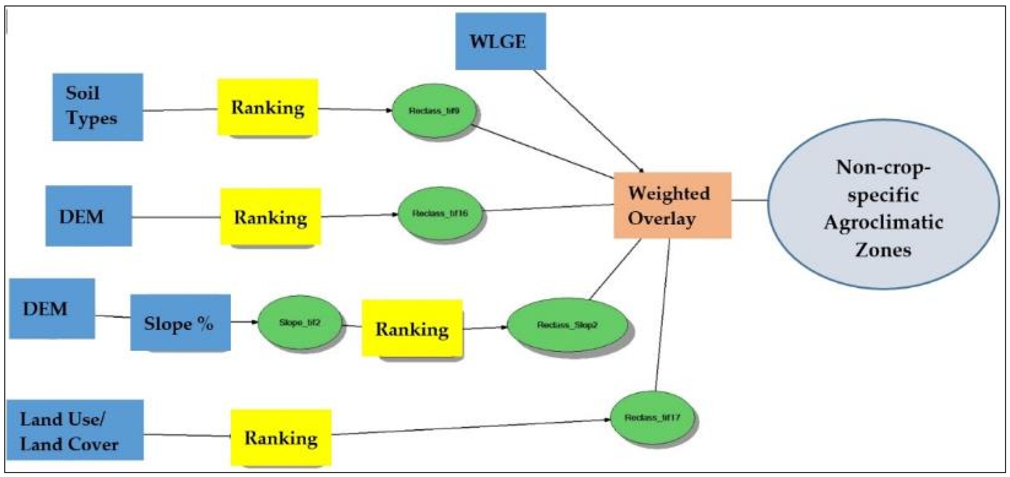
3.2.2. Non-Crop-Specific Model

A GIS multi-criteria model combining the spatial variables is created (Figure 2). Firstly, a geospatial database is created using a GIS software (ArcGIS 10.8.1) for data analysis. Then, the thematic maps are transformed into a raster format. Then, the ranking of the variables (WLGE, soil types, DEM, slopes, and land use/land cover) is considered. Next, the weights for each variable, as derived from the AHP, are imported in the model. Subsequently, the layers are combined. Finally, the derived thematic map leads to five non-crop-specific agroclimatic suitable classes: Good, Fair, Moderate, Poor, and Not Suitable.

3.3. Crop-Specific Agroclimatic Zoning

The suitable zones for each crop or group of crops (e.g., winter/summer crops) is represented in crop-specific agroclimatic zoning. To create these classes, three basic parameters are considered in order to identify areas suitable for each crop, namely, growing degree days (GDD), net radiation (Rn), and the amount of spring precipitation.

3.3.1. Growing Degree Days °C

Temperature is one of the main factors for plant growth. The growing degree days (GDD) are a weather-based indicator and are used to predict crop development. They determines the accumulated heat units for a crop during the growing season. The GDD are calculated as the air temperature daily average accumulation above a minimum threshold temperature during the crop lifetime. The basic concept is that crop growth will occur if the temperature exceeds the base threshold temperature [62,63,64]. The following equation is used for the season GDD (°C d) estimation [65].

$$\mathrm{G}\mathrm{D}\mathrm{D}=\sum _1^{\mathrm{n}}{\mathsf{\delta }}_{\mathrm{i}}\ast ({\mathrm{T}}_{\mathrm{m}\mathrm{e}\mathrm{a}\mathrm{n}}-{\mathrm{T}}_{\mathrm{b}\mathrm{a}\mathrm{s}\mathrm{e}})$$

(5)

where n = growing season, T_mean > T_base then δi = 1, when T_mean < T_base then δi = 0. T_mean is the average daily temperatures during the crop growing season. T_base is the base threshold temperature for each crop.

The GDD estimations are performed over the basic crops in the study area. For each crop the base temperature and the optimum cumulative daily temperature for the growing season are determined. The GDD are the degree-day sum over the growing season (e.g., April–October) per pixel per year; then, the final product is the median value of the annual GDD over 20 years (2001–2020).

3.3.2. Net Radiation (Rn)

Solar radiation is the energy source for crop growth. Net radiation flux (Rn) represents the actual radiant energy available at the Earth’s surface [66]. Rn is used to delineate areas where crop growth is not restricted due to radiation. Rn is defined as the difference between incoming and outgoing longwave and shortwave radiation. Consequently, for the estimation of Rn, incoming and outgoing radiant fluxes are calculated, based on the surface radiation balance equation [67,68]:

Rn = (1 − α)R_S↓ + R_L↓ − R_L↑ − (1 − ε_o)R_L

(6)

where:

R_S↓ is the incoming shortwave radiation (W/m²),

α is the land surface reflectance albedo (dimensionless),

R_L↓ is the incoming longwave radiation (W/m²),

R_L↑ is the outgoing longwave radiation (W/m²), and

ε_o is the broad band surface emissivity (dimensionless).

The net radiation balance is represented in the following figure (Figure 3). From the initial downward shortwave radiation (R_S↓) value (gain), a portion of a R_S↓ is a loss. The R_S↓ is estimated by using the solar constant, the atmospheric clear sky shortwave transmission factor, the solar zenith angle, and the relative Earth–Sun distance. Moreover, the reflection coefficient, albedo α, is the proportion of the radiation that is reflected from a surface. It can be calculated from satellite data for each spectral band separately [69]. Similarly, from the initial downward longwave radiation R_L↓ (gain), a portion of (1 − ε_o) R_L↓ is a loss. The R_L↓ can be expressed using the Steffan–Boltzmann equation with atmospheric transmissivity and land surface temperature. Finally, R_L↑ is the outgoing longwave radiation emitted from the vegetation surface under consideration. It is estimated using the Stefan–Boltzmann equation with a calculated surface emissivity and surface temperature. All these variables can be computed using satellite data for a median long period [70,71,72,73].

3.3.3. Spring Precipitation

Another limiting factor for plant growth, the amount of precipitation in spring and mainly the last and the first 10 days of April and May (20 days in total), is also considered. Consequently, areas with a sufficient amount and timing of rainfall during this period are considered as the most suitable for annual crops, especially for winter cultivations. In order to calculate the median cumulative amount of precipitation, for the twenty days in spring, long time period earth observation data are implemented.

3.3.4. Crop-Specific Agroclimatic Map

Firstly, the GDD and Rn indicators are classified into three zones, namely, high, medium, and low productivity, in accordance to the type of crops, i.e., winter, summer, annual cultivations, etc. Secondly, the 20 days’ amount of spring rainfall (April–May) map is classified as sufficient or insufficient rain for annual crops. Finally, a combination of the previous variables identifies three classification zones: high, medium, and low productivity.

Subsequently, the three classification zones are combined with the non-crop-specific agroclimatic zoning. The final product is a crop-specific agroclimatic map divided in seven classes which are ranging from the most suitable to the not suitable zones for crop production. Particularly, the areas are classified as follows: (a) “Excellent”, “Very Good”, and “Good” are areas generally suitable for annual crops; (b) “Fair”, “Moderate”, and “Poor” are areas generally suitable for trees crops, vineyards, or annual crops under restrictions; and (c) “Not Suitable” are areas unsuitable for agricultural use.

4. Study Areas and Database

To evaluate the proposed methodology, three study areas around the Mediterranean Sea are considered. These areas are characterized by a semi-arid to arid climate with an intensive agricultural production system.

4.1. Description of Study Areas

• Spanish study area

The Spain pilot area is the region of “La Mancha Oriental”, located in the southeast of the Iberian Peninsula (Figure 4). The total land area is about 7100 km² (710,347 hectares), characterizing by a relatively level surface of land averaging from 500 m to 2000 m altitude. The climate can be classified as semi-arid with reference evapotranspiration above 1200 mm. The mean temperature varies between 5 °C in January and 24 °C in July, and the annual precipitation, in dry and wet years, fluctuates from 124 mm to 750 mm. The population is about 400,000 people, with the biggest town, Albacete, having 170,000 inhabitants.

The soil is highly variable with loam, sandy loam, and clay loam texture, often stony but easy to cultivate, and quite fertile under appropriate agronomic management. The region has a strong agriculture economy. About 500,000 ha are characterized as cultivated land with dominant annual crops (wheat, barley, alfalfa, onion, garlic, and legumes), fruit trees (almond, olive, and pistachio) and vineyards.

B.

Tunisian study area

The Tunisian pilot area is the province “Sidi Bouzid” (Sidi Bouzid Governorate), located in the central-western part of the country, in the semiarid land south of the Dorsal Mountains (Figure 5). The region occupies about 7472 km² (747,280 hectares), with a relatively flat surface and an average height of 300 m. The climate is semi-arid to arid in the south, with annual precipitation ranging from 300 to 200 mm. Almost 33,000 farms occupy about 380,000 ha of cultivated land. Soils are deep with an organic matter content ranging from 0.5 to 1.5%, being suitable for most of the crops. The most common crops in the area are fruit trees (olive, almond, and pistachios), vegetables crops (onion, pepper, tomatoes, and potatoes) and cereals, mainly durum wheat and oats.

C.

Lebanon study area

The Lebanon pilot area is the governorate of Bekaa, located in the central-eastern part of the country (Figure 6). The governorate has an area size about 1405 km² (140,463 hectares), with an altitude fluctuating between 800 m and 1000 m. The population is about 520,000 residents. The soils are formed mainly of limestone, dolomite, and sedimentary carbonate rocks, and are characterized by a high clay content (50%) and relatively low organic matter. At the Bekaa valley, the main type of soil is Eutric Cambisols changing to Lithic Leptosols on both sides of the valley. The Bekaa valley is the main agricultural land located between the two mountain chains of Lebanon, Mount-Lebanon and Anti-Lebanon. The irrigated part of this land is 69%, which represents 42% of the national agriculture production.. In proportion, one-third of the main crops are wheat and other winter cereals, mainly barley, one-third are potato, winter legumes, and summer vegetables (watermelon, cucumbers, and bell pepper), and one third are fruit trees (apples and peaches), olives, vineyards, and land kept as fallow during the in-between seasons.

4.2. Dataset and Preprocessing

4.2.1. Hydroclimatic Zoning Database

To identify WLGE, the first index, VHI, is calculated from Landsat-8 multispectral satellite data, with a 30-m spatial resolution. The available derived Landsat data are for the period from 2013 to 2020. For the study areas in Spain, Lebanon, and Tunisia, 642, 329, and 823 Landsat images are processed, respectively, in the GEE platform. Subsequently, the second WLGE index, namely, AI, is calculated using Earth observation (EO) data for a period of twenty years (2001–2020). Specifically, the multi-year analysis is implemented in the GEE platform using the following EO data:

• The Climate Hazards Group InfraRed Precipitation with Station data (CHIRPS). This is rainfall product of more than 36 years integrating satellite information and in situ station data. The spatial resolution is 0.05° (5 km approximately) [74]. The preprocessing of pentad CHIRPS data is applied (2001–2020) to achieve temporal compatibility with other EO data, such as MODIS data. Specifically, the mean monthly rainfall is calculated first and then the median monthly rainfall for each pixel is estimated for the time period under consideration (2001–2020). For each area of research in Spain, Lebanon, and Tunisia, 1440 pentad data are processed (4320 images in total).
• The MODIS 8-day Evapotranspiration/Latent Heat Flux product (MOD16A2). It is an 8-day composite dataset providing, among other, the potential evapotranspiration layer (PET) at a 500 m spatial resolution. The analysis of PET products is conducted from https://doi.org/10.5067/MODIS/MOD16A2.006, [accessed date on 1 April 2023] between 2001 and 2020. Specifically the mean monthly PET is calculated first and then the median monthly PET, is estimated for each pixel. In each study area, in Spain, Lebanon, and Tunisia, 919 8-day datasets are processed (2757 images in total).

4.2.2. Non-Crop-Specific Agroclimatic Zoning Database

To create non-crop-specific agroclimatic zoning, a variety of geospatial data, in different spatial and temporal resolutions, are downloaded. In general, the following datasets are prepared:

• Digital elevation model (DEM) [75]. The DEM dataset is derived from the Shuttle Radar Topography Mission (SRTM) project provided by NASA. The DEM has a spatial resolution of about 30 m.
• Soil maps. The Soil dataset of the three study areas is derived by the International Soil Reference and Information Centre (ISRIC) at 250 m resolution [76]. The soil classification based on an international system for classification of soils named World Reference Base (WRB).
• Land use/land cover (LU/LC). For the Spanish study area, the Corine Land Cover (CLC) product (2018), is used, as obtained from the Copernicus Land Monitoring Service [77]. The CLC product has a 25-hectare minimum mapping unit for areal phenomena and a 100 m minimum width for linear phenomena. For the study areas in Tunisia and Lebanon, relevant thematic maps are provided by the local institutions.

4.2.3. Crop-Specific Agroclimatic Zoning Database

Also, the three variables for the calculation of crop-specific agroclimatic zoning, namely, growing degree days (GDD), net radiation (Rn), and precipitation, are estimated using EO data in GEE:

• The GDD is calculated based on two datasets: (a) Initially the ERA-5 reanalysis dataset is processed for a time-period of 31 years (1990–2020). This dataset provides aggregated daily values for several climatic reanalysis parameters (2 m air temperature, total precipitation, etc.) [78]. The ERA-5 was not used, since the main disadvantage of these data is the low spatial resolution (pixel size 30 km approximately). (b) The second approach is based on the MODIS (MOD11A2 V6) product [79]. This is an average 8-day land surface temperature dataset at 1 km spatial resolution. The final GDD is calculated by estimating the median value of the annual GDD over 20 years (2001–2020). The second approach is adopted for the calculation of the GDD in the three study areas because of the higher spatial resolution. For instance, for winter crops, in each research area, 420 8-day MOD11A2 datasets are processed (1260 images in total).
• The net radiation is calculated based on Landsat-8 satellite data for the period 2013–2020. This dataset contains atmospherically corrected land surface temperatures. For each study area, in Spain, Tunisia, and Lebanon, 642, 823, and 329 Landsat images are processed, respectively.
• Finally, the 20-day spring cumulative precipitation is estimated using 36-year CHIRPS pentad precipitation data (period 1984–2020). For each study area, 168 datasets are analyzed and then the median cumulative precipitation for each pixel (for the 20-day period) is estimated.

4.3. Applied Methodology

The three steps of the proposed methodology for agroclimatic zoning are applied in the three study areas, La Mancha Oriental, Sidi Bouzid, and Bekaa governorate, as described below.

4.3.1. Hydroclimatic Zones

I.

Vegetation Health Index (VHI)

Firstly, the vegetation health (VHI) is derived in the three study areas. In the figure below, the median VHI for the 8-year period is presented (Figure 7). Two classes, “No Drought” and “Mild Drought”, prevail in the three study areas.

II.

Aridity Index (AI)

Secondly, the median AI is calculated for the 20-year period. Also, a downscaling resampling method is applied to achieve a 30-m spatial resolution. In the following figure, the aridity index (AI) classes for the three study areas are illustrated (Figure 8). In the “La Mancha Oriental” region, the semi-arid class prevails, while in the “Sidi Bouzid” and “Bekaa” governorates, the arid class occupies most of their areas.

III.

Water-Limited Growth Environment (WLGE) Zones

Finally, a thematic map, containing the water-limited growth environment (WLGE) zones, is created. As is illustrated in the following figure, the dominant classes for the “Sidi Bouzid” and “Bekaa” governorates are the “limited” zones, while for the “La Mancha Oriental” region, they are the “partially limited” zones (Figure 9).

4.3.2. Non-Crop-Specific Agroclimatic Zoning

The DEM, soil, and land use/land cover maps are downloaded and processed for the three study areas (Figure 10). Indeed, the slope is produced from the DEM, it is incorporated into the procedure, and the DEM is presented (Figure 10). To achieved effective conclusions about the agricultural suitability of the land, the following spatial variables are considered: WLGE zone, soil map, DEM, slopes, and land use/land cover. Their behavior with respect to sensitivity among the other classes is tested, and finally a ranking, from 10 (suitable) to 1 (not suitable), according to agricultural suitability is applied. Higher ranking data indicate a better influence of agriculture. Finally, through the multi-criteria analysis, the non-crop-specific agroclimatic zoning maps are created in the three research areas.

4.3.3. Crop-Specific Agroclimatic Zoning

For the three study areas, winter annual crops are considered for identifying suitability zones. Specifically, the crop types are illustrated in the following table (

Table 5. Winter crops in the study areas.

	Crop Type
Spain	Barley, garlic, oat, wheat
Tunisia	Oat, wheat
Lebanon	Wheat

).

Consequently, the variables growing degree days (GDD), net radiation (Rn), and cumulative precipitation in April–May, are estimated based on the abovementioned winter crops in each one of the three areas.

I.

GDD: Growing Degree Days °C

Firstly, the range of optimum GDD and the base temperature for the crops during the growing season in the three study areas are presented, as provided by local authorities [80,81,82] (

Table 6. The range of optimum GDD for the growing of crops [80,81,82].

Study Area	Crop Type	Tbase	Tsum °C-d	Growing Season
Spain	Barley	2	1250–1600	December–June
	Garlic	0	1900–2004	December–June
	Oat	2	1480–1740	December–June
	Wheat	2	1540–1660	December–June
Tunisia	Oat	2	1891	December–June
	Wheat	2	1646	December–June
Lebanon	Wheat	6	1800–2000	December–June

).

Next, the calculation of GDD using the ERA-5 reanalysis dataset is performed. For instance, the averaging of 31 years (1990–2020) GDD for wheat in the study area “La Mancha Oriental” (Spain) is illustrated below (Figure 11).

Finaly, the GDD maps are calculated based on 8-day LST using the MODIS product at 1 km spatial resolution because the ERA5 reanalysis data (30 km) have a low spatial resolution. After the applied downscaling technique on the MODIS data, 30-m pixel size maps are created for the three study areas (Figure 12).

II.

Net Radiation

Accordingly, net radiation is considered. The median Rn map of each one of the three study areas is calculated with a spatial resolution of 30 m (Figure 13).

III.

Amount of Spring Precipitation

The median cumulative amount of 20 days’ precipitation (April to May) is estimated using the 37-year CHIRPS data (Figure 14).

The threshold of 20 mm of precipitation (for the range of 20 days) is used for the Spain study area and 10 mm for the Tunisia and Lebanon study areas, respectively. This differentiation was considered due to the different prevailing climate conditions in the regions “Sidi Bouzid” and “Bekaa” valley, as compared to the “La Mancha Oriental” region in Spain. These thresholds are applied in the first two best suitable classes of non-crop-specific agroclimatic zoning. The reason is that these two classes may be suitable for sustainable annual crops production by rainfed water supply.

5. Results

5.1. Non-Crop-Specific Agroclimatic Map

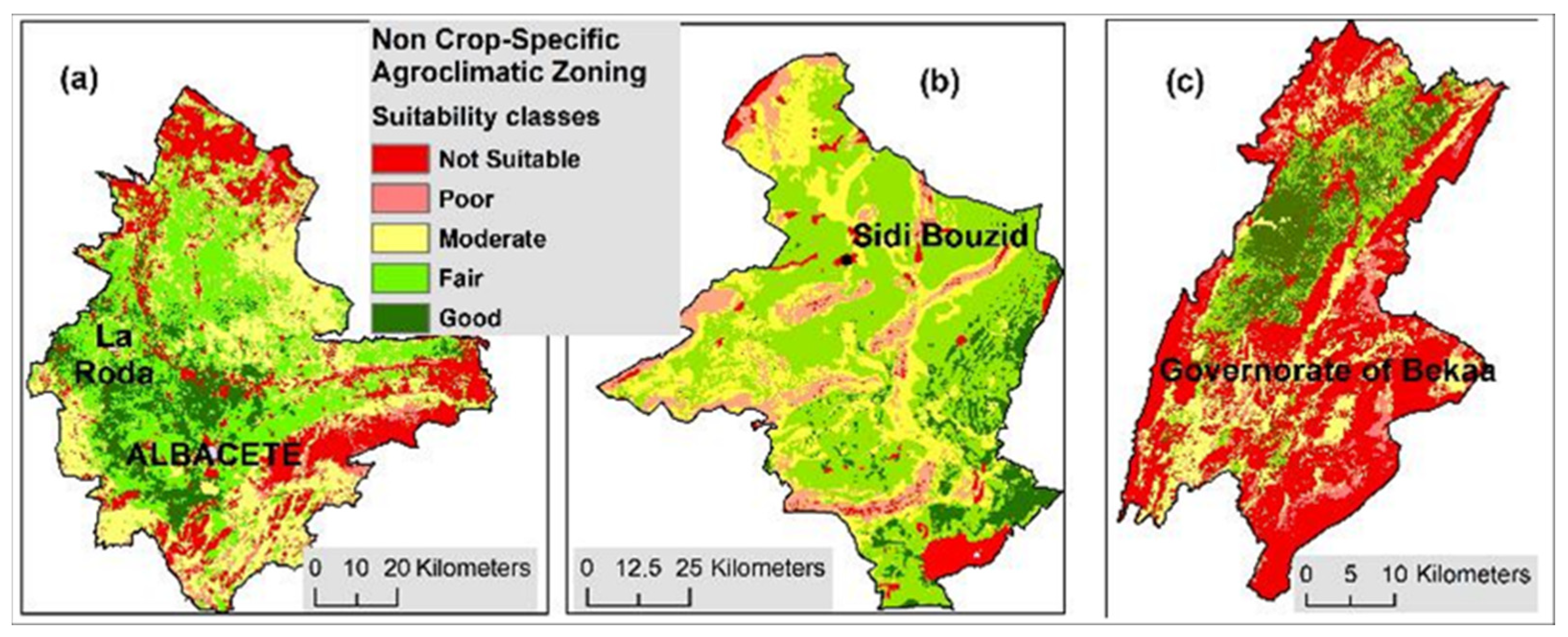
The non-crop-specific agroclimatic map for each one of the study areas is divided into five land suitability zones for agricultural purposes, i.e., Good, Fair, Moderate, Poor, and Not Suitable (Figure 15).

Next, acreage and the percentage of each zone are calculated using statistical analysis (

Table 7. Area covered by each non-crop-specific zone in the three study areas.

Non-Crop-Specific Agroclimatic Zones	La Mancha Oriental (Spain)		Sidi Bouzid (Tunisia)		Governorate of Bekaa (Lebanon)
	Acreage (Ha)	%	Acreage (Ha)	%	Acreage (Ha)	%
Good	76,345	10.7	58,420	7.8	17,935	12.8
Fair	240,022	33.8	365,582	48.9	15,221	10.8
Moderate	208,241	29.3	194,855	26.1	25,267	18
Poor	31,699	4.5	86,230	11.5	10,183	7.2
Not Suitable	154,040	21.7	42,193	5.7	71,857	51.2
Sum	710,347	100	747,280	100	140,463	100

). Moreover, complementary research with local authorities has been helpful in better characterizing the suitability zones.

In the region of “La Mancha Oriental”, the best two suitability zones (good and fair), which are good enough for rainfed irrigation, cover approximately half of the total area (44.5%). In these zones, there are annual crops such as barley, wheat, alfalfa, onion, garlic, and legumes and woody crops (i.e., olives and pistachios). In the third class (moderate zones), vineyard cultivation is dominant, especially in the northeastern regions.

In the governorate of “Sidi Bouzid”, the best two suitability zones (good and fair) cover more than half of the total area (56.7%). In these zones, there are annual crops such as cereals and vegetables, and arboriculture, i.e., almond, pistachio, and olive trees. In the third class (moderate zones, 26.1%), livestock farming products are dominant.

In the governorate of “Bekaa”, the best two suitability zones (good and fair) cover 23.6% of the total area. These zones cover almost all the fertile Bekaa valley. In these zones, the main annual crops are wheat, barley, potato, and vegetables. Moreover, there is arboriculture, i.e., apples, peaches, olives, and vineyards.

5.2. Crop-Specific Agroclimatic Zoning Map

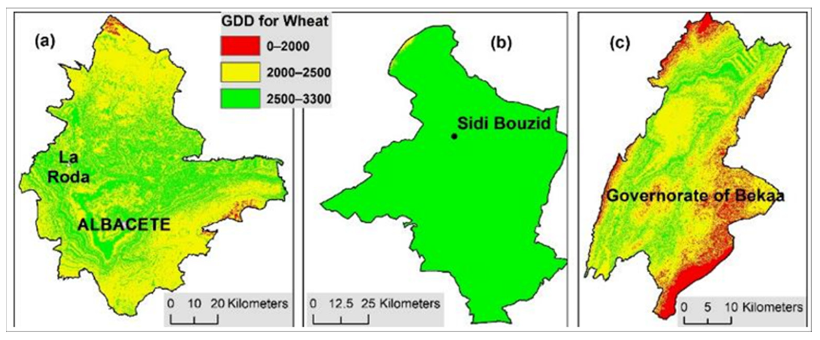
The analysis of the GDD and Rn shows that they are not limited factors for the annual winter crops and especially for wheat. In the “La Mancha Oriental” region, the GDD min, max, and mean values are 1799, 2875, and 2442, respectively. Most of the study area assigns values of GDD of more than 1500. Moreover, the Rn min, max, and mean values are 14, 980, and 710 (watt/m2), respectively. For the “Sidi Bouzid” governorate, the GDD min, max, and mean values are 2187, 3284, and 2985 °C, respectively. The lower values are in the northern part of the region. In addition, the Rn min, max, and mean values are 184, 992, and 599 (W/m²). For the “Bekaa” governorate, the GDD min, max, and mean values are 1123, 2888, and 2247 °C, respectively. The values below 1800 GDD are located in the southeastern and northern parts of the governorate, thus, outside the Bekaa valley. Furthermore, the Rn min, max, and mean values are 222, 894, and 679 W/m², respectively.

In contrast, the 20-day spring cumulative precipitation of April and May is a limited factor for the wheat winter crop. For the “La Mancha Oriental” region, the min, max, and mean precipitation values are 12.3, 31.7, and 20.5 mm, respectively. Most of the study area assigns precipitation values (for the 20 days in spring) in a range of 15–25 mm. 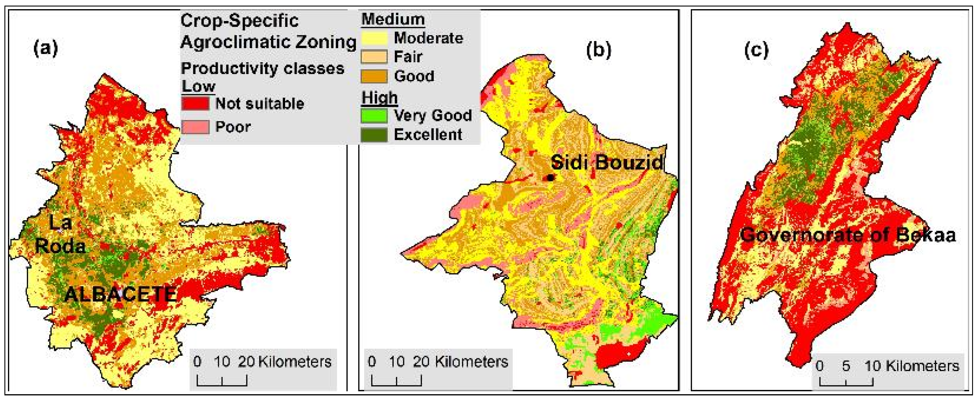Next, the “Sidi Bouzid” governorate has min, max, and mean values of 4.5, 23.1, and 11.5 mm, respectively (Figure 14). The precipitation of most cultivated areas has values less than 10 mm. Finally, the “Bekaa” governorate assigns 5.8, 19.6, and 12.8 mm as the min, max, and mean values, respectively. Especially for the Bekaa valley, the precipitation fluctuates between 10 and 15 mm. The result is a seven-class map in terms of sustainable wheat crop production (Figure 16).

The acreage and percentage of each one of the seven zones are calculated (

Table 8. The acreage and percentage of suitability zones for wheat crop sustainable production in the three study areas.

Crop-Specific Agroclimatic Zones	La Mancha Oriental (Spain)		Governorate of Sidi Bouzid (Tunisia)		Governorate of Bekaa (Lebanon)
	Acreage (Ha)	%	Acreage (Ha)	%	Acreage (Ha)	%
Excellent	62,831	8.8	15,167	2	15,814	11.2
Very Good	12,395	1.7	43,322	5.8	2167	1.5
Good	211,002	29.7	184,100	24.6	13,862	9.9
Fair	27,464	3.9	181,395	24.3	1316	1
Moderate	211,806	29.8	194,857	26.1	25,273	18
Poor	28,090	4	86,242	11.5	10,174	7.2
Not Suitable	156,757	22.1	42,197	5.7	71,857	51.2
Sum	710,347	100	747,280	100	140,463	100

). The first two zones (excellent and very good) are considered the most appropriate for sustainable wheat production, based on rainfed irrigation. For the “La Mancha Oriental” region, the two suitability zones are located between the towns of Albacete and La Roda, covering 75,226 hectares (10.5%). In the governorate of “Sidi Bouzid”, the best two zones, suitable for agriculture, cover 58,489 hectares (7.8%) and are in the eastern and southeastern part of the study area. In the governorate of “Bekaa”, the first two suitability zones cover 17,981 hectares (12%). These acreages are spatially distributed in the fertile “Bekaa” valley.

In contrast, the good and fair zones can be characterized as good yield areas for wheat with a average amount of rainfed water supply. Thus, there may be a need for irrigation, especially in the spring period.

6. Discussion

The results from the applied three-step methodology in the three study areas seem to be promising. The first discussions with the local experts in each study area verify the classification of sustainable production zones.

Also very important is the consideration between the non-crop-specific and crop-specific agroclimatic mapping. In all three cases, the two best suitable zones from non-crop-specific zones cover about half of the study area. These results provide the false impression that water-demanding crops could be cultivated in these zones, by using only the rainwater. In contrast, the creation of crop-specific agroclimatic zoning for winter crops and specifically for wheat reveals that the percentage of zones for sustainable production is lower, around 10%, for all three study areas. The next two zones (good and fair) can be cultivated with wheat, but with the assistance of irrigation schemes. For instance, in the region of “La Mancha Oriental”, the agricultural sector is very important for the local economy. The winter annual crops, such as barley, wheat, garlic, etc., can be cultivated in around 45% (first four classes) of the study area, taking into consideration the soil type and weather conditions. Also, it was estimated that the agricultural sector’s consumption of water accounts for more than 90% of the total consumption of the region. In this framework, the real challenge is the creation of zones of suitable agriculture for specific crops and the use of efficient crop irrigation methods. Thus, the question is whether the rational use of irrigation water and the agroclimatic zones could play a vital role for achieving this goal.

The advantages of the proposed methodology could be summarized in two basic domains. First, the creation of high-resolution suitability zones (with a 30-m spatial resolution) by applying machine learning interpolation methods for downscaling datasets could provide accurate suitability areas, at the farm level, for the crops under investigation. Previous research studies based their methodological approaches for agroclimatic zoning on the regional or state level [4,83]. Second, new cloud platform tools, such as Google Earth Engine (GEE), could be an excellent tool for the rapid creation of agroclimatic zones almost worldwide. This is expected to facilitate the quick and effective monitoring of changes and mitigate negative effects due to climate change.

Furthermore, the future trend of agroclimatic classification seems promising. Initially, new Earth observation satellites (e.g., third generation Meteosat) are expected to increase their spatial and temporal resolution, providing more reliable data. Moreover, the three-step methodological procedure could be improved by using GEE to automate and speed up the process. Finally, the development of a web application accessible to farmers and stakeholders should be one of the future research priorities. An easy-to-use agroclimatic zoning application could provide intuitive insights into the suitability of crops at specific regions to improve and secure the viability of agriculture at the farm level.

7. Summary and Conclusions

The identification of sustainable production zones through agroclimatic classification was based on three major steps. The first step was to monitor the impact of weather conditions on vegetation, thus identifying hydroclimatic zones. In this framework, an investigation of the water-limited growth environment (WLGE) was conducted throughout the estimation of two indices, namely, the aridity index (AI) and the vegetation health index (VHI), over time. The second step was the combination of WLGE zones with maps of soil types and features, digital elevation models, and land use/land cover maps to identify sustainable production zones characterized as non-crop-specific agroclimatic zones. The third step was the estimation of crop-specific indices, such as growing degree days (GDD), net radiation (Rn), and local climatic conditions, focusing on the amount of spring precipitation. The results were the identification of crop-specific sustainable zones according to the special characteristics of the crop, that is, winter crops, summer crops, etc. Finally, seven classes were created, ranging from “Excellent” to “Not suitable”, in terms of sustainable crop production.

The results of the current application are significant since they delineate areas where plant growth is limited by water availability. Moreover, the crop-specific suitable zones can be used as a guide for the selection of suitable crops through the development of a decision support system (DSS) based on multi-criteria analysis. This DSS could combine different criteria under a set of constraints concerning different categories of agroclimatic, social, cultural, and economic conditions.

All in all, these sustainable production zones could be used in the framework of the increasing awareness about water consumption issues. Thus, the proposed methodology, coupled with public participation procedures in local action plans, could contribute to the resilience of farming systems and the viability of rural areas and landscapes across the Mediterranean basin.

References

1. FAO. Agro Ecological Zoning: Guidelines; Soils Bulletin No. 73; Food and Agriculture Organization of the United Nations: Rome, Italy, 1996; p. 78. [Google Scholar]
2. FAO. Global Agro-Ecological Zones—Model Documentation; GAEZ Version 3.0; Food and Agriculture Organization of the United Nations: Rome, Italy, 2003; p. 196. [Google Scholar]
3. Fischer, G.; Van Velthuizen, H.; Shah, M.; Nachtergaele, O.F. Global Agro-Ecological Assessment for Agriculture in the 21st Century: Methodology and Results; IIASA Research Report: Laxenburg, Austria, 2002. [Google Scholar]
4. Fischer, G.; Nachtergaele, F.O.; Van Velthuizen, H.T.; Chiozza, F.; Franceschini, G.; Henry, M.; Muchoney, D.; Tramberend, S. Global Agro-Ecological Zones v4—Model Documentation; Food and Agriculture Organization of the United Nations: Rome, Italy, 2021; p. 286. [Google Scholar] [CrossRef]
5. IPCC. Managing the Risks of Extreme Events and Disasters to Advance Climate Change Adaptation. A Special Report of Working Groups I and II of the Intergovernmental Panel on Climate Change; Field, C.B., Barros, V., Stocker, T.F., Qin, D., Dokken, D.J., Ebi, K.L., Mastrandrea, M.D., Mach, K.J., Plattner, G.-K., Allen, S.K., et al., Eds.; Cambridge University Press: Cambridge, UK; New York, NY, USA, 2012; p. 582. [Google Scholar]
6. IPCC. Climate Change 2013. The Physical Science Basis. Contribution of Working Group I to the Fifth Assessment Report of the Intergovernmental Panel on Climate Change; Stocker, T.F., Qin, D., Plattner, G.-K., Tignor, M., Allen, S.K., Boschung, J., Nauels, A., Xia, Y., Bex, V., Midgley, P.M., Eds.; Cambridge University Press: Cambridge, UK; New York, NY, USA, 2013; p. 1535. [Google Scholar] [CrossRef]
7. Senapati, N.; Stratonovitch, P.; Paul, M.J.; Semenov, M.A. Drought tolerance during reproductive development is important for increasing wheat yield potential under climate change in Europe. J. Exp. Bot. 2018, 70, 2549–2560. [Google Scholar] [CrossRef] [PubMed]
8. Cammarano, D.; Ceccarelli, S.; Grando, S.; Romagosa, I.; Benbelkacem, A.; Akar, T.; AlYassin, A.; Pecchioni, N.; Francia, E.; Ronga, D. The impact of climate change on barley yield in the Mediterranean basin. Eur. J. Agron. 2019, 106, 1–11. [Google Scholar] [CrossRef]
9. Wall, E.; Barry, S. Climate Change Adaptation in Light of Sustainable Agriculture. J. Sustain. Agric. 2005, 27, 113–123. [Google Scholar] [CrossRef]
10. Fletcher, J.A.; Hurlbert, M.; Hage, S.; Sauchyn, D. Agricultural Producers’ Views of Climate Change in the Canadian Prairies: Implications for Adaptation and Environmental Practices. Soc. Nat. Resour. 2021, 34, 331–351. [Google Scholar] [CrossRef]
11. Tsiros, E.; Domenikiotis, C.; Dalezios, R.N. Sustainable production zoning for agroclimatic classification using GIS and remote sensing. Q. J. Hung. Meteorol. Serv. 2009, 113, 55–68. [Google Scholar]
12. Malheiro, A.; Santos, J.; Fraga, H.; Pinto, J. Climate change scenarios applied to viticultural zoning in Europe. Clim. Res. 2010, 43, 163–177. [Google Scholar] [CrossRef]
13. Adnan, S.; Ullah, K.; Gao, S.; Khosa, A.H.; Wang, Z. Shifting of agro-climatic zones, their drought vulnerability, and precipitation and temperature trends in Pakistan. Int. J. Climatol. 2017, 37, 529–543. [Google Scholar] [CrossRef]
14. Falasca, S.L.; Fresno, M.D.; Waldman, C. Developing an agro-climatic zoning model to determine potential growing areas for Camelina sativa in Argentina. QSci. Connect 2014, 2014, 4. [Google Scholar] [CrossRef]
15. Moeletsi, E.M.; Walker, S. A simple agroclimatic index to delineate suitable growing areas for rainfed maize production in the Free State Province of South Africa. Agric. For. Meteorol. 2012, 162–163, 63–70. [Google Scholar] [CrossRef]
16. Araya, A.; Keesstra, S.D.; Stroosnijder, L. A new agro-climatic classification for crop suitability zoning in northern semi-arid Ethiopia. Agric. For. Meteorol. 2010, 150, 1057–1064. [Google Scholar] [CrossRef]
17. Dalezios, R.N.; Mitrakopoulos, K.; Manos, B. Multi-scaling Agroclimatic Classification for Decision Support Towards Sustainable Production. In Multicriteria Analysis in Agriculture. Multiple Criteria Decision Making; Berbel, J., Bournaris, T., Manos, B., Matsatsinis, N., Viaggi, D., Eds.; Springer: Cham, Switzerland, 2018. [Google Scholar] [CrossRef]
18. Thenkabail, P.S.; Gamage, M.S.D.N.; Smakhtin, V.U. The Use of Remote Sensing Data for Drought Assessment and Monitoring in Southwest Asia; Research Report No. 85; International Water Management Institute: Colombo, Sri Lanka, 2004; pp. 1–34. [Google Scholar]
19. Mukherjee, S.; Kar, S.; Pal, S. Environmental Disaster Management and Risk Reduction. In Environmental Management: Issues and Concerns in Developing Countries; Sikdar, P.K., Ed.; Springer: New Delhi, India, 2021; pp. 221–252. [Google Scholar] [CrossRef]
20. Patel, Ν.R.; Umesh, K.M.; Pande, L.M. Agro-ecological Zoning System—A Remote Sensing and GIS Perspective. J. Agrometeorol. 2000, 2, 1–15. [Google Scholar] [CrossRef]
21. Badini, O.; Stocle, C.O.; Franz, E.H. Application of crop simulation modeling and GIS to agroclimatic assessment in Burkina Faso. Agric. Ecosyst. Environ. 1997, 64, 233–244. [Google Scholar] [CrossRef]
22. Kogan, F.N. World droughts in the new millennium from AVHRR-based vegetation health indices. Eos Trans. Am. Geophys. Union 2002, 83, 557–563. [Google Scholar] [CrossRef]
23. Masitoh, F.; Rusydi, N.A. Vegetation Health Index (VHI) analysis during drought season in Brantas Watershed. In Proceedings of the IOP Conference Series: Earth and Environmental Science, Geomatics International Conference, Surabaya, Indonesia, 21–22 August 2019; Volume 389. [Google Scholar]
24. Dalezios, N.; Dercas, R.N.; Blanta, A.; Faraslis, I. Remote Sensing in Water Balance Modelling for Evapotranspiration at a Rural Watershed in Central Greece. Int. J. Sustain. Agric. Manag. Inform. 2018, 4, 306–337. [Google Scholar] [CrossRef]
25. Niemeyer, S. New drought indices. In Drought Management: Scientific and Technological Innovations; López-Francos, A., Ed.; CIHEAM: Zaragoza, Spain, 2008; pp. 267–274, (Options Méditerranéennes: Série, A. Séminaires Méditerranéens; n. 80); Available online: http://om.ciheam.org/om/pdf/a80/00800451.pdf (accessed on 30 August 2023).
26. Gorelick, N.; Hancher, M.; Dixon, M.; Ilyushchenko, S.; Thau, D.; Moore, R. Google Earth Engine: Planetary-scale geospatial analysis for everyone. Remote Sens. Environ. 2017, 202, 18–27. [Google Scholar] [CrossRef]
27. Pereira, L.S. Water, agriculture, and food: Challenges and issues. Water Resour. Manag. 2017, 31, 2985–2999. [Google Scholar] [CrossRef]
28. Van Leeuwen, C.; Friant, P.; Choné, X.; Tregoat, O.; Koundouras, S.; Dubourdieu, D. Influence of climate, soil, and cultivar on terroir. Am. J. Enol. Vitic. 2004, 55, 207–217. [Google Scholar] [CrossRef]
29. Santos, J.A.; Malheiro, A.C.; Karremann, M.K.; Pinto, J.G. Statistical modelling of grapevine yield in the Port Wine region under present and future climate conditions. Int. J. Biometeorol. 2011, 55, 119–131. [Google Scholar] [CrossRef]
30. Jones, G.V. Climate and terroir: Impacts of climate variability and change on wine. In Fine Wine and Terroir—The Geoscience Perspective; Macqueen, R.W., Meinert, L.D., Eds.; Edition: Geoscience Canada Reprint Series Number 9; Geological Association of Canada: St. John’s, NL, USA, 2006; p. 266. ISBN 978-1-897095-21-8. [Google Scholar]
31. Mavi, H.S.; Tupper, G.J. Agrometeorology: Principles and Applications of Climate Studies in Agriculture, 1st ed.; Food Products Press: New York, NY, USA, 2004; p. 447. ISBN 9781560229728. [Google Scholar]
32. Tow, P.G. Factors in the development and classification of dryland farming systems. In Dryland Farming—A Systems Approach; Squire, V., Tow, P., Eds.; University Press: Sydney, Australia, 1991; p. 306. [Google Scholar]
33. Reddy, S.I. Agroclimatic classification of the semi-arid topics. I. A method for the computation classification variables. Agric. Meteorol. 1983, 30, 185–200. [Google Scholar] [CrossRef]
34. Kogan, F.N. Operational space technology for global vegetation assessment. Bull. Am. Meteorol. Soc. 2001, 82, 1949–1964. [Google Scholar] [CrossRef]
35. Schultz, P.W. Empathizing with nature: The effects of perspective taking on concern for environmental issues. J. Soc. Issues 2000, 56, 391–406. [Google Scholar] [CrossRef]
36. Dalezios, R.N. Remote Sensing Applications in Environmental and Earth System Sciences; Taylor & Francis, CRC Group: Boca Raton, FL, USA, 2021; p. 368. ISBN 978-1-138-05456-1. [Google Scholar] [CrossRef]
37. Dayal, D.; Pandey, A.; Gupta, K.P.; Himanshu, L.S. Multi-criteria evaluation of satellite-based precipitation estimates over agro-climatic zones of India. Atmos. Res. 2023, 292, 106879. [Google Scholar] [CrossRef]
38. McVicar, T.R.; Jupp, D.L.B. The current and potential operational uses of remote sensing to aid decisions on drought exceptional circumstances in Australia: A review. Agric. Syst. 1998, 57, 399–468. [Google Scholar] [CrossRef]
39. Brown, T. Design Thinking. Harv. Bus. Rev. 2008, 86, 84–92. Available online: https://www.researchgate.net/publication/5248069_Design_Thinking (accessed on 12 September 2023).
40. European Space Agency (ESA). Available online: https://www.esa.int/ (accessed on 26 July 2022).
41. Elnashar, A.; Zeng, H.; Wu, B.; Zhang, N.; Tian, F.; Zhang, M.; Zhu, W.; Yan, N.; Chen, Z.; Sun, Z.; et al. Downscaling TRMM Monthly Precipitation Using Google Earth Engine and Google Cloud Computing. Remote Sens. 2020, 12, 3860. [Google Scholar] [CrossRef]
42. Jing, W.; Yang, Y.; Yue, X.; Zhao, X.A. Comparison of Different Regression Algorithms for Downscaling Monthly Satellite-Based Precipitation over North China. Remote Sens. 2016, 8, 835. [Google Scholar] [CrossRef]
43. Ke, Y.; Im, J.; Park, S.; Gong, H. Downscaling of MODIS One Kilometer Evapotranspiration Using Landsat-8 Data and Machine Learning Approaches. Remote Sens. 2016, 8, 215. [Google Scholar] [CrossRef]
44. Karbalaye Ghorbanpour, A.; Hessels, T.; Moghim, S.; Afshar, A. Comparison and assessment of spatial downscaling methods for enhancing the accuracy of satellite-based precipitation over Lake Urmia Basin. J. Hydrol. 2021, 596, 126055. [Google Scholar] [CrossRef]
45. Wu, B.; Ma, Z.; Yan, N. Agricultural drought mitigating indices derived from the changes in drought characteristics. Remote Sens. Environ. 2020, 244, 111813. [Google Scholar] [CrossRef]
46. Zhao, H.; Pan, X.; Wang, Z.; Jiang, S.; Liang, L.; Wang, X.; Wang, X. What were the changing trends of the seasonal and annual aridity indexes in northwestern China during 1961–2015? Atmos. Res. 2019, 222, 154–162. [Google Scholar] [CrossRef]
47. Zeng, J.; Zhang, R.; Qu, Y.; Bento, A.V.; Zhou, T.; Lin, Y.; Wu, X.; Qi, J.; Shui, W.; Wang, Q. Improving the drought monitoring capability of VHI at the global scale via ensemble indices for various vegetation types from 2001 to 2018. Weather Clim. Extrem. 2022, 35, 100412. [Google Scholar] [CrossRef]
48. Zuhro, A.; Tambunan, M.; Marko, K. Application of vegetation health index (VHI) to identify distribution of agricultural drought in Indramayu Regency, West Java Province. IOP Conf. Ser. Earth Environ. Sci. 2020, 500, 012047. [Google Scholar] [CrossRef]
49. Quiring, S.; Ganesh, S. Evaluating the utility of the Vegetation Condition Index (VCI) for monitoring meteorological drought in Texas. Agric. For. Meteorol. 2010, 150, 330–339. [Google Scholar] [CrossRef]
50. Bento, V.A.; Trigo, I.F.; Gouveia, C.M.; DaCamara, C.C. Contribution of Land Surface Temperature (TCI) to Vegetation Health Index: A Comparative Study Using Clear Sky and All-Weather Climate Data Records. Remote Sens. 2018, 10, 1324. [Google Scholar] [CrossRef]
51. Bhuiyan, C.; Singh, P.R.; Kogan, N.F. Monitoring drought dynamics in the Aravalli region (India) using different indices based on ground and remote sensing data. Int. J. Appl. Earth Obs. Geoinf. 2006, 8, 289–302. [Google Scholar] [CrossRef]
52. Nastos, P.T.; Politi, N.; Kapsomenakis, J. Spatial and temporal variability of the Aridity Index in Greece. Atmos. Res. 2013, 119, 140–152. [Google Scholar] [CrossRef]
53. Kimura, R.; Moriyama, M. Recent Trends of Annual Aridity Indices and Classification of Arid Regions with Satellite-Based Aridity Indices. Remote Sens. Earth Syst. Sci. 2019, 2, 88–95. [Google Scholar] [CrossRef]
54. FAO. Forest Resources Assessment 1990. Tropical Countries; Forestry Paper 112; Food and Agriculture Organization of the United Nations (FAO): Rome, Italy, 1993; p. 59. [Google Scholar]
55. Kihoro, J.; Bosco, N.J.; Murage, H. Suitability analysis for rice growing sites using a multicriteria evaluation and GIS approach in great Mwea region, Kenya. SpringerPlus 2013, 2, 9. [Google Scholar] [CrossRef]
56. Storie, R.E. Storie Index Rating. In Special Publication Division of Agricultural Science; University of California: Berkeley, CA, USA, 1976; pp. 1–4. [Google Scholar]
57. O’Geen, A.T.; Susan, B.; Southard, B.S.; Southard, J.R. A Revised Storie Index for Use with Digital Soil Information; University of California, Division of Agriculture and Natural Resources: Oakland, CA, USA, 2008; p. 12. [Google Scholar] [CrossRef]
58. Ezra, A.; Adebayo, A.A.; Umar, A.S. Application of Multi-Criteria Decision Making (MCDM) Model in Agro- climatic Zoning of Taraba State for Ofada Rice Production. FUTY J. Environ. 2020, 14, 108–120. [Google Scholar]
59. Feizizadeh, B.; Blaschke, T. Land suitability analysis for Tabriz County, Iran: A multi-criteria evaluation approach using GIS. J. Environ. Plan. Manag. 2013, 56, 1–23. [Google Scholar] [CrossRef]
60. Saaty, T.L. A scaling method for priorities in hierarchical structure. J. Math. Psychol. 1977, 15, 34–39. [Google Scholar] [CrossRef]
61. Park, S.; Jeon, S.; Kim, S.; Choi, C. Prediction and comparison of urban growth by land suitability index mapping using GIS and RS in South Korea. Landsc. Urban Plan. 2011, 99, 104–114. [Google Scholar] [CrossRef]
62. Juskiw, E.P.; Jame, W.Y.; Kryzanowski, L. Phenological Development of Spring Barley in a Short-Season Growing Area. J. Agron. 2001, 95, 370–379. [Google Scholar] [CrossRef]
63. Fraga, H.; Santos, J.A.; Malheiro, A.C.; Oliveira, A.A.; Moutinho-Pereira, J.; Jones, G.V. Climatic suitability of Portuguese grapevine varieties and climate change adaptation. Int. J. Climatol. 2015, 36, 1–12. [Google Scholar] [CrossRef]
64. Charalampopoulos, I. Agrometeorological Conditions and Agroclimatic Trends for the Maize and Wheat Crops in the Balkan Region. Atmosphere 2021, 12, 671. [Google Scholar] [CrossRef]
65. McMaster, S.; Wilhelm, G. Growing degree-days: One equation, two interpretations. Agric. For. Meteorol. 1997, 87, 291–300. [Google Scholar] [CrossRef]
66. Sadeghi, M.; Ebtehaj, A.; Guala, M.; Wang, J. Physical connection of sensible and ground heat flux. J. Hydrol. 2021, 602, 126687. [Google Scholar] [CrossRef]
67. Kustas, W.P.; Daughtry, C.S.T. Estimation of the soil heat flux/net radiation ratio from multispectral data. Agric. For. Meteorol. 1990, 49, 205–223. [Google Scholar] [CrossRef]
68. Bisht, G.; Venturini, V.; Islam, S.; Jiang, L. Estimation of the net radiation using MODIS (Moderate Resolution Imaging Spectroradiometer) data for clear sky days. Remote Sens. Environ. 2005, 97, 52–67. [Google Scholar] [CrossRef]
69. Tasumi, M.; Allen, R.G.; Trezza, R. At-surface reflectance and albedo from satellite for operational calculation of land surface energy balance. J. Hydrol. Eng. 2008, 13, 51–63. [Google Scholar] [CrossRef]
70. Allen, R.G.; Tasumi, M.; Trezza, R. Satellite-based energy balance for mapping evapotranspiration with internalized calibration (METRIC): Model. ASCE J. Irrig. Drain. Eng. 2007, 133, 380–394. [Google Scholar] [CrossRef]
71. Allen, R.G.; Tasumi, M.; Morse, A.; Trezza, R.; Wright, J.L.; Bastiaanssen, W.; Kramber, W.; Lorite, I.; Robinson, C.W. Satellite-based Energy Balance for Mapping Evapotranspiration with Internalized Calibration (METRIC)—Applications. J. Irrig. Drain. Eng. ASCE 2007, 133, 395–406. [Google Scholar] [CrossRef]
72. Bastiaanssen, W.G.M.; Menenti, M.; Feddes, R.A.; Holtslag, A.A.M. A remote sensing surface energy balance algorithm for land (SEBAL): 1. Formulation. J. Hydrol. 1998, 212–213, 198–212. [Google Scholar] [CrossRef]
73. Bastiaanssen, W.G.M.; Pelgrum, H.; Wang, J.; Ma, Y.; Moreno, J.; Roerink, G.J.; van der Wal, T. The Surface Energy Balance Algorithm for Land (SEBAL): Part 2: Validation. J. Hydrol. 1998, 212–213, 213–229. [Google Scholar] [CrossRef]
74. Funk, C.; Peterson, P.; Landsfeld, M.; Pedreros, D.; Verdin, J.; Shukla, S.; Husak, G.; Rowland, J.; Harrison, L.; Hoell, A.; et al. The climate hazards infrared precipitation with stations—A new environmental record for monitoring extremes. Sci. Data 2015, 2, 150066. [Google Scholar] [CrossRef]
75. Farr, T.G.; Rosen, P.A.; Caro, E.; Crippen, R.; Duren, R.; Hensley, S.; Kobrick, M.; Paller, M.; Rodriguez, E.; Roth, L.; et al. The shuttle radar topography mission. Rev. Geophys. 2007, 45, RG2004. [Google Scholar] [CrossRef]
76. Batjes, N.H. ISRIC-WISE Harmonized Global Soil Profile Dataset (Ver. 3.1). Report2008/02, ISRIC—World Soil Information, Wageningen (with Dataset). 2008. Available online: https://www.researchgate.net/publication/37790384_ISRIC-WISE_Harmonized_Global_Soil_Profile_Dataset_Ver_31 (accessed on 27 July 2022).
77. European Union. Copernicus Land Monitoring Service 2018. European Environment Agency (EEA). 2018. Available online: https://land.copernicus.eu/pan-european/corine-land-cover/clc2018 (accessed on 27 July 2022).
78. Copernicus Climate Change Service (C3S). ERA5: Fifth Generation of ECMWF Atmospheric Reanalyses of the Global Climate. Copernicus Climate Change Service Climate Data Store (CDS). 2017. Available online: https://cds.climate.copernicus.eu/cdsapp#!/home (accessed on 16 November 2022).
79. Wan, Z.; Hook, S.; Hulley, G. MOD11A2 MODIS/Terra Land Surface Temperature/Emissivity 8-Day L3 Global 1 km SIN Grid V006. Distributed by NASA EOSDIS Land Processes DAAC. 2015. Available online: https://lpdaac.usgs.gov/products/mod11a2v006/ (accessed on 16 November 2022).
80. Karam, F.; Kabalan, R.; Breidi, J.; Rouphael, Y.; Oweis, T. Yield and water-production functions of two durum wheat cultivars grown under different irrigation and nitrogen regimes. Agric. Water Manag. 2009, 96, 603–615. [Google Scholar] [CrossRef]
81. Parthasarathi, T.; Velu, G.; Jeyakumar, P. Impact of crop heat units on growth and developmental physiology of future crop production: A Review. Res. Rev. J. Crop Sci. Technol. 2013, 2, 2319–3395. [Google Scholar]
82. Léllis, B.C.; Martínez-Romero, A.; Schwartz, R.C.; Pardo, J.J.; Tarjuelo, J.M.; Domínguez, A. Effect of the optimized regulated deficit irrigation methodology on water use in garlic. Agric. Water Manag. 2022, 260, 107280. [Google Scholar] [CrossRef]
83. Bandyopadhyay, S.; Jaiswal, R.K.; Hegde, V.S.; Jayaraman, V. Assessment of land suitability potentials for agriculture using a remote sensing and GIS based approach. Int. J. Remote Sens. 2009, 30, 879–895. [Google Scholar] [CrossRef]
Figure 1. The methodological steps of the sustainable agricultural zones.
Remotesensing 15 05720 g001
Figure 2. GIS multi-criteria model for non-crop specific agroclimatic zoning. (Blue color indicates environmental variables, yellow indicates ranking and green indicates processing).
Remotesensing 15 05720 g002
Figure 3. Net radiation, gain, and losses. (The blue lines indicate shortwave radiation and the red indicate longwave radiation).
Remotesensing 15 05720 g003
Figure 4. Study area: “La Mancha Oriental” in Spain.
Remotesensing 15 05720 g004
Figure 5. Study area: “Sidi Bouzid” in Tunisia.
Remotesensing 15 05720 g005
Figure 6. Study area: “Bekaa” valley in Lebanon.
Remotesensing 15 05720 g006
Figure 7. Four vegetative drought classes of median VHI: (a) Spain, (b) Tunisia, and (c) Lebanon study areas.
Remotesensing 15 05720 g007
Figure 8. Climatic drought classes of median AI: (a) Spain, (b) Tunisia, and (c) Lebanon study areas.
Remotesensing 15 05720 g008
Figure 9. Water-limited growth environment classes in (a) Spain, (b) Tunisia, and (c) Lebanon study areas.
Remotesensing 15 05720 g009
Figure 10. Spatial variables for the non-crop-specific zoning in (a1a3) Spain, (b1b3) Tunisia, and (c1c3) Lebanon study areas.
Remotesensing 15 05720 g010
Figure 11. GDD derived using the ERA-5 reanalysis dataset (30 km pixel size).
Remotesensing 15 05720 g011
Figure 12. GDD for wheat derived from the MODIS 8-day downscaling product (30 m pixel size) in (a) Spain, (b) Tunisia, and (c) Lebanon study areas.
Remotesensing 15 05720 g012
Figure 13. Net radiation map, derived from Landsat-8 (30 m pixel size), in (a) Spain, (b) Tunisia, and (c) Lebanon study areas.
Remotesensing 15 05720 g013
Figure 14. The 20-day (20 April–10 May) cumulative precipitation (mm) in (a) Spain, (b) Tunisia, and (c) Lebanon study areas.
Remotesensing 15 05720 g014
Figure 15. Non-crop-specific agroclimatic zoning for (a) Spain, (b) Tunisia, and (c) Lebanon study areas.
Remotesensing 15 05720 g015
Figure 16. Wheat agroclimatic zoning for (a) Spain, (b) Tunisia, and (c) Lebanon study areas.
Remotesensing 15 05720 g016