


Analysis of the Spatial and Temporal Evolution of the GDP in Henan Province Based on Nighttime Light Data
by
 , ,
, ,
Zongze Zhao
1,
Xiaojie Tang
1,
Cheng Wang
2,*,
Gang Cheng
1,
Chao Ma
1,
Hongtao Wang
1 and
Bingke Sun
1 1
School of Surveying and Land Information Engineering, Henan Polytechnic University, Jiaozuo 454000, China
2
Aerospace Information Research Institute, Chinese Academy of Sciences, Beijing 100094, China
*
Author to whom correspondence should be addressed.
Remote Sens. 2023, 15(3), 716; https://doi.org/10.3390/rs15030716
Submission received: 28 September 2022
/
Revised: 12 January 2023
/
Accepted: 23 January 2023
/
Published: 25 January 2023
(This article belongs to the Special Issue Remote Sensing Imagery for Mapping Economic Activities)
Abstract
:The collection of traditional administrative unit-based gross domestic product (GDP) data is time-consuming and laborious, and the data lacks accurate spatial information. Long-term series nighttime light (NTL) data can provide effective spatiotemporal GDP change information, which can be used to analyze economies’ spatial distributions and development trends. In this study, we generated a spatial model of the relationship between NTL indices and GDP parameters, based on NPP-VIIRS-like NTL data for the period 2001 to 2020, conducted a multitemporal and multilevel connectivity analysis of the GDP spatialization data, and constructed a tree structure for horizontal and vertical analysis. Standard deviation ellipses and economic centers of the first-level economic connected components at the provincial and municipal levels were generated, and the economic center distribution range and development direction at the provincial and municipal levels were analyzed. The results show that GDP spatialization data, based on NPP-VIIRS-like NTL data, can intuitively reflect the GDP spatial distribution. In Henan Province, the economic levels of different regions vary, and the economic regions represented by Zhengzhou have developed rapidly, driving surrounding regional economic rapid development. Henan Province’s development trend from single-city economic centers to multicity economic centers is obvious, and the economic center has shifted to the southeast.
1. Introduction
As an important socioeconomic parameter, GDP is an key indicator by which to measure the economic status of a country or region [1], and is the core indicator of national economic accounting, which plays an important role in political decision-making and regional development [2]. Traditionally, GDP is derived from statistical data, which can only show the macroeconomic situation of a region from a numerical perspective and cannot reflect the internal differences of the region [3,4]. Obtaining an accurate spatial distribution of GDP is important for portraying the level of economic development, industrial distribution, regional economic pattern, and urbanization process of a country or region [5]. To obtain an accurate GDP spatial distribution, a series of GDP spatialization studies have been conducted to assign GDP from administrative units to regular grids [6]. The “spatialization of GDP data” has also become the focus of scholars’ attention in a series of socioeconomic data studies, and has become one of the effective methods used to solve the problems, with respect to the traditional socioeconomic data [7].
With the development of the economy and society and the popularization of lighting facilities, people have begun to eliminate the dark at night. The earth’s surface at night is no longer dark, and sensors carried on satellites are able to capture the gradual changes in light due to the human activity in areas such as cities, rural areas, and industrial areas, and produce NTL images. Nighttime remote light sensing has a unique ability to reflect human social activities and is, therefore, widely used for spatial data mining in the socioeconomic field [8]. The correlation between human economic activities and NTL has been verified and validated through several studies [9,10], and, because of this specificity, NTL data have been used in many countries to estimate socioeconomic parameters, such as regional economies [11,12], electricity consumption [13,14], population distribution and estimation [15], carbon emissions [16], and consumption capacity [17].
The Operational Line Scan System (OLS) introduced by the United States Defense Meteorological Satellite Program (DMSP) in the 1970s was intended to capture the faint moonlight reflected from clouds at night and obtain the distribution of the cloud cover at night, but it was unexpectedly discovered that it can also capture the light emitted by the urban surface at night. The DMSP-OLS began the era of NTL image applications. NTL intensity reflects the economic prosperity of a country or region, and a number of studies have shown that NTL brightness has a strong correlation with economic indicators, such as GDP. The research on the spatialization of the GDP using nighttime light remote sensing began in 1997, when Elvidge et al. developed a logistical regression model based on GDP and illuminated area data for 21 countries in the Americas, and used DMSP-OLS NTL imagery to regress nocturnal illuminated areas and GDP for those countries, finding a strong correlation between the NTL data and social and economic activity [18]. Doll et al. further created the first global GDP distribution map on a 1° × 1° grid based on country-level relationships between the illuminated area and GDP for 46 countries [19]. Sutton and Costanza drew the first clear map of global economic activity with a spatial resolution of 1 km2 using luminance-calibrated images from 1996 to 1997, using a regression model based on NTL and land cover data, and developed the model to assess global economic activity [20]. Doll et al. spatialized the GDP of the European Union countries based on the relationship between the DMSP-OLS NTL data and GDP, and drew a GDP distribution map of 5 km2 resolution in 11 countries in the United States and the European Union [21]. Ghosh et al. established regression models between NTL spatial patterns and regional economic activity data in the United States and Mexico. A comparison between the estimated gross state income and official economic data showed that the impact of the informal economy and remittance inflows was greater in Mexico than in the official formal economy [22]. Then, Nordhaus corrected the global GDP grid product using remote nighttime light sensing data from 1992 to 2008, and found that NTL data can play a significant role in estimating the GDP of countries with missing statistics [23]. In the same year, Zhao et al. constructed Chinese GDP images for 1996 and 2000 based on the provincial relationship between NTL and GDP [24].
Han et al. spatialized the GDP for the primary industry based on land use data and spatialized the GDP for the secondary and tertiary industries based on NTL data and land use data, and finally generated a national GDP grid map, which can reflect the complete spatial distribution of the national economy [25]. Li et al. evaluated the potential of the NPP-VIIRS and DMSP-OLS NTL data for economic modeling in 31 provinces and 393 counties in China and found that NPP-VIIRS data performed better in predicting the GDP and had greater potential in regional economic modeling than the DMSP-OLS data [11]. Yue et al. used the high-resolution enhanced vegetation index (EVI) data integrated with DMSP/OLS to create a human settlement index (HSI) for estimating the GDP of secondary and tertiary industries in Zhejiang Province [3]. Li et al. used the DMSP-OLS NTL to conduct a global city-scale spatial analysis and analyzed the socioeconomic development level of countries along the “Belt and Road” based on NTL variations [26]. Jing et al. extracted four NTL indices of the total night light, light area, average night light, and log average night light from VIIRS-DNB NTL data and DMSP-OLS NTL data, and found that the correlation between the socioeconomic data and the total night light and light area of VIIRS-DNB was better than that with the DMSP-OLS stable data [27]. Chen et al. used the “dynamic regionalization” method to combine DMSP-OLS NTL and land use data to establish regression models in the subregions to map the GDP of the coastal areas of mainland China [28]. Zhao et al. use NTL images and the gridded Landscan population dataset to disaggregate the gross domestic product (GDP) reported at the province scale on a per pixel level for 2000 to 2013. Furthermore, they predicted changes of GDP at each 1 km × 1 km grid area from 2014 to 2020 and then aggregated the pixel-level GDP to forecast economic growth in 23 major urban agglomerations of China [5]. Zhao et al. compared the performance of four regression models at the prefectural and county levels to determine the best regression model for GDP spatialization in South China based on the VIIRS NTL data. Their results show that the quadratic polynomial model outperformed the other models at both the local and county levels [6]. Guo and Zhang used LJ1-01 NTL data to spatialize the four aspects of regional GDP, average annual population, annual electricity consumption, and land use area in eastern and central China in the context of the simulated socioeconomic parameters and compared them with the NPP-VIIRS data [29]. Liang used NPP-VIIRS NTL data and township GDP statistics to estimate the urban-scale GDP using multivariate linear regression (MLR) and random forest regression (RF) to study GDP spatialization in Ningbo [7]. Ji et al. proposed a method by which to solve the saturation phenomenon of the NTL data using the GDP growth rate, corrected the DMSP-OLS NSL data for the period 1992 to 2013 to obtain the NSL density data for each county, and linearly regressed these data with economic statistics for the period 2004 to 2013 [30]. Gu et al. predicted the GDP using a linear model (LR model), ARIMA model, ARIMAX model, and SARIMA model based on the GDP data for Chinese provinces from 1992 to 2016, and DMSP/OLS data and NPP/VIIRS data for the same period [31].
There are more advantages to using NTL data for GDP spatialization: it is objective, free of statistical errors, and is not limited by administrative boundary splitting [32]. Further, the long time series of at least one NTL image per year guarantees comparability with the annual GDP. In addition, the data product has features such as easy accessibility, the ability to detect faint light, freedom from light shadows, and the ability to analyze urbanization and its spatial and temporal distributions [33]. At present, many scholars have made full use of the respective characteristics of DMSP-OLS and NPP-VIIRS NTL images by extracting various NTL information, combining it with auxiliary data, such as land use information, and various regression models to analyze NTL data, GDP, and other social and economic indicators. The spatialization of the GDP is utilized by the industry, and the future regional GDP data are predicted for the corresponding years to meet various research needs [28]. However, the most commonly used and longer time series NTL data are still the DMSP-OLS and NPP-VIIRS. The annual synthetic data collection period for the DMSP-OLS NTL data is only from 1992 to 2013, the monthly synthetic data for NPP-VIIRS NTL ranges from April 2012 to the present, and the annual NPP-VIIRS NTL data only covers 2015 and 2016. Due to differences in their spatial resolutions and sensor designs, the two sets of NTL data are not comparable and cannot be directly used together. Researchers have made some investigations to generate an integrated nighttime light dataset based on the DMSP and VIIRS [34]. Li et al. also utilized the power function to intercalibrate DMSP and VIIRS for the analysis of the human settlement loss in Syria [35]. Zheng et al. proposed a residual corrected, geographically-weighted regression model to generate DMSP-like VIIRS data. A consistent NTL time series from 1996 to 2017 was formed by combining the DMSP-OLS and synthetic DMSP-like VIIRS data [36].
In this study we used NPP-VIIRS-like NTL data as the experimental data; this is the world’s first NPP-VIIRS-like NTL dataset, with a resolution of 500 m for the period 2000 to 2020, and is suitable for monitoring the dynamics of population and socioeconomic activities over a longer period of time [37]. Since the release of the “NPP-VIIRS-like” NTL dataset by Prof. Yu’s team in 2021, some scholars have been conducting research in the field of urbanization based on this dataset. Based on the large-scale impervious surface index (LISI) of the NPP-VIRRS-like night light data from 2000 to 2018, Ao et al. identified the urban impervious surface in the Guangdong-Hong Kong-Macao Greater Bay Area, and the expansion of urban built-up areas in this area was analyzed in time and space [38]. On the basis of generating spatial data for Henan Province, another study conducted multitemporal and multilevel analyses of its economic connected components [39], and constructed an urban economic tree structure that can allows “horizontal analysis” and “vertical analysis” to represent the development quality of cities and differences in economic development levels between cities. Using standard deviation ellipses and economic centers, the spatial distribution and spatial and temporal evolution of the economy, such as the extent and direction of the economic centers, can be analyzed [40].
The purpose of this study was to use the NPP-VIIRS-like NTL dataset for the period 2001 to 2020 to spatialize the GDP and to quantify the pixel-level spatiotemporal patterns and trends in the spatialization of GDP data in Henan Province. This article is structured as follows: Section 2 describes the study area and the data used. Section 3 describes the research methodology. Section 4 provides an analysis and discussion of the results. Section 5 provides the conclusions.
2. Study Area and Data
2.1. Study Area
Henan Province, abbreviated to “Yu”, is a provincial administrative region in China, and its provincial capital is Zhengzhou. Henan Province is located in central China at 31°23′N–36°22′N, and 110°21′E–116°39′E. It is bordered by Anhui and Shandong Provinces in the east, Hebei and Shanxi Provinces in the north, Shaanxi Province in the west, and Hubei Province in the south. As shown in Figure 1, Henan comprises 17 provincial cities (Zhengzhou, Kaifeng, Luoyang, Pingdingshan, Anyang, Hebi, Xinxiang, Jiaozuo, Puyang, Xuchang, Luohe, Sanmenxia, Nanyang, Shangqiu, Xinyang, Zhoukou, and Zhumadian) and 1 provincial direct administration city (Jiyuan).
Henan has a total area of 167,000 square kilometers, accounting for 1.73% of the country’s total area [41]. As of the end of 2020, according to the results of the seventh national census, the permanent residential population of Henan Province was 99.366 million [42]. Compared with the sixth national census conducted in 2010, the number increased by 5.34 million. From 2001 to 2020, the per capita GDP of Henan Province increased year by year. In 2020, Henan Province achieved a GDP of 5499.707 billion RMB, an increase of 1.3% over the previous year at comparable prices.
2.2. Data
The NTL data used in this study are the NPP-VIIRS-like NTL data, which are different from the traditional cross-sensor calibration NTL data that converts the NPP-VIIRS data into DMSP-OLS-like NTL data. The NPP-VIIRS-like NTL dataset, which comprises an extended time series of NPP-VIIRS-like NTL data from 2000 to 2020, was constructed using a new cross-sensor calibration method based on the DMSP-OLS NTL data from 2000 to 2012 and the monthly NPP-VIIRS NTL data from 2013 to 2020 [37]. This dataset uses enhanced-vegetation-index-adjusted 2013 DMSP-OLS nighttime data and synthetic 2013 NPP-VIIRS nighttime data as the training data and training labels, respectively, which are inputted into a CNN auto-coding model and trained to obtain a cross-sensor correction model. The enhanced-vegetation-index-adjusted DMSP-OLS nighttime light data for the period 2000 to 2012 were fed into the trained model and preprocessed with the NPP-VIIRS data for the period 2013 to 2020 to obtain the 2000 to 2020 NPP-VIIRS-like nighttime light dataset. This dataset is the first NPP-VIIRS-like NTL dataset in the world to have a resolution of 500 m for the period 2000 to 2020. This dataset has the same parameter properties as the NPP-VIIRS nighttime lighting data, extending the length of time for which the nighttime lighting data are available.
Chen et al. explored the accuracy and adaptability of the global-level and country-level models, and the results showed that the class NPP-VIIRS dataset well solves the problem that the two sets of nighttime lighting data cannot be used simultaneously, providing a new data source for urban problem studies and other related fields [37]. On this basis, we have explored the accuracy of the dataset in this experimental research area, Henan Province. Within Henan Province, 15,000 random pixels and 18 cities were selected as the validation area, and by comparing the 2012 NPP-VIIRS-like NTL dataset with the NPP-VIIRS annual synthetic NTL data of the same year, it was found that the R2 of the NPP-VIIRS-like NTL dataset at the pixel-level was 0.807, the root mean square error (RMSE) was 1.44, and the R2 at the city-level was 0.881 and the RMSE was 4086.32, as shown in Figure 2. The results show that the NPP-VIIRS-like NTL dataset has a near 1:1 relationship with the NPP-VIIRS NTL data and can be used for research applications related to NTL in Henan Province.
Meanwhile, to assess the continuity of the NPP-VIIRS-like NTL dataset in the time series, our study compared the correlation between the NPP-VIIRS-like NTL dataset and the GDP data in Henan Province using a linear regression model. As shown in Figure 3a, we counted the total light intensity of the NPP-VIIRS-like NTL in Henan Province for the twenty-year period from 2001 to 2020 for correlation analysis with the statistical GDP of Henan Province. The results show that the NPP-VIIRS-like total intensity is highly correlated with the GDP data with an accuracy of 0.9171, and there is a consistent trend between the NPP-VIIRS-like NTL dataset and the GDP data. Figure 3b shows the analysis of the change trend of the NPP-VIIRS annual synthetic NTL data and NPP-VIIRS-like NTL dataset in Henan Province in 2012, and it can be seen that the two data fluctuation trends can be well matched. The results show that the NPP-VIIRS-like NTL has good temporal consistency in Henan Province and meets the requirements for use in this experiment. The 20-year NPP-VIIRS-like NTL dataset for the period 2001 to 2020 used in this study is freely available through the Harvard Dataverse platform (https://doi.org/10.7910/DVN/YGIVCD (accessed on 12 March 2022)), and is stored in the GeoTIFF format. The NPP-VIIRS-like data downloaded from the Harvard Dataverse platform are global NTL data, which needed to be cropped according to the vector boundaries of Henan Province. The cropped images of the study area were reprojected with the Lambert equal area and resampled to a 500 m grid scale.
The GDP statistics used in this study were taken from the Henan Provincial Statistical Yearbook [43]. We used 20 sets of the NPP-VIIRS-like data for Henan Province from 2001 to 2020. The GDP values used in the process of the GDP spatialization were the actual GDP values adjusted based on 1978 prices. The calculation process is shown in the following formula [43], where is the real GDP in the nth year, is the statistical GDP before conversion for the nth year, and the price index (PI) is based on 1978 data.
Generally, studies use the statistical GDP data, which are produced by searching the production and inflation rates. In long time series, the cumulative fluctuations in inflation and market prices are high, leading to imprecise knowledge of productivity. The use of the real GDP data, however, eliminates this volatility and helps to reflect the true output of the products and services. The GDP values in this study are recorded in RMB, and the unit of RMB is the Yuan.
3. Methodology
As shown in Figure 4, the methodology of this study has the following four main aspects: (1) modeling GDP spatialization; (2) GDP spatial data multitemporal and multilevel connectivity analyses; (3) tree construction using connected components and derivation of the node attributes; (4) standard deviation ellipse and economic center of the GDP spatial data development of Henan Province.
3.1. Modeling of GDP Spatialization
The NTL brightness can reflect the degree of economic development of a region, so the NTL index is often used for analysis, along with the economic data [18]. According to the overall trends of changes in lighting and GDP, there is a strong correlation between the GDP and NTL [44]. The spatialization of GDP turns a single GDP value into a GDP density map with spatial information, which can be used to study the level of development of the regional economy, as well as the development trend. The five common NTL indices are the average relative light intensity (I) [6,45], light area ratio (S) [6,45], compounded nighttime light index (CNLI) [6], mean night-time light (MNL) [44], and total nighttime light (TNL) [6,29]. In this study, the regression analysis of the values of the NTL indices that were extracted from the NPP-VIIRS-like NTL data in Henan Province from 2001 to 2020 was conducted with the GDP parameters for each city, using the best-fit model for GDP spatialization. The definitions of the NTL indices and economic parameter attributes for GDP spatialization modeling are shown in Table 1.
To date, a single linear model has failed to satisfy the estimation of economic parameters. To better fit the relationship between GDP and the NTL indices, many scholars have started to construct various types of models to simulate the trend of economic changes. There are a number of models that have been used for GDP estimation, based on nighttime light data, such as a simple linear regression model [11], quadratic regression models, and other regression models [6,46], as well as complex artificial neural network models [5,47]. Among these methods, the regression model is relatively accurate and easy to implement. In this study, a linear regression model, quadratic regression model, exponential model, and power function model were used to describe the relationship between GDP and the NTL indices, and the best-fitting model for each municipality was selected as the final GDP spatialization model among the constructed models. The correlation coefficient R2 value can represent the correlation between the NTL indices and the GDP data. The values of R2 range from 0 to 1, with larger values representing better model fitting accuracy.
The above regression model was developed at the city level, and it is necessary to disaggregate the GDP to the pixel level in order to show the spatial distribution of the GDP in further detail [48]. Therefore, in this study, we disaggregate the GDP to pixel, in proportion to the DN value of the NTL data, and if the total GDP is spatially disaggregated to each pixel, the pixel will have a corresponding set of GDP time series data. Thus, a pixel-level regression model between the NTL index and GDP is developed [5]. This decomposition process can be simply illustrated by a linear function with an intercept of 0 (as follows):
where denotes the amount of GDP represented by one unit of brightness of nighttime lights, denotes the DN value of a pixel of a NTL image, is the amount of GDP distributed to the pixel, is the value of the statistical GDP within the city, and TNL is the total nighttime light.
The relative error (RE) values obtained from the predicted GDP of Henan Province and the statistical GDP data obtained via the regression model were used to evaluate the ability of the regression model to estimate the GDP [46]. An RE value less than zero indicates that the predicted GDP is lower than the statistical GDP, and an RE value greater than zero indicates that the predicted GDP is higher than the statistical GDP. The lower the absolute value of the RE, the better the function’s ability to estimate GDP.
where is the value of the predicted GDP, and is the value of the statistical GDP within the region.
When using the model to spatialize the GDP and refine the simulated GDP value into each pixel, there will be a large error if the formula is directly used for assignment. It was necessary to use the statistical data of 18 cities in Henan Province to correct the predicted GDP, and after the correction, the Henan Province GDP spatialization maps from 2001 to 2020 were generated. The spatialization was then completed. The correction formula for the pixel level is as follows [6]:
where is the final GDP simulation value for pixel i, is the predicted GDP value of pixel i obtained for the optimal regression model, is the statistical value of the GDP in the region, and is the sum of the predicted GDP values from the optimal regression model in the region.
3.2. GDP Spatialization Data Connectivity Analysis
A connected component generally refers to the image area composed of pixel points with the same pixel value that are connected to each other in the image. Connectivity analysis refers to finding and marking each connected component in an image. Connectivity analysis methods can be used in application scenarios that need to extract the connected components for subsequent processing. Usually, the object of connectivity analysis and processing is a binarized image [49].
From the definition of a connected component, it is known that a connected component is a collection of regions consisting of neighboring pixels with the same pixel value, and for each connected component found, a unique identifier is given to distinguish it from other connected components. Let G be the discrete GDP spatialization data, where P is the domain of G, and T = {tmin..., ti..., tmax} is a finite set. A threshold can be set by setting ti to generate the connected components for multitemporal and multilevel GDP spatialization data, and thresholding G at the ti level to generate a binary image Q of G [39], which is represented as:
When thresholding the GDP spatialization data G by set T to obtain a binarized image set Q, each connected component of the image was labeled to obtain a set of multitemporal and multilevel connected components, as shown in Figure 5a,c.
Given a connectivity class C, a subclass can be generated to reduce or increase the members by modifying its associated connectivity opening. This is called second-generation connectivity [50]. Second-generation connectivity can be classified into cluster-based or contraction-based analysis approaches, where cluster-based or contraction-based second-generation connectivity are defined separately, depending on whether the operator expands or shrinks the original image [49]. The contraction-based connectivity describes a set of image objects that can be considered a set of connected components if their relative distance is below a given threshold. The contraction-based connectivity is a segmentation scheme in which wide-area objects connected by a narrow structure in the original image can be considered separate objects [51].
In both cases, the second-generation connectivity analysis depends on structural operators, such as opening or closing. The degree of the contracting or shrinking is determined by the size of the structuring elements used with the operator (opening or closing). To segment the connected components without modifying the existing edges, we used contraction-based connectivity to generate connected components for the multitemporal and multilevel GDP spatialization data. As shown in Figure 5b,d, the connected components in Figure 5a,c were analyzed using opening processing with the open-opening convolutional kernel size set to 5 × 5, i.e., regions with pixel sizes smaller than 5 × 5 would be screened out during the open-opening processing. After the contraction-based connectivity analysis, the previously weakly connected regions can be distinguished well.
3.3. Tree Construction of the Connected Components and Derivation of the Node Attributes
To conduct a connectivity analysis of GDP spatialization data more clearly and intuitively, the multitemporal and multilevel connected components, as formed by the GDP spatialization data, were ordered in a structured manner and the connected components were built and represented by a tree structure. Each connected component was labeled, and then all the connected areas were organized according to the labels and the substantive meaning they represent, in accordance with the principles of top-down, classification, non-repetition, and non-omission, and a tree structure was built. As shown in Figure 6, there were four levels of the GDP spatialization data in Zhengzhou in 2020, and the connected component in the red circle of the first level (Figure 6a) can be partitioned by connectivity analysis at the other three levels (Figure 6b–d), which can be expressed by the max-tree structure [52] (Figure 6e).
The tree structure comprises an expandable organization with unlimited levels, and each “label” in the organization is an “element” of the tree structure, which can be expanded without limit, either horizontally or vertically. Using the connected component tree structure generated using the GDP spatialization data, the horizontal expansion represents the number and scale of the economic centers at this level. The vertical expansion involves each connected component being expanded one level down, and the expanded connected area must be related to one of the connected component elements in the horizontal group above it, which indicates the depth and direction of the region’s economic development [39]. According to the characteristics of the tree structure, the node attributes are counted from either the horizontal or the vertical directions. As shown in Figure 6e, “Horizontal” and “Vertical” are indicated by the red and blue dotted rectangles.
Generally, the region number, area, and shape information of the connected components of different levels of the GDP spatialization data can be calculated. Therefore, in the “horizontal analysis” of the connected component attributes, the attributes of level 1 connected components can be counted in the temporal and spatial dimensions to quantify the trend and scale of the regional GDP during the spatial and temporal evolution. The horizontal analysis refers to the analysis of the development situation of Henan Province using the number of connected components at level 1 (Nj), the total area of the connected components (TA), the maximum area of the connected components (MAXA), and the area standard deviation (ASTD). According to the tree structure, the number of levels and nodes (connected components) of each level can be obtained to analyze the scale structure and development trend of the urban areas. In the vertical analysis process, the level number (LN), the maximum node number (MNN), and the total node number (TNN) in the city center of the tree structure were counted to obtain the depth and direction of the development of GDP spatialization data in the study area. The definitions of the above attributes are shown in Table 2.
3.4. Standard Deviation Ellipse and Economic Center
Using the standard deviation ellipse to analyze the temporal and spatial evolution trend was proposed by Lefever [53], and Xu et al. [40] used this method to study the temporal and spatial evolution trend of the Yangtze River Delta urban area. In this study, we applied the standard deviation ellipse method to GDP spatialization data in Henan Province and used this method to represent the economic spatial distribution and spatial-temporal evolution process of Henan Province, with characteristics such as the economic center, distribution range, direction, and shape, and to analyze the spatial-temporal trend of the economic development in Henan Province. The economic standard deviation ellipse of Henan Province was generated on the basis of the connected components. The center of the ellipse represents the distribution economic center, the long axis and short axis represent the main economic distribution direction and range, respectively, and the direction cosine represents the economic evolution direction. The generation algorithm of the standard deviation ellipse has three main parameters: the center of the ellipse, the shift of the direction cosine, and the long axis and the short axis. The standard deviation elliptical, which indicates the shift of the direction cosine, is based on the X-axis, such that 0 degrees represents due north, and the direction rotates clockwise. The parameter calculation formulas are as follows:
where xi and yi are the spatial location coordinates of each element, and are the arithmetic mean centers, and SDEx and SDEy are the centers of the ellipses. The formulas for calculating the arithmetic mean center are as follows:
where θ is the direction cosine shift of the standard deviation ellipse, and and are the differences between the mean center and the xy coordinates.
where and are the standard deviations of the X-axis and Y-axis of the ellipse and the X-axis and Y-axis lengths of the ellipse, respectively. n is the total number of pixels.
4. Results
4.1. Analysis of Henan Province GDP Spatialization Results
In this study, the five NTL indices I, S, CNLI, MNL, and TNL were extracted from the NPP-VIIRS-like NTL data of Henan Province from 2001 to 2020, and the GDP parameters of Henan Province were subjected to a linear regression model, a quadratic regression model, an exponential model, and a power function model. The analysis results are shown in Figure 7. The results show that the regression model correlation between the MNL and MGDP of the NPP-VIIRS-like NTL data had the highest correlation coefficient (R2) values, which were between 0.75 and 0.92; the second-best fitting effect was that of the regression model of S; and the GDP R2 values were between 0.65 and 0.91. The fitting relationships between I, CNLI, and GDP were poor, with R2 values of approximately 0.5. Regarding the selection of the regression model for GDP spatialization, the quadratic regression model of MNL and MGDP had the best fit (R2 = 0.9107), which is why it was selected in this study as the model for the GDP spatialization in Henan Province. The model for the spatialized modeling of the GDP is as follows:
The quadratic regression model of MNL and MGDP was used to spatialize the GDP of Henan Province, and, in this manner, the pixel level GDP simulation data of Henan Province were obtained. Since the GDP true values are the management-level statistic data, which cannot be specified to a pixel, to evaluate the results of the GDP spatialization, the GDP should be compared at the same level. Therefore, in our study, we summed each GDP pixel value of the pixel-level GDP simulated data of Henan Province to generate GDP simulated values of Henan Province from 2001 to 2020. Figure 8a shows the correlation between the GDP simulated values and the GDP true values in Henan Province for 2021-2020, and the simulation accuracy (R2) of the GDP simulation values and the GDP true values is 0.9147. The experimental results show that the NPP-VIIRS-like NTL data fit well with the GDP data, and the quadratic regression model constructed using the MNL and MGDP of the NPP-VIIRS-like NTL data with long time series fit the GDP spatialization of Henan Province better. However, when the regression model is used to spatialize the GDP, the GDP simulation value will be refined to each pixel of NTL, resulting in some pixel cumulative errors. Therefore, it was necessary to use Formula (4) to correct the accumulated pixel errors generated after the GDP simulation by the regression model. As shown in Figure 8b, through the regression analysis of the GDP spatialized values and GDP true values obtained after correction, we can determine that the spatialized GDP of Henan Province from 2001 to 2020 is basically consistent with the GDP in the statistical yearbook, which again verifies that the pixel-level GDP spatialization can accurately reflect the real situation of the Henan economy in 20 years. Then, we generated the pixel-level (500 m × 500 m) GDP spatialized density maps of Henan Province from 2001 to 2020 using the corrected GDP spatialization data.
Figure 9 presents the maps generated with pixel-level spatial information based on the NTL indices. The figure shows the pixel-level GDP spatialized density maps for 2001, 2004, 2008, 2012, 2016, and 2020. The pixel-level (500 m × 500 m) GDP spatial density maps provide the GDP spatial information to address the limitations of the GDP statistics, and can reflect the spatial changes in the GDP more intuitively and meticulously. The size and range of the GDP spatial density values are the most intuitive ways to measure the development of a region; the larger the area and the higher the brightness, the better the economic development situation of the location. It can be seen intuitively in the GDP density maps that the economic development of Henan Province has changed significantly from 2001 to 2020. In the early stage, there were few areas with high GDP density values, which only existed in a small number of urban areas and were relatively scattered. The overall economic development level was low, the economic centers were scattered, and the ratio of high economic areas to the total urban area was small. With the passage of time, the GDP density became centered in the urban areas and continued to expand into the surrounding counties. The economic center gradually developed at a multicenter scale, and the ratio of higher economic areas to the total urban area increased. According to the spatial density maps of GDP, it can be seen that the economy of Henan Province has developed rapidly in the past 20 years, but the regional economic development varies greatly. Zhengzhou in the central region is the economic center of Henan Province, with a larger GDP density value, followed by Luoyang and Kaifeng. Anyang, Hebi, Xinxiang, Xuchang, Luohe, Zhumadian, and Xinyang form a strip-shaped economic belt along the Beijing-Guangzhou Railway. The cities along the railway line form a small urban center, and there may be multiple economic centers within the same city along different traffic roads. The regions with lower GDP density values are mainly distributed in the western and southwestern regions, where the level of the economic development is lower. Overall, the GDP density maps obtained based on the NTL indices have good timeliness and linkages that can be used to analyze the linkage mechanisms of the GDP growth and can thus be used as a database for the analysis of the spatial and temporal evolution of urban economies.
4.2. GDP Spatialization Data Connectivity Analysis
4.2.1. Henan Province GDP Spatialization Data Connectivity Analysis
After completing the contraction-based connectivity analysis of the GDP spatializing maps of Henan Province from 2001 to 2020, the connected component groups with a long time series for the Henan Province GDP spatializing data were obtained. Figure 10 shows the level 1 connected components of Henan Province for 2001, 2007, 2014, and 2020 and analyzes the distribution of level 1 connected components in Henan Province for the four yearly periods, where the area and number of connected components illustrate the GDP spatial distribution in a region and measures the scale of the regional economic development.
Figure 10a shows the level 1 connected components in Henan Province in 2001, and it is clear that the number of connected components was small. Each city had only one or a few scattered urban connected components. Only Zhengzhou had a large, connected component, and the areas of the other connected components were very small. A special case is Xinyang City, which had no connected components within the regional area. Figure 10b shows the level 1 connected components in Henan Province in 2007, when the number of the connected components increased significantly, but with no significant change in the area of the connected components. Figure 10c shows the level 1 connected components in Henan Province in 2014. The number of connected components increased, and the areas of each connected component also increased. The shapes of the connected components show the economic trends within each city. For example, according to the shape of the largest connected component in Zhengzhou, it can be seen that since 2007, Zhengzhou developed significantly in the east and south, and the eastern section joined with the connected component of Kaifeng. Figure 10d shows the level 1 connected components in Henan Province in 2020; there was no significant change in the number of connected components compared with previous years, while the areas of connected components changed significantly. In the process of the urban development, the urban center and the surrounding areas underwent coordinated development, the connecting parts of the connected components between the cities increased, the areas of the connected components increased, and the number of connected components tended to decrease.
Figure 11 shows the changes in the attribute information of the level 1 connected components in Henan from 2001 to 2020, including Nj, TA, MAXA, and ASTD. By observing the four-attribute information of the connected components, we find an obvious rule. The change trend of the four-attribute information of the connected components in Henan shows overall increases to varying degrees. However, taking 2012 as the limit, Nj in Henan increased rapidly before 2012, while TA, MAXA, and ASTD increased relatively slowly. The change trend from 2012 to 2020 was the opposite; Nj increased relatively slowly, and TA, MAXA, and ASTD increased rapidly. This was due to the national emphasis on coordinated and balanced regional development, active urbanization, and efforts to improve the quality of urbanization in 2012, which has greatly improved the urban economy in Henan Province. Although Nj increased relatively slowly, TA, MAXA, and ASTD increased rapidly, and the economic development differences between cities were gradually reduced. In addition, with the increase in the area of the connected components, the connected parts of the connected components increased, and the number of connected components tended to decrease.
4.2.2. Urban GDP Spatialization Data Connectivity Analysis
To analyze the economic changes in the urban areas in the eight cities, we selected the new first-tier city Zhengzhou; the third-tier cities Luoyang, Zhumadian, and Zhoukou; the fourth-tier cities Anyang, Kaifeng, and Pingdingshan; and the fifth-tier city Hebi; the GDP spatialization data were counted as a tree structure. Figure 12a–d represent the tree structure information of the cities for four years: 2001, 2007, 2014, and 2020. The abscissa represents the hierarchical level of the tree structure; that is, the longitudinal depth and the GDP density of a city’s economic center. The ordinate represents the number of nodes on each level of the tree structure; that is, the number of urban economic centers. The number of nodes on each level of the tree structure in the eight cities decreased as the hierarchical level of the tree structure increased.
Figure 12a shows that in 2001, all eight cities had very few connected components; only Zhengzhou and Luoyang had three connected components, and Anyang had two connected components. The other five cities all had only one connected component, and their urban economic centers were isolated. The depth of the urban tree structure was shallow, with the depth of the urban tree structure for Zhengzhou having six levels. Figure 12b shows that the number of economic connected components in the eight cities had increased significantly by 2007, with 44 more than in 2001, but the number of high-level connected components fluctuated at approximately 1, and the urban economic centers were still relatively simple. The number of levels of each city’s connected components increased, with the highest number of levels being in Zhengzhou, followed by Luoyang and Anyang. Figure 12c shows that, by 2014, the increase in the number of Grade 1 economic linkages in the eight cities had slowed, the number of higher-grade linkages had increased to some extent, and the depth of each city’s linkage tree structure had increased significantly, with a development trend toward multicity economic centers. Figure 12d shows that, by 2020, there had not been a significant increase in the total number of level 1 economic connected components in the eight cities, while the number of high-level connected components and the development trend of multicity economic centers had become more obvious. Except for Zhengzhou, the number of connected components in the other seven cities decreased with the increases in the connected component levels, and the number of connected components in Zhengzhou had an overall trend of first increasing and then decreasing. This was due to the fact that, by 2020, the trend of the outward expansion of Zhengzhou’s economic core area was also more obvious, thus, the areas of the connected components gradually increased, and the connected components of Zhengzhou had an increasing number of connecting parts, which may have formed a contiguous entity. Therefore, at a low level, the number of connected components decreased in Zhengzhou.
Figure 13 shows the total area of different levels of connected components in eight cities in Henan Province in 2001, 2007, 2014, and 2020. In general, the area of the connected components in each city increases each year, and the depth of the tree structure in each city also deepens; that is, the level of the connected components increases. The area of connected components shows a downward trend with the increase in the level of urban connected components. In the first three levels, the area of the connected components declines rapidly, and the area of the connected components with higher levels declines more slowly. Among the eight cities, Zhengzhou has the largest connected component area, followed by Luoyang. The area of eight cities in Henan Province with connected components at different levels can directly reflect the economic development scale of each city. As the capital city of Henan Province and the center of the Central Plains Urban Agglomeration, Zhengzhou has experienced rapid economic development and dominates the economic development among the cities in Henan Province. As the subcenter of the Central Plains Urban Agglomeration, Luoyang’s economic development has rapidly made it the second largest city in Henan Province after Zhengzhou. It has experienced a form of economic development that radiates outward and drives the economic development of the surrounding cities. Therefore, the use of the different levels of urban connectivity areas can reflect the spatial and temporal development trends of the city’s economy, and can provide intuitive and reliable data for urban economic development planning.
4.3. Changing Trends in Economic Center Analysis
4.3.1. Henan Province Economic Center Changes
The weighted standard deviation ellipses created using the GDP spatializing data of Henan Province can represent the multifaceted characteristics of its economic spatial distribution, and the spatial and temporal evolution process. Figure 14a shows the weighted standard deviation ellipses obtained using the GDP spatializing data of the first level of the connected components in Henan Province, and Figure 14b shows the economic center and the change trend of the economic center in Henan Province. On the basis of the weighted standard deviation ellipses, the spatial and temporal evolution process of the economic space distribution, such as the change, distribution direction, and scope, and the density of the GDP economic center in Henan Province were analyzed. Table 2 shows the values of the parameter information of the economic centers in Henan Province from 2001 to 2020. It can be seen that from 2001 to 2020, the economy of Henan Province developed rapidly and the overall economic center was relatively stable. The location of the economic center in Henan Province varied in longitude from 113°37′E to 113°45′E and in latitude from 34°23′N to 34°43′N. It was always located in Zhengzhou, which is obviously the economic center as the capital city of Henan Province, and the experimental results are consistent with the actual situation. From 2001 to 2020, the overall change trend of the economic center of Henan Province was to move toward the southeast. Among the 19 economic center shifts, the economic center moved to the southeast 8 times, the northwest 4 times, the southwest 4 times, and the northeast 3 times. From 2001 to 2012, the direction of the motion of the economic center of Henan Province changed many times. After 2012, most of the changes in the direction of the motion of the economic center were towards the southeast. This was due to the completion and initial operation of the Beijing-Guangzhou high-speed railway in 2012, forming an economic belt along the Beijing-Guangzhou Expressway, thus driving the economic development of the Xuchang, Luohe, and Zhumadian areas. Therefore, to a certain extent, the economic center in Henan Province shifted in a southeastern direction.
Table 3 shows the distances of economic center migrations in Henan Province. The distances of the economic center changes in Henan Province from 2001 to 2012 were relatively large, and the distances of the economic center changes in Henan Province from 2012 to 2020 were relatively small. The distance of the center migration during the period 2001–2002 was the largest at 15.96 km, and the distance of the center migration during the period 2017–2018 was the smallest at 1.11 km. Before 2012, Zhengzhou and Luoyang had better economic development than other southern Henan cities, the economic development of Henan was extremely unbalanced, and the economic center changed greatly. After 2012, in response to the coordinated and balanced development of national cities, Zhengzhou gradually began to drive the common development of the surrounding cities, forming a trend of linked development with the surrounding cities. The overall development activities were more balanced, resulting in the gradual reduction in the migration of economic centers.
Figure 15 shows the changes in the oblateness (a), the long and short axes (b), and the shift of direction cosine (c) of the weighted standard deviation ellipse of the GDP spatializing data in Henan Province. As shown in this figure, except for the two years 2019 and 2020, the shift of the direction cosines did not change significantly, and they were always between 4.9° and 28° and tended to stabilize at approximately 12°, while the shift of the direction cosines for 2019 and 2020 were almost 180°, which is close to vertical overall. This indicates that the overall economic development of Henan Province is in the southerly direction, which is basically the same as the trend of Henan Province’s economic center. The oblateness is maintained between 0.08 and 0.21, with an overall decreasing trend, and the changes in the long and short axes are relatively stable, indicating that the direction of the economic development in Henan Province is clear, and the overall directional and centripetal changes in economic development are not significant. The results show that the economic development direction of Henan Province is clear, the centripetal degree is high, and the cohesion of the economic development has gradually become stronger over the past 20 years. The economy of Henan Province is centered on Zhengzhou, driving the surrounding cities to develop together, and the center of the economy shows a tendency to develop to the south.
4.3.2. Zhengzhou Economic Center Changes
Figure 16a shows the weighted standard deviation ellipses obtained using the GDP spatializing data for the first level of the connected components in Zhengzhou, and Figure 16b shows the economic center changes and changes in the trends of the economic center in Zhengzhou. Table 2 shows the parameter information of the economic center in Zhengzhou from 2001 to 2020. From Table 3, it can be seen that the overall economic center of Zhengzhou was relatively stable between 2001 and 2020, the economic center longitude changed from 113°33′E to 113°40′E, and the latitude changed from 34°39′N to 34°46′N. The economic development trend of Zhengzhou was roughly the same as the overall development trend of Henan Province. Between 2001 and 2020, the overall change trend of the economic center of Henan Province and Zhengzhou was to change toward the southeast. Among the 19 annual economic center shifts, the economic center moved to the southeast 9 times, the northwest 2 times, the southwest 5 times, and the northeast 3 times. Compared to the “back and forth” change trends in Henan Province, the Zhengzhou trend was more intuitive and obvious. In the past 20 years, the economic center of Zhengzhou has moved southward 14 times, and the direction of change of the economic center has shifted to the southeast 9 times. This has much to do with the topography and development of Zhengzhou. To the north of Zhengzhou is the Yellow River Rift Valley, which is not navigable and has no economic value. The western side of Zhengzhou is mountainous and hilly, and the cost of development is too high. Luoyang is 140 km away from Zhengzhou, making it difficult to form a linkage development. Southeastern Zhengzhou is flat and suitable for large-scale urban development and construction, thus creating a situation in which Zhengzhou continues to develop in a southeastern direction.
In Table 4, it can be seen that the migration distances of the economic center in Zhengzhou changed considerably from 2001 to 2010, and the changes in Zhengzhou were smaller from 2012 to 2020. The change in the center migration distance in the period 2008–2009 was the largest at 4.37 km, and the distance of the center migration change in the period 2014–2015 was the smallest at 0.34 km. As the capital city and the economic center of Henan Province, Zhengzhou has a high level of economic development, while the southern region has a relatively low level of economic development; the northern and eastern regions have unbalanced economic development, and the western region has relatively balanced economic development. The economic development is extremely unbalanced and leads to large changes in the economic center. Since 2012, Zhengzhou began to gradually drive the development of the southern region, and as a result, the economic centers in both Zhengzhou and Henan Province as a whole shifted in a southeastern direction.
Figure 17 shows the changes in the oblateness (a), the long and short axes (b), and the shift of the direction cosine (c) of the weighted standard deviation ellipse of GDP spatializing data in Zhengzhou. As seen in the figure, the shifts of the direction cosines did not change much and were always between 69° and 90°, tending to stabilize at approximately 85°, which is close to horizontal overall. This indicates that the overall economic development of Zhengzhou is in the eastward direction and consistent with Zhengzhou’s economic development planning policy. The oblateness has large variations, showing an overall upward trend; the changes in the long and short axes are relatively large, and the gaps gradually widen. The lengths of the long and short axes increase from 2001 to 2012; after 2012, the lengths of the long axis become stable, and the lengths of the short axis gradually decrease. This indicates that after 2012, Zhengzhou’s economic development became increasingly more directional, and the overall economic development trend toward the southeast became increasingly more obvious.
5. Discussion
The nighttime light image data can directly reflect the characteristics of human activities to a large extent, so they are widely used in urbanization, social economy, and ecological research and in other related fields, and have broad application space in economic analysis. This section will further discuss the temporal and spatial changes and limits.
5.1. GDP Spatial and Temporal Changes
The NTL reflects the human activities of a region at night. Therefore, the NTL data can reflect the socio-economic development of a region to a certain extent and better show the consistency of urban economic development. The development of the NTL data provides a new common data source for the spatialization of socio-economic data with strong application and analysis capabilities. Compared to traditional GDP statistics, the GDP spatialization data gives the GDP density of each pixel and describes the spatial distribution of GDP in more detail. However, the DMSP-OLS NTL data only runs from 1992 to 2013, and the NPP-VIIRS NTL data runs from 2013 to the present. Some scholars used the DMSP-OLS NTL data or NPP-VIIRS NTL data to estimate the GDP and generate the GDP spatial density map [3,7,26]. The two sources also have different resolutions, so the spatialization study of the long time series GDP based on the NTL data is greatly limited. Based on this, Li et al. and Jing et al. compared the GDP evaluation ability of the NPP-VIIRS and DMSP-OLS NTL data, and found that the NPP-VIIRS data performed better in predicting GDP and had more potential in regional economic modeling than the DMSP-OLS data [11,27]. In this paper, the NPP-VIIRS-like NTL dataset covering 20 years from 2001 to 2020 has the same parameter properties as the NPP-VIIRS NTL data, which extends the available time length of the NTL data and provides a new dataset for economic analysis using the NTL data. Moreover, the results of the GDP spatialization show that the NPP-VIIRS-like NTL data are highly correlated with the GDP statistical data, which is suitable for constructing the GDP spatialization data model.
Zhao et al. compared the performance of the GDP spatialization of four regression models, the linear model, quadratic polynomial model, power function model, and exponential function model [6]. Jing et al. discussed the correlation between the socio-economic data and four NTL indexes of the total night light, light area, mean night light, and mean night light logarithm [27]. Ji et al. and Guo et al. used the DMSP-OLS, NPP-VIIRS and LJ1-01 NTL data, respectively, to simulate the spatialization of social and economic parameters in four aspects: regional GDP, average annual population, annual electricity consumption, and land use area [29,30]. It can be found that most scholars are discussing the adaptability of the spatial regression model, the selection of the lighting index, and the correlation between the socio-economic parameters and NTL data. There is no further exploration of the generated GDP spatial data, which can reflect the spatial distribution of the GDP and has spatial information. On the basis of the GDP spatialization data, we propose a method based on economic connectivity analysis and standard deviation elliptic economic center analysis. A connected operator was adopted to identify and divide the connected area of the urban economy and to determine the topological relationship between the connected components, and different cities can be analyzed “horizontal” and “vertical” to generate a series of parametric information by constructing a tree structure.
In addition, the standard deviation ellipse and economic center of the first-level economic connected components at the provincial and municipal levels were generated, the distribution range and development direction of the economic center at the provincial and municipal levels were analyzed, and the spatial and temporal evolution of Henan Province’s GDP was analyzed.
In this study, we found that there were great differences in the economic development of Henan Province in the early stages, and the development of the northern and southern regions has been unbalanced. The economic level of the northern region is better than that of the southern region, and the economic levels of the central and eastern regions are better than that of the western region. The 18th National Congress emphasized the need to promote coordinated and balanced regional development. As an economic center, Zhengzhou drives the common development of the surrounding cities. The surrounding cities of Luoyang, Kaifeng, Xuchang, and Xinxiang have all developed to a certain extent, driving the development of the southern cities Zhumadian and Nanyang. In the latter period, a new urbanization strategy and region-wide economic policy were implemented in Henan Province. The trend of the outward expansion of the core areas of economic development in various cities is also obvious, and the development differences between cities are gradually decreasing. We have analyzed the economic development of Henan Province and the results obtained are consistent with the actual economic development of Henan Province. This provides a new perspective for regional economic development trends and development planning at the provincial and municipal levels.
5.2. Shortcomings and Prospects
It should be noted that there are still many limitations in this study, which need to be further researched. There is a strong relationship between the NTL data and human socio-economic activities, and the GDP model constructed based on the NTL has important research value. However, the GDP is different at the administrative unit level than at the pixel level. Due to the large spatial disparity, there is some uncertainty when applying the model at the administrative unit level to the gridded variables. Considering the complexity of the demographic, social, economic, and natural conditions, the NTL as the only independent variable cannot accurately reflect the population distribution, especially at a fine spatial scale. Moreover, the natural environment, industrial structure, and development level of different countries, regions, and cities can differ greatly, and it is difficult to simulate their economic development with a fixed model. Therefore, it is necessary to continuously revise and improve the GDP spatialization model while taking into account the regional differences of different study regions. In recent years, machine learning technology has been applied to the GDP spatialization based on the NTL and other spatial variables, and more methods can be used to spatialize the GDP for the spatial-temporal variation analysis of the economy by combining other data in future research.
6. Conclusions
In this study, we took data on Henan Province from 2001 to 2020 as an example. First, using the first NPP-VIIRS-like NTL dataset with 500 m resolution in the world, we spatially modeled the traditional GDP statistics of Henan Province, obtaining the spatial information of traditional GDP statistics. According to the GDP spatializing data, the economic distribution of Henan Province can be seen. Second, using the corrected GDP spatializing data, we conducted multitemporal and multilevel connectivity analyses, constructed an urban economic tree structure that can be used for horizontal and vertical analyses, and analyzed the economic development of Henan Province and the municipal cities, and the differences in economic development between the cities. Finally, the standard deviation ellipses and economic centers of the first-level economic connected component areas at the provincial and municipal levels were generated, the distribution ranges and development directions of the economic centers at the provincial and municipal levels were analyzed, and the spatiotemporal evolution of Henan Province’s GDP was analyzed. The main conclusions of this paper are as follows:
- The NPP-VIIRS-like NTL data are highly correlated with the GDP statistics, and they were used for the construction of a GDP spatialization data model. The five NTL indices I, S, CNLI, MNL, and TNL extracted from the NPP-VIIRS-like NTL data were regressed with the GDP parameters of Henan Province using four models: a linear regression model, a quadratic regression model, an exponential model, and a power function model. The results show that the quadratic regression model has the highest correlation between the MNL and MGDP (R2 = 0.9107). The model can simulate the GDP spatialization data well, without any overall bias, and the relative error of the GDP simulation value is 15%, accounting for more than half of the errors. The results of the GDP spatialization obtained by modeling the NPP-VIIRS-like NTL indices and the GDP parameters of Henan Province are reliable.
- The GDP spatialization data can intuitively show the economic distribution of Henan Province. With increasing time, the overall economic level of Henan Province has been on the rise. The regional economy in Henan Province has been developed to different degrees, but the degrees of the economic development between the regions are quite different. Overall, Zhengzhou, as the capital city of Henan Province and the center of the Central Plains city cluster, has been in a leading position in the economy for 20 years, followed by Luoyang and Kaifeng. The economic distribution in Henan Province is centered on Zhengzhou and spreads outwardly in a radial pattern; the peripheral economic level has gradually declined, and the western and southwestern regions have a lower level of economic development. It can be clearly seen that Anyang, Hebi, Xinxiang, Xuchang, Luohe, Zhumadian, and Xinyang have formed a strip economic belt along the Beijing-Guangzhou Railway.
- We conducted multitemporal and multilevel economic connectivity analyses of the GDP spatialization data and constructed an urban economic tree structure. From 2001 to 2007, the number of connected components in Henan Province increased significantly, and the areas of the connected components did not change significantly; the number of economically connected components in eight cities increased significantly, and there were 44 more in 2007 than in 2001. The depth of the tree structure of urban connected components is shallow, and the urban economic center is single. From 2007 to 2014, the number of connected components in Henan increased slowly, and the areas of the connected components increased significantly; the number of high-level connected components in cities increased to a certain extent, the depth of the tree structure of connected components in each city increased significantly, and there was a development trend of multicity economic centers. From 2014 to 2020, there were no significant changes in the number of connected components, and the areas of the connected components increased significantly. The areas around the city center have linked the development, and the number of connected components between cities has increased. The depth of the urban tree structure has increased, the number of high-level connected components has increased, and the development trend of multicity economic centers has become more obvious.
- Standard deviation ellipses were used to analyze the distribution ranges and development directions of the economic center of Henan Province and the cities, and to analyze the spatial and temporal evolution of the economy. From 2001 to 2020, the economy of Henan Province developed rapidly, and the overall economic center was relatively stable. The economic center of Henan Province has always been located in Zhengzhou City, the direction of economic development in Henan Province is clear, and the economic center generally shows a trend of moving to the southeast. The economic center of Zhengzhou is also relatively stable as a whole. The economic development trend of Zhengzhou is roughly the same as the overall development trend of Henan Province, and the economic center also generally shows a trend toward the southeast. In the past 20 years, the cohesion of Henan Province’s economic development has gradually become stronger. The economy of Henan Province is centered on Zhengzhou City, which drives the common development of the surrounding cities, and the economic center shows a trend of southward development.
Author Contributions
Conceptualization, Z.Z., X.T., C.W., G.C., C.M. and H.W.; methodology, Z.Z., C.W., G.C, C.M and H.W.; software, Z.Z.; validation, Z.Z. and X.T.; formal analysis, Z.Z., X.T., C.W. and G.C.; investigation, X.T., C.W. and B.S.; resources, Z.Z. and X.T.; data curation, Z.Z., X.T., C.W. and B.S.; writing—original draft preparation, Z.Z., X.T., H.W. and B.S.; writing—review and editing, Z.Z., X.T., H.W. and B.S.; project administration, X.T.; funding acquisition, Z.Z. All authors have read and agreed to the published version of the manuscript.
Funding
This research was funded by Key research Project of higher education institutions in Henan Province, grant number 21B420001; Natural Science Foundation of Henan Province, grant number 212300410150; State Key Project of National Natural Science Foundation of China—Key projects of joint fund for regional innovation and development, grant number U21A20108; Doctoral Fund of Henan Polytechnic University, grant number B2018-24.
Data Availability Statement
Data available in a publicly accessible repository that does not issue DOIs. Publicly available datasets were analyzed in this study. This data can be found here: [https://doi.org/10.7910/DVN/YGIVCD].
Conflicts of Interest
The authors declare no conflict of interest.
References
- Henderson, J.V.; Storeygard, A.; Weil, D.N. Measuring Economic Growth from Outer Space. Am. Econ. Rev. 2012, 102, 994–1028. [Google Scholar] [CrossRef] [PubMed] [Green Version]
- Cao, J.; Chen, Y.; Tan, H.; Yang, J.; Luo, F. Estimating Multiple-Scale GDP Distribution Using Nighttime Light and Spatial Methods. In Proceedings of the IGARSS 2020—2020 IEEE International Geoscience and Remote Sensing Symposium, Waikoloa, HI, USA, 26 September–2 October 2020; pp. 877–880. [Google Scholar]
- Yue, W.; Gao, J.; Yang, X. Estimation of Gross Domestic Product Using Multi-Sensor Remote Sensing Data: A Case Study in Zhejiang Province, East China. Remote Sens. 2014, 6, 7260–7275. [Google Scholar] [CrossRef] [Green Version]
- Wang, B.; Shi, W.; Miao, Z. Confidence Analysis of Standard Deviational Ellipse and Its Extension into Higher Dimensional Euclidean Space. PLoS ONE 2015, 10, e0118537. [Google Scholar] [CrossRef] [PubMed]
- Zhao, N.; Liu, Y.; Cao, G.; Samson, E.L.; Zhang, J. Forecasting China’s GDP at the pixel level using nighttime lights time series and population images. GIScience Remote Sens. 2017, 54, 407–425. [Google Scholar] [CrossRef]
- Zhao, M.; Cheng, W.; Zhou, C.; Li, M.; Wang, N.; Liu, Q. GDP spatialization and economic differences in South China based on NPP-VIIRS nighttime light imagery. Remote Sens. 2017, 9, 673. [Google Scholar] [CrossRef] [Green Version]
- Liang, H.; Guo, Z.; Wu, J.; Chen, Z. GDP spatialization in Ningbo City based on NPP/VIIRS night-time light and auxiliary data using random forest regression. Adv. Space Res. 2020, 65, 481–493. [Google Scholar] [CrossRef]
- Li, D.; Li, X. An Overview on Data Mining of Nighttime Light Remote Sensing. Acta Geod. Cartogr. Sin. 2015, 44, 591–601. [Google Scholar] [CrossRef]
- Rybnikova, N.A.; Portnov, B.A. Mapping geographical concentrations of economic activities in Europe using light at night (LAN) satellite data. Int. J. Remote Sens. 2014, 35, 7706–7725. [Google Scholar] [CrossRef]
- Li, C.; Chen, G.; Luo, J.; Li, S.; Ye, J. Port economics comprehensive scores for major cities in the Yangtze Valley, China using the DMSP-OLS night-time light imagery. Int. J. Remote Sens. 2017, 38, 1–23. [Google Scholar] [CrossRef]
- Li, X.; Xu, H.; Chen, X.; Li, C. Potential of NPP-VIIRS Nighttime Light Imagery for Modeling the Regional Economy of China. Remote Sens. 2013, 5, 3057–3081. [Google Scholar] [CrossRef] [Green Version]
- Bennett, M.M.; Smith, L.C. Advances in using multitemporal night-time lights satellite imagery to detect, estimate, and monitor socioeconomic dynamics. Remote Sens. Environ. 2017, 192, 176–197. [Google Scholar] [CrossRef]
- Chunyang, H.E.; Qun, M.A.; Tong, L.I.; Yang, Y.; Zhifeng, L. Spatiotemporal dynamics of electric power consumption in Chinese Mainland from 1995 to 2008 modeled using DMSP/OLS stable nighttime lights data. J. Geogr. Sci. 2012, 022, 125–136. [Google Scholar] [CrossRef]
- Townsend, A.; Bruce, D. The use of night-time lights satellite imagery as a measure of Australia’s regional electricity consumption and population distribution. Int. J. Remote Sens. 2010, 31, 4459–4480. [Google Scholar] [CrossRef]
- Kumar, P.; Sajjad, H.; Joshi, P.K.; Elvidge, C.D.; Rehman, S.; Chaudhary, B.S.; Tripathy, B.R.; Singh, J.; Pipal, G. Modeling the luminous intensity of Beijing, China using DMSP-OLS night-time lights series data for estimating population density. Phys. Chem. Earth 2019, 109, 31–39. [Google Scholar] [CrossRef]
- Shi, K.; Chen, Y.; Yu, B.; Xu, T.; Chen, Z.; Liu, R.; Li, L.; Wu, J. Modeling spatiotemporal CO2 (carbon dioxide) emission dynamics in China from DMSP-OLS nighttime stable light data using panel data analysis. Appl. Energy 2016, 168, 523–533. [Google Scholar] [CrossRef]
- Wang, L.; Fan, H.; Wang, Y. Estimation of consumption potentiality using VIIRS night-time light data. PLoS ONE 2018, 13, e0206230. [Google Scholar] [CrossRef] [PubMed]
- Elvidge, C.D.; Baugh, K.E.; Kihn, E.A.; Kroehl, H.W.; Davis, E.R.; Davis, C.W. Relation between satellite observed visible-near infrared emissions, population, economic activity and electric power consumption. Int. J. Remote Sens. 1997, 18, 1373–1379. [Google Scholar] [CrossRef]
- Doll, C.; Muller, J.-P.; Elvidge, C.D. Night-time Imagery as a Tool for Global Mapping of Socioeconomic Parameters and Greenhouse Gas Emissions. Ambio 2000, 29, 157–162. [Google Scholar] [CrossRef]
- Sutton, P.C.; Costanza, R. Global estimates of market and non-market values derived from nighttime satellite imagery, land cover, and ecosystem service valuation. Ecol. Econ. 2002, 41, 509–527. [Google Scholar] [CrossRef]
- Doll, C.; Muller, J.-P.; Morley, J.G. Mapping regional economic activity from night-time light satellite imagery. Ecol. Econ. 2006, 57, 75–92. [Google Scholar] [CrossRef]
- Ghosh, T.; Anderson, S.J.; Powell, R.L.; Sutton, P.C.; Elvidge, C.D. Estimation of Mexico’s Informal Economy and Remittances Using Nighttime Imagery. Remote Sens. 2009, 1, 418–444. [Google Scholar] [CrossRef] [Green Version]
- Chen, X.; Nordhaus, W.D. Using luminosity data as a proxy for economic statistics. Proc. Natl. Acad. Sci. USA 2011, 108, 8589–8594. [Google Scholar] [CrossRef] [PubMed] [Green Version]
- Zhao, N.; Nate, C.; Eric, S. Net primary production and gross domestic product in China derived from satellite imagery. Ecol. Econ. 2011, 70, 921–928. [Google Scholar] [CrossRef]
- Han, X.; Zhou, Y.; Wang, S.; Liu, R.; Rao, R. GDP Spatialization in China based on DMSP/OLS Data and Land Use Data. Remote Sens. Technol. Appl. 2012, 27, 396–405. [Google Scholar] [CrossRef]
- Li, D.; Li, X. Applications of Night-time Light Remote Sensing in Evaluating and Socioeconomic Development. J. Macro Qual. Res. 2015, 3, 1–8. [Google Scholar] [CrossRef]
- Jing, X.; Shao, X.; Cao, C.; Fu, X.Y.; Yan, L. Comparison between the Suomi-NPP Day-Night Band and DMSP-OLS for Correlating Socio-Economic Variables at the Provincial Level in China. Remote Sens. 2016, 8, 17. [Google Scholar] [CrossRef] [Green Version]
- Chen, Q.; Hou, X.; Zhang, X.; Ma, C. Improved GDP spatialization approach by combining land-use data and night-time light data: A case study in China’s continental coastal area. Int. J. Remote Sens. 2016, 37, 4610–4622. [Google Scholar] [CrossRef] [Green Version]
- Zhang, G.; Guo, X.; Li, D.; Jiang, B. Evaluating the Potential of LJ1-01 Nighttime Light Data for Modeling Socio-Economic Parameters. Sensors 2019, 19, 1465. [Google Scholar] [CrossRef] [PubMed] [Green Version]
- Ji, X.; Li, X.; He, Y.; Liu, X. A Simple Method to Improve Estimates of County-Level Economics in China Using Nighttime Light Data and GDP Growth Rate. ISPRS Int. J. Geo Inf. 2019, 8, 419. [Google Scholar] [CrossRef] [Green Version]
- Gu, Y.; Shao, Z.; Huang, X.; Cai, B. GDP Forecasting Model for China’s Provinces Using Nighttime Light Remote Sensing Data. Remote Sens 2022, 14, 3671. [Google Scholar] [CrossRef]
- Levin, N.; Kyba, C.C.M.; Zhang, Q.; Sánchez de Miguel, A.; Roman, M.O.; Li, X.; Portnov, B.A.; Molthan, A.L.; Jechow, A.; Miller, S.D.; et al. Remote sensing of night lights: A review and an outlook for the future. Remote Sens. Environ. 2020, 237, 111443. [Google Scholar] [CrossRef]
- Bennie, J.J.; Davies, T.W.; Duffy, J.P.; Inger, R.; Gaston, K.J. Contrasting trends in light pollution across Europe based on satellite observed night time lights. Sci. Rep. 2014, 4, 3789. [Google Scholar] [CrossRef] [PubMed] [Green Version]
- Ghosh, T.; Baugh, K.E.; Elvidge, C.D.; Zhizhin, M.N.; Poyda, A.; Hsu, F.-C. Extending the DMSP Nighttime Lights Time Series beyond 2013. Remote Sens. 2021, 13, 5004. [Google Scholar] [CrossRef]
- Li, X.; Li, D.; Xu, H.; Wu, C. Intercalibration between DMSP/OLS and VIIRS night-time light images to evaluate city light dynamics of Syria’s major human settlement during Syrian Civil War. Int. J. Remote Sens. 2017, 38, 5934–5951. [Google Scholar] [CrossRef]
- Zheng, Q.; Weng, Q.; Wang, K. Developing a new cross-sensor calibration model for DMSP-OLS and Suomi-NPP VIIRS night-light imageries. ISPRS J. Photogramm. Remote Sens. 2019, 153, 36–47. [Google Scholar] [CrossRef]
- Chen, Z.; Yu, B.; Yang, C.; Zhou, Y.; Yao, S.; Qian, X.; Wang, C.; Wu, B.; Wu, J. An extended time series (2000–2018) of global NPP-VIIRS-like nighttime light data from a cross-sensor calibration. Earth Syst. Sci. Data 2021, 13, 889–906. [Google Scholar] [CrossRef]
- Ao, L.; Wu, B.; Bai, Z.; Wang, X.; Chen, Z. Temporal-spatial Changes of Urban Built-up Area Expansion inGuangdong-Hong Kong-Macao Greater Bay Area, China Based on NPP-VIIRS-like Night Light Data. J. Earth Sci. Environ. 2022, 44, 513–523. [Google Scholar] [CrossRef]
- Zhao, Z.; Cheng, G.; Wang, C.; Wang, S.; Wang, H. City Grade Classification Based on Connectivity Analysis by Luojia I Night-Time Light Images in Henan Province, China. Remote Sens. 2020, 12, 1705. [Google Scholar] [CrossRef]
- Xu, Z.; Xu, Y. Study on the spatio-temporal evolution of the Yangtze River Delta urban agglomeration by integrating Dmsp/Ols and Npp/Viirs nighttime light data. J. Geo-Inf. Sci. 2021, 23, 837–849. [Google Scholar] [CrossRef]
- Provincial Situation. Available online: https://www.henan.gov.cn/2018/05-31/2408.html (accessed on 20 July 2022).
- Seven Times the Official National Census Bulletin of Henan Province (No.1). Available online: http://tjj.henan.gov.cn/2021/05-14/2144514.html (accessed on 20 May 2022).
- 2001-2020 Henan Statistics Yearbook. Available online: https://tjj.henan.gov.cn/tjfw/tjcbw/tjnj/ (accessed on 13 March 2022).
- Ma, T.; Zhou, Y.; Wang, Y.; Zhou, C.; Haynie, S.; Xu, T. Diverse relationships between Suomi-NPP VIIRS night-time light and multi-scale socioeconomic activity. Remote Sens. Lett. 2014, 5, 652–661. [Google Scholar] [CrossRef]
- Jin, C.; Li, Z.; Peijun, S.; Toshiaki, I. The Study on Urbanization Process in China Based on DMSP/OLS Data: Development of a Light Index for Urbanization Level Estimation. J. Remote Sens. 2003, 7, 168–175. [Google Scholar] [CrossRef]
- Dai, Z.; Hu, Y.; Zhao, G. The Suitability of Different Nighttime Light Data for GDP Estimation at Different Spatial Scales and Regional Levels. Sustainability 2017, 9, 305. [Google Scholar] [CrossRef] [Green Version]
- Liu, H.; Luo, N.; Hu, C. Detection of County Economic Development Using LJ1-01 Nighttime Light Imagery: A Comparison with NPP-VIIRS Data. Sensors 2020, 20, 6633. [Google Scholar] [CrossRef] [PubMed]
- Zhao, N.; Ghosh, T.; Samson, E.L. Mapping spatio-temporal changes of Chinese electric power consumption using night-time imagery. Int. J. Remote Sens. 2012, 33, 6304–6320. [Google Scholar] [CrossRef]
- Zhang, Y.; Zhao, H.; Song, C.; Wei, J. New method for component-labeling in binary image. Appl. Res. Comput. 2010, 27, 4335-4337+4340. [Google Scholar] [CrossRef]
- Braga-Neto, U.M.; Goutsias, J.K. Connectivity on Complete Lattices: New Results. Comput. Vis. Image Underst. 2002, 85, 22–53. [Google Scholar] [CrossRef]
- Ouzounis, G.K.; Wilkinson, M.H.F. Mask-Based Second-Generation Connectivity and Attribute Filters. IEEE Trans. Pattern Anal. Mach. Intell. 2007, 29, 990–1004. [Google Scholar] [CrossRef] [PubMed] [Green Version]
- Salembier, P.; Oliveras-Vergés, A.; Garrido, L. Antiextensive connected operators for image and sequence processing. IEEE Trans. Image Process. A Publ. IEEE Signal Process. Soc. 1998, 7, 555–570. [Google Scholar] [CrossRef] [PubMed] [Green Version]
- Lefever, D.W. Measuring Geographic Concentration by Means of the Standard Deviational Ellipse. Am. J. Sociol. 1926, 32, 88–94. [Google Scholar] [CrossRef]
Figure 1.
The location and nighttime light from the NPP-VIIRS-like NTL data (2018) of the study area.
Figure 1.
The location and nighttime light from the NPP-VIIRS-like NTL data (2018) of the study area.

Figure 2.
The comparison with density between 2012 for the composited NPP-VIIRS NTL data and extended NPP-VIIRS-like NTL data in Henan: (a) the pixel-level and (b) the city-level. The solid line denotes the 1:1 line, and N is the number of sample points (cities).
Figure 2.
The comparison with density between 2012 for the composited NPP-VIIRS NTL data and extended NPP-VIIRS-like NTL data in Henan: (a) the pixel-level and (b) the city-level. The solid line denotes the 1:1 line, and N is the number of sample points (cities).

Figure 3.
Evaluation of temporal consistency of the NPP-VIIRS-like NTL data in Henan Province. (a) Correlation between NPP-VIIRS-like NTL total intensity data and GDP data in Henan, and (b) variation trends of NPP-VIIRS annual synthetic NTL data and NPP-VIIRS-like NTL data sets in 2012 in Henan Province.

Figure 4.
Technical flow chart of the study: (1) modeling GDP spatialization; (2) GDP spatialization data connectivity analyses; (3) tree construction of connected components and derivation of the node attributes; (4) standard deviation ellipse and economic center.
Figure 4.
Technical flow chart of the study: (1) modeling GDP spatialization; (2) GDP spatialization data connectivity analyses; (3) tree construction of connected components and derivation of the node attributes; (4) standard deviation ellipse and economic center.

Figure 5.
Contraction-based connectivity of Zhengzhou and Xuchang in 2020: (a,c) are the previously weakly connected regions, (b,d) are the regions after contraction-based connectivity analysis. The different colors in (a), (b–d) represent different connected components.
Figure 5.
Contraction-based connectivity of Zhengzhou and Xuchang in 2020: (a,c) are the previously weakly connected regions, (b,d) are the regions after contraction-based connectivity analysis. The different colors in (a), (b–d) represent different connected components.

Figure 6.
Tree construction of the connected components in Zhengzhou in 2020: (a) first level of connected connectivity analysis results, (b) the second level of connectivity, (c) third level of connectivity, (d) fourth level of connectivity, and (e) constructed tree structure. The different colors in (a), (b–d) represent different connected components, and the numbers in (a), (b–d) represent the labels of connected components corresponding to the numbers in (e), respectively. The red and blue dashed rectangles in (e) represent “retrieving crosswise” and “retrieving lengthwise” of the tree structure, respectively.

Figure 7.
Regression models of the NTL indices and GDP parameters: (a) MNL and MGDP, (b) I and GDP, (c) S and GDP, and (d) CNLI and MGDP.
Figure 7.
Regression models of the NTL indices and GDP parameters: (a) MNL and MGDP, (b) I and GDP, (c) S and GDP, and (d) CNLI and MGDP.

Figure 8.
Relationships between GDP simulation values, GDP spatialized values, and GDP true values in Henan Province from 2001 to 2020: (a) GDP simulation values and GDP true values, (b) GDP spatialized values and GDP true values.
Figure 8.
Relationships between GDP simulation values, GDP spatialized values, and GDP true values in Henan Province from 2001 to 2020: (a) GDP simulation values and GDP true values, (b) GDP spatialized values and GDP true values.

Figure 9.
The pixel-level (500 m × 500 m) spatialized density maps of Henan Province GDP: (a) 2001, (b) 2004, (c) 2008, (d) 2012, (e) 2016, and (f) 2020.
Figure 9.
The pixel-level (500 m × 500 m) spatialized density maps of Henan Province GDP: (a) 2001, (b) 2004, (c) 2008, (d) 2012, (e) 2016, and (f) 2020.

Figure 10.
Henan Province level 1 connected components: (a) 2001, (b) 2007, (c) 2014, and (d) 2020. The different colors in (a), (b–d) represent different connected components.
Figure 10.
Henan Province level 1 connected components: (a) 2001, (b) 2007, (c) 2014, and (d) 2020. The different colors in (a), (b–d) represent different connected components.

Figure 11.
Henan attribute information for the level 1 connected components: (a) number of connected components, (b) total area, (c) maximum area, and (d) area standard deviation.
Figure 11.
Henan attribute information for the level 1 connected components: (a) number of connected components, (b) total area, (c) maximum area, and (d) area standard deviation.

Figure 12.
Histograms of tree structure information in eight cities in Henan Province: (a) 2001, (b) 2007, (c) 2014, and (d) 2020.
Figure 12.
Histograms of tree structure information in eight cities in Henan Province: (a) 2001, (b) 2007, (c) 2014, and (d) 2020.

Figure 13.
Total areas of the different levels of connected components in eight cities: (a) Anyang, (b) Hebi, (c) Kaifeng, (d) Luoyang, (e) Pingdingshan, (f) Zhengzhou, (g) Zhoukou, and (h) Zhumadian.
Figure 13.
Total areas of the different levels of connected components in eight cities: (a) Anyang, (b) Hebi, (c) Kaifeng, (d) Luoyang, (e) Pingdingshan, (f) Zhengzhou, (g) Zhoukou, and (h) Zhumadian.


Figure 14.
Henan weighted standard deviation ellipses, economic centers, and trends in economic center change, for GDP spatialization data.
Figure 14.
Henan weighted standard deviation ellipses, economic centers, and trends in economic center change, for GDP spatialization data.

Figure 15.
Henan Province 2001–2020 standard deviation ellipse parameters: (a) oblateness, (b) long and short axes, and (c) shift of direction cosine.
Figure 15.
Henan Province 2001–2020 standard deviation ellipse parameters: (a) oblateness, (b) long and short axes, and (c) shift of direction cosine.

Figure 16.
Zhengzhou weighted standard deviation ellipses, economic centers, and trends in economic center changes for GDP spatialization data.
Figure 16.
Zhengzhou weighted standard deviation ellipses, economic centers, and trends in economic center changes for GDP spatialization data.

Figure 17.
Zhengzhou data from 2001–2020 standard deviation ellipse parameters: (a) oblateness, (b) long and short axes, and (c) shift of cosine direction.
Figure 17.
Zhengzhou data from 2001–2020 standard deviation ellipse parameters: (a) oblateness, (b) long and short axes, and (c) shift of cosine direction.


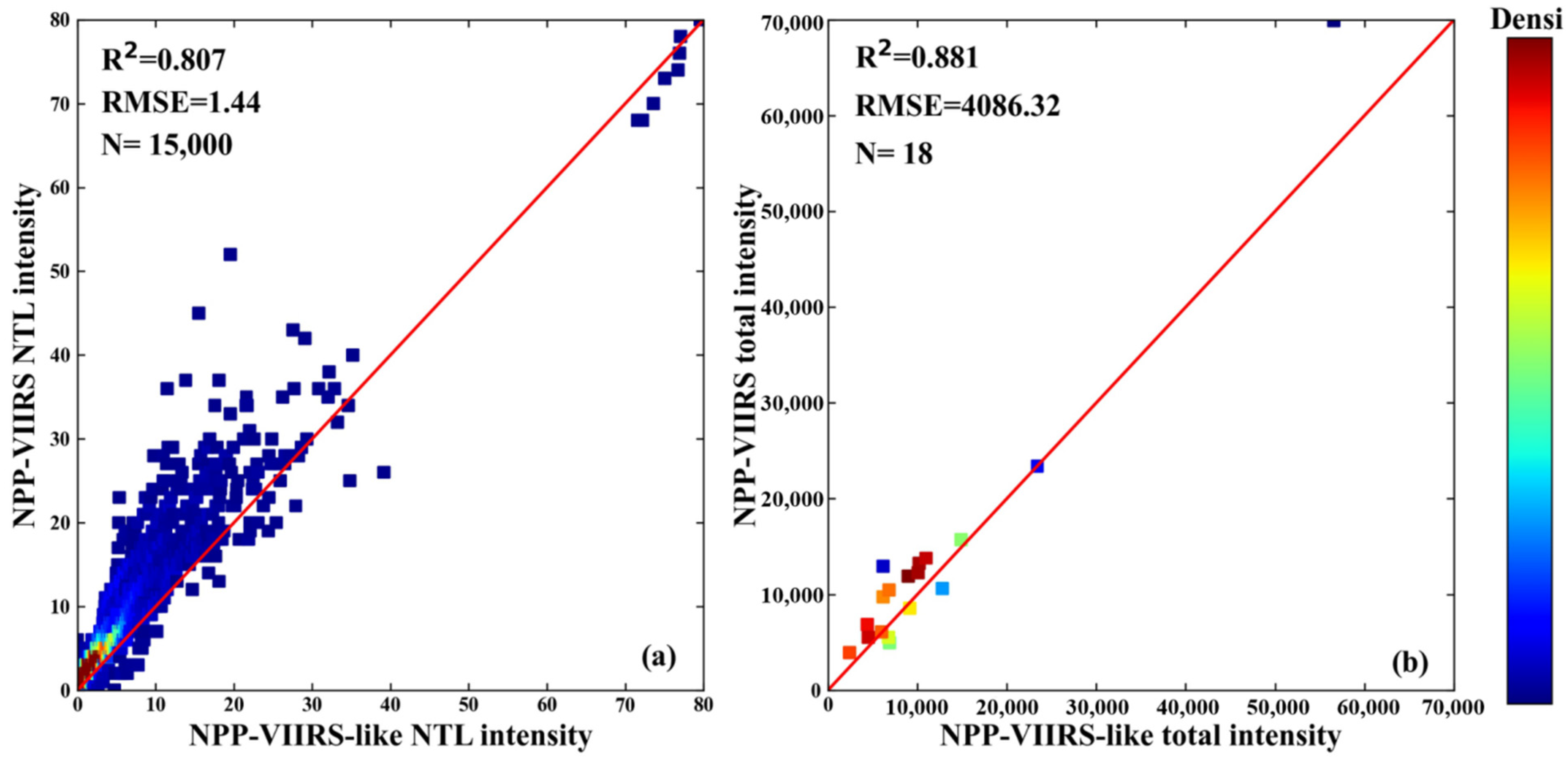
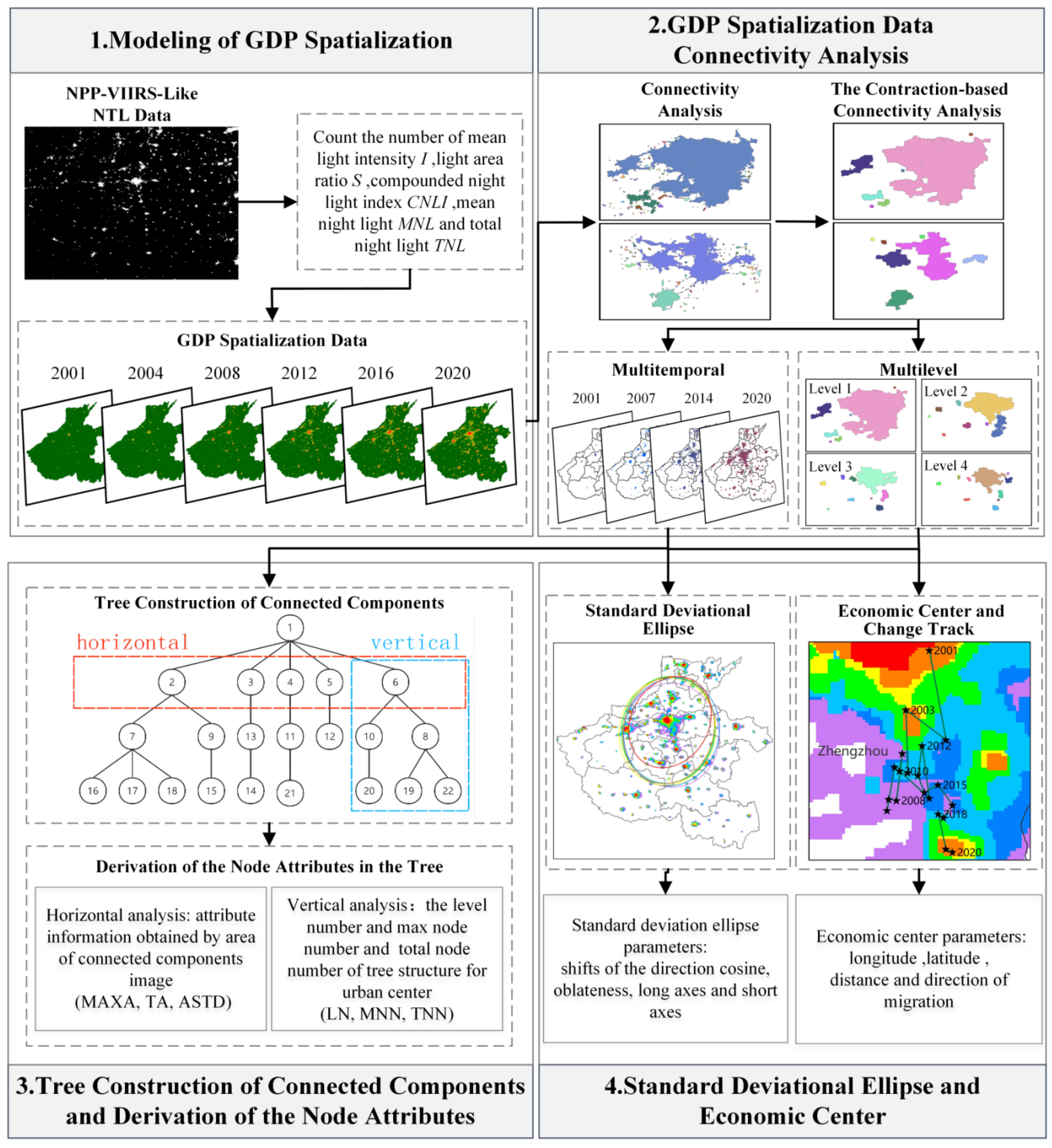
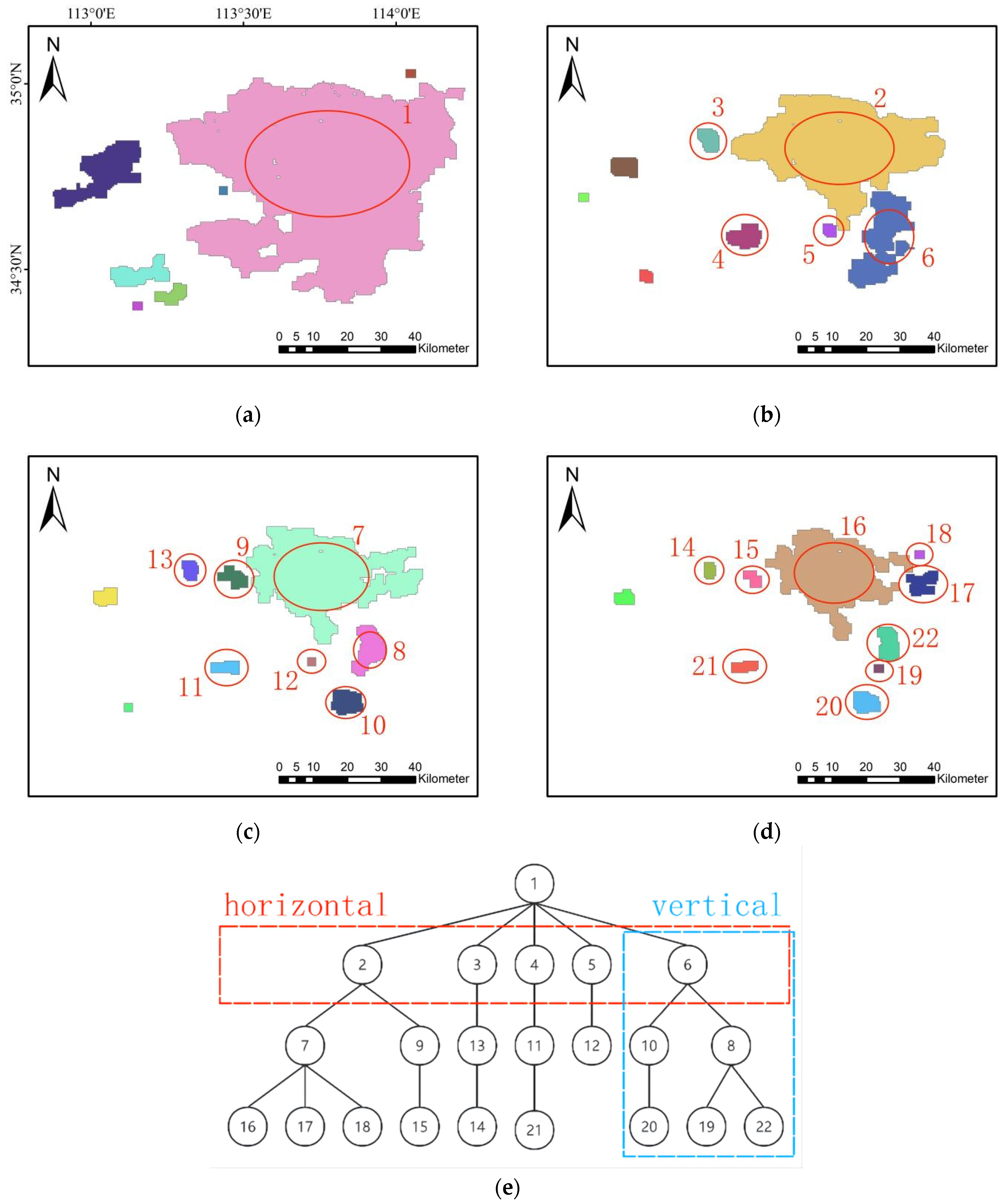
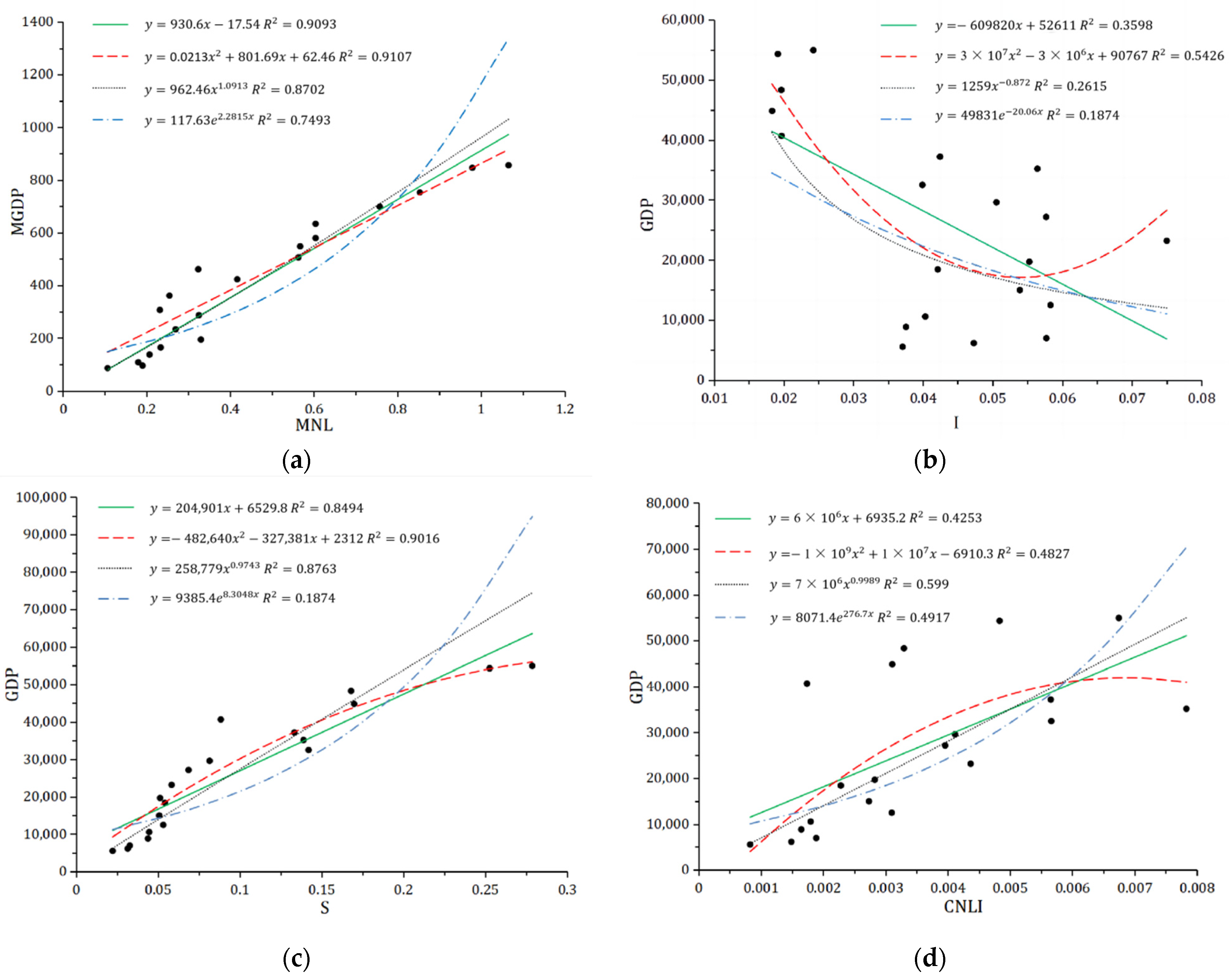
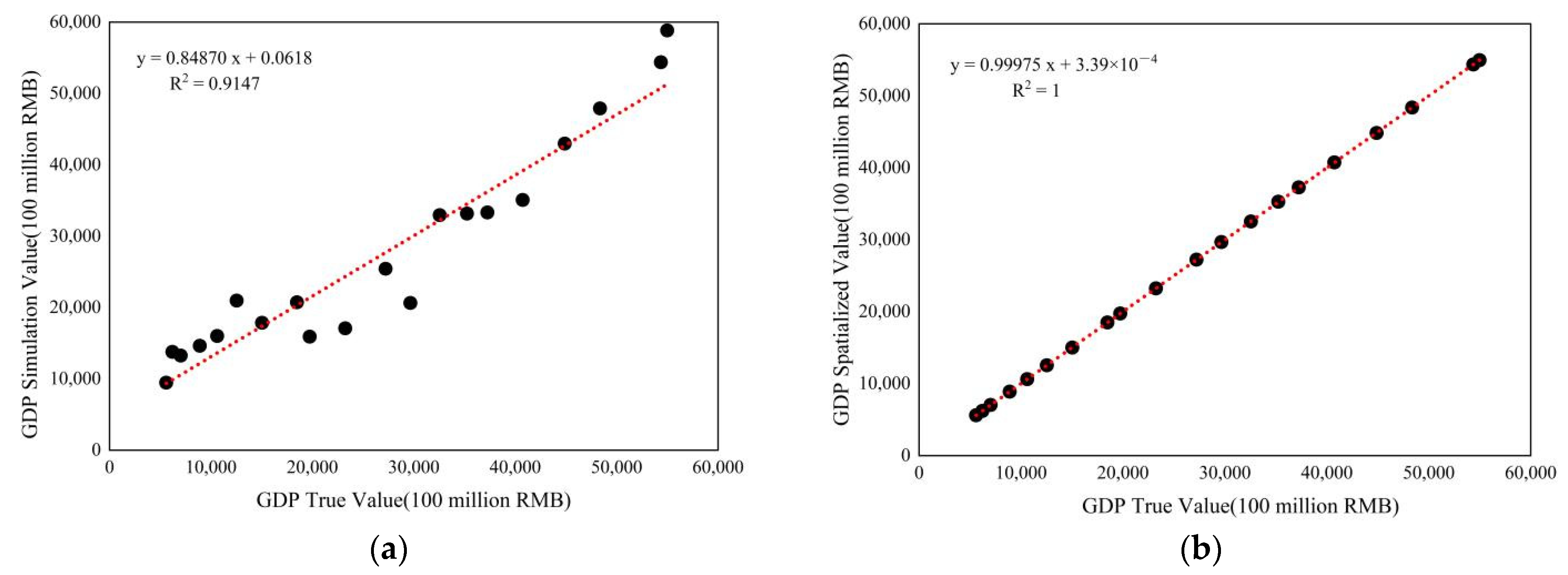
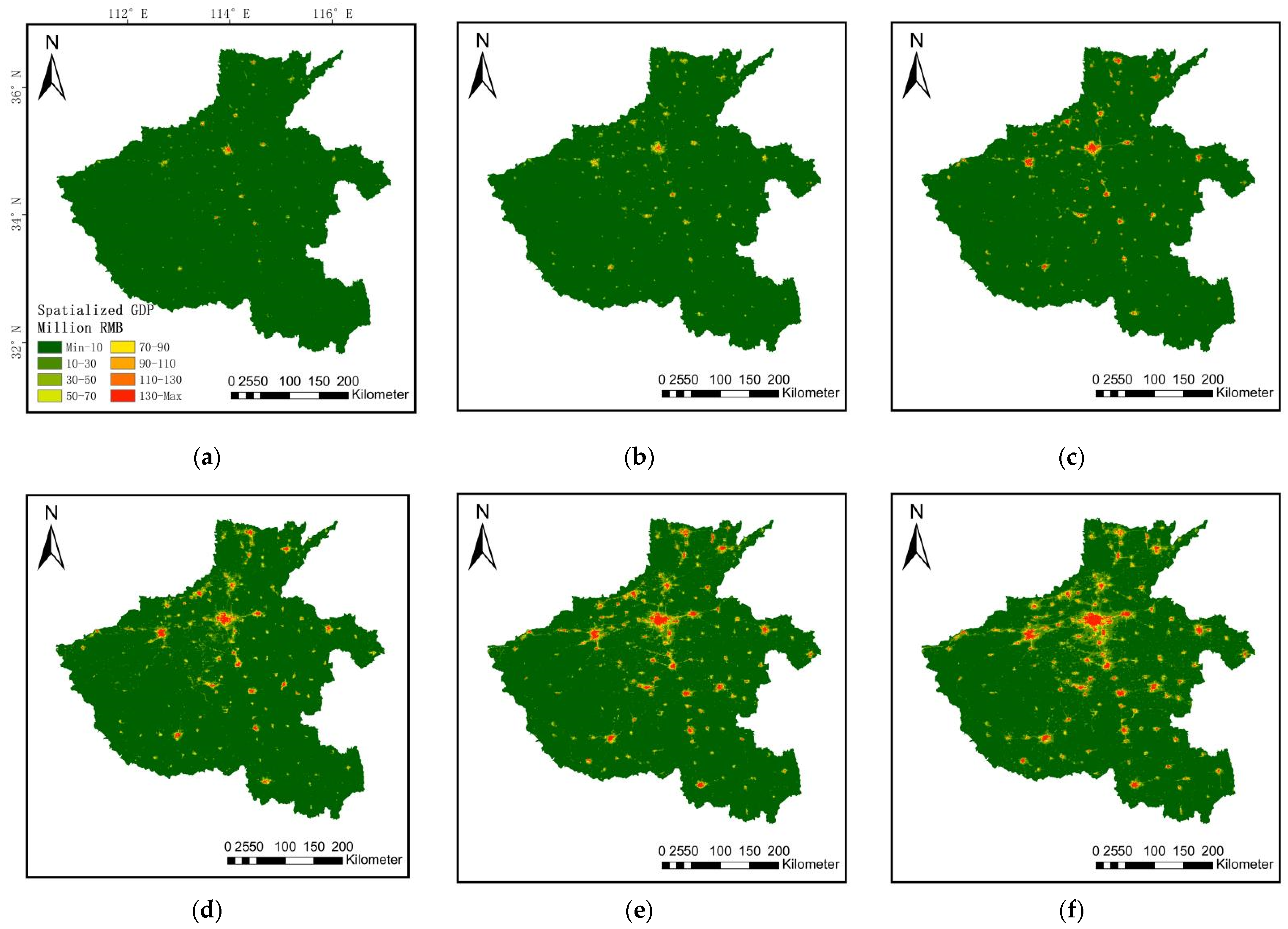
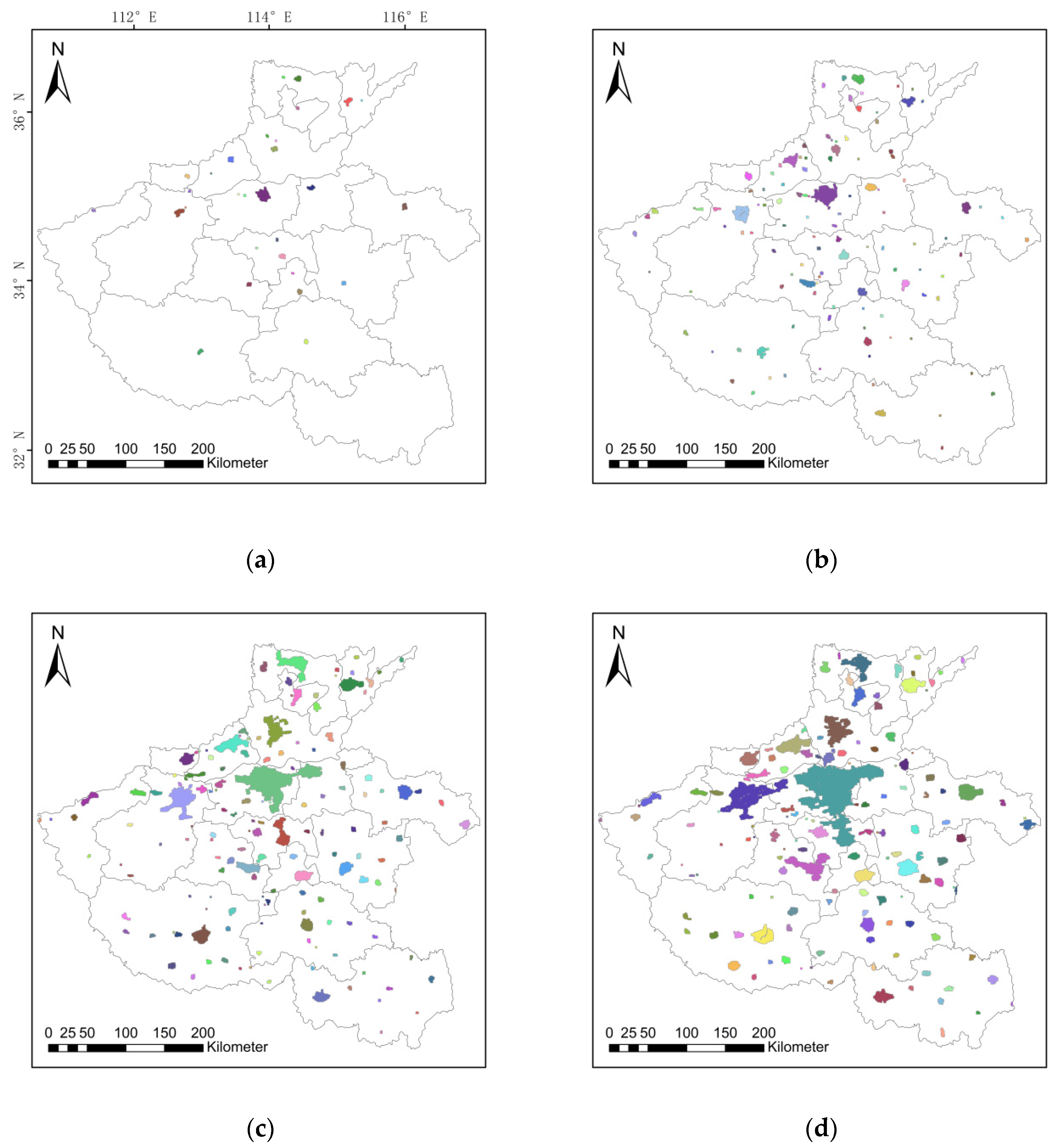
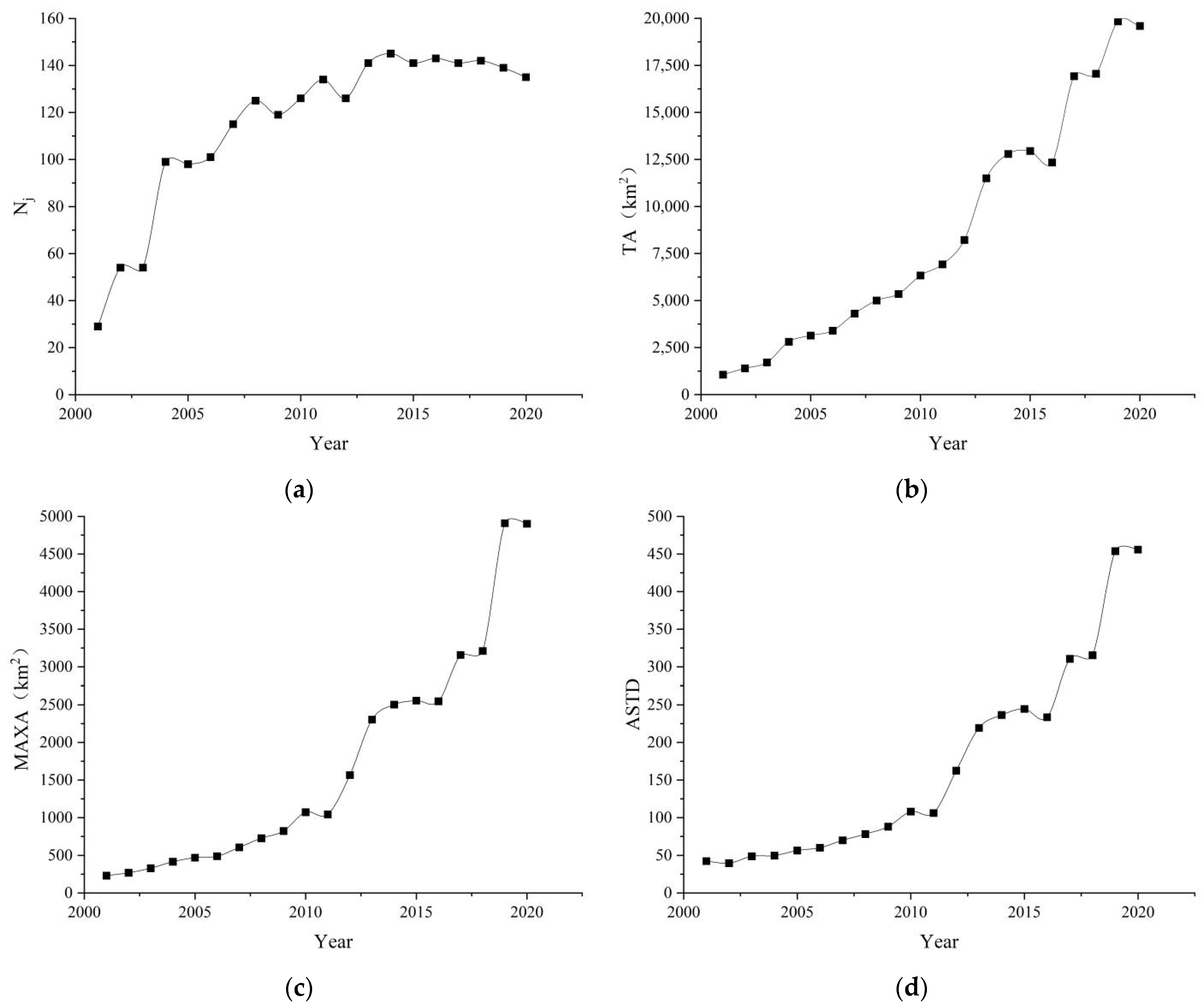
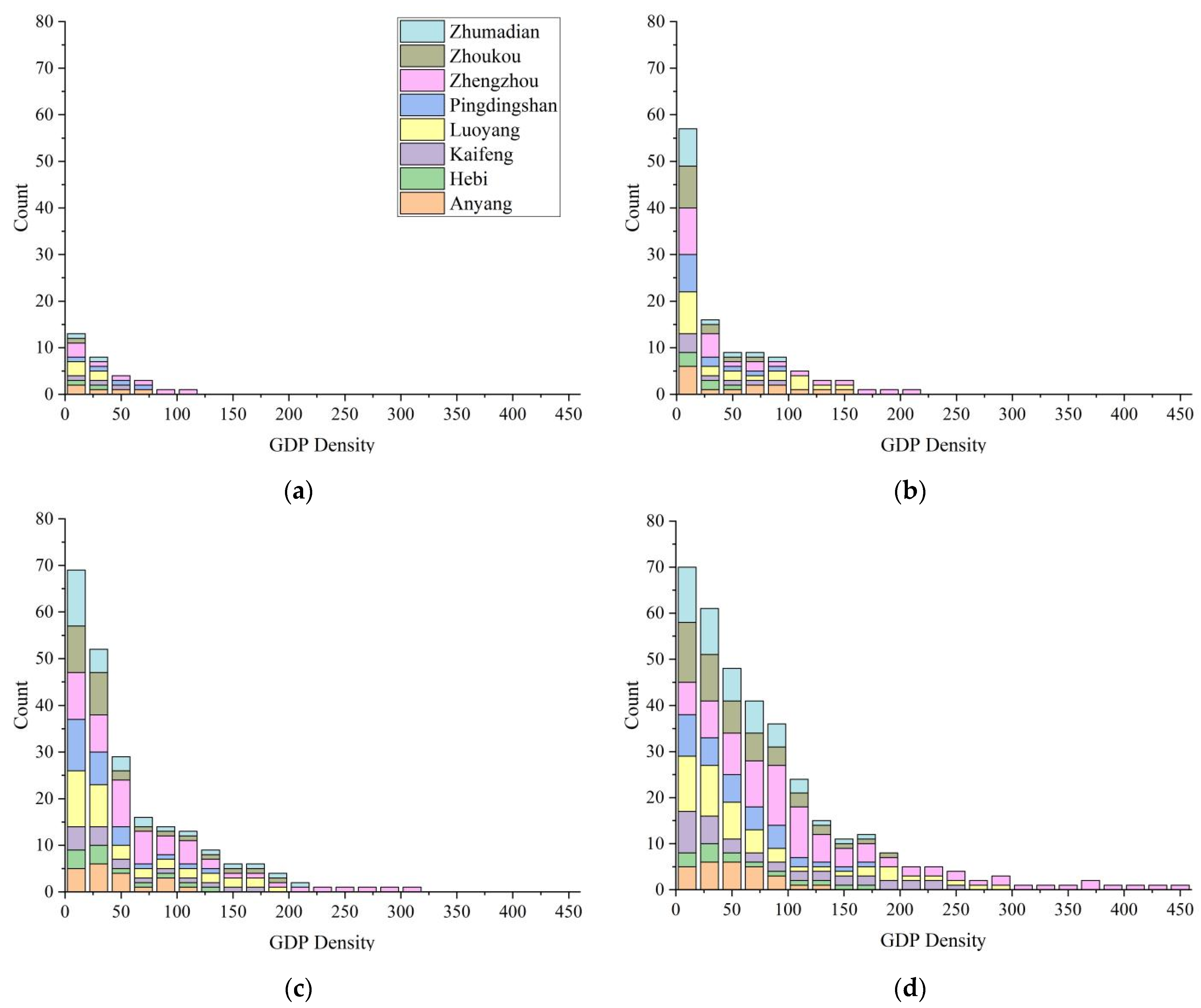
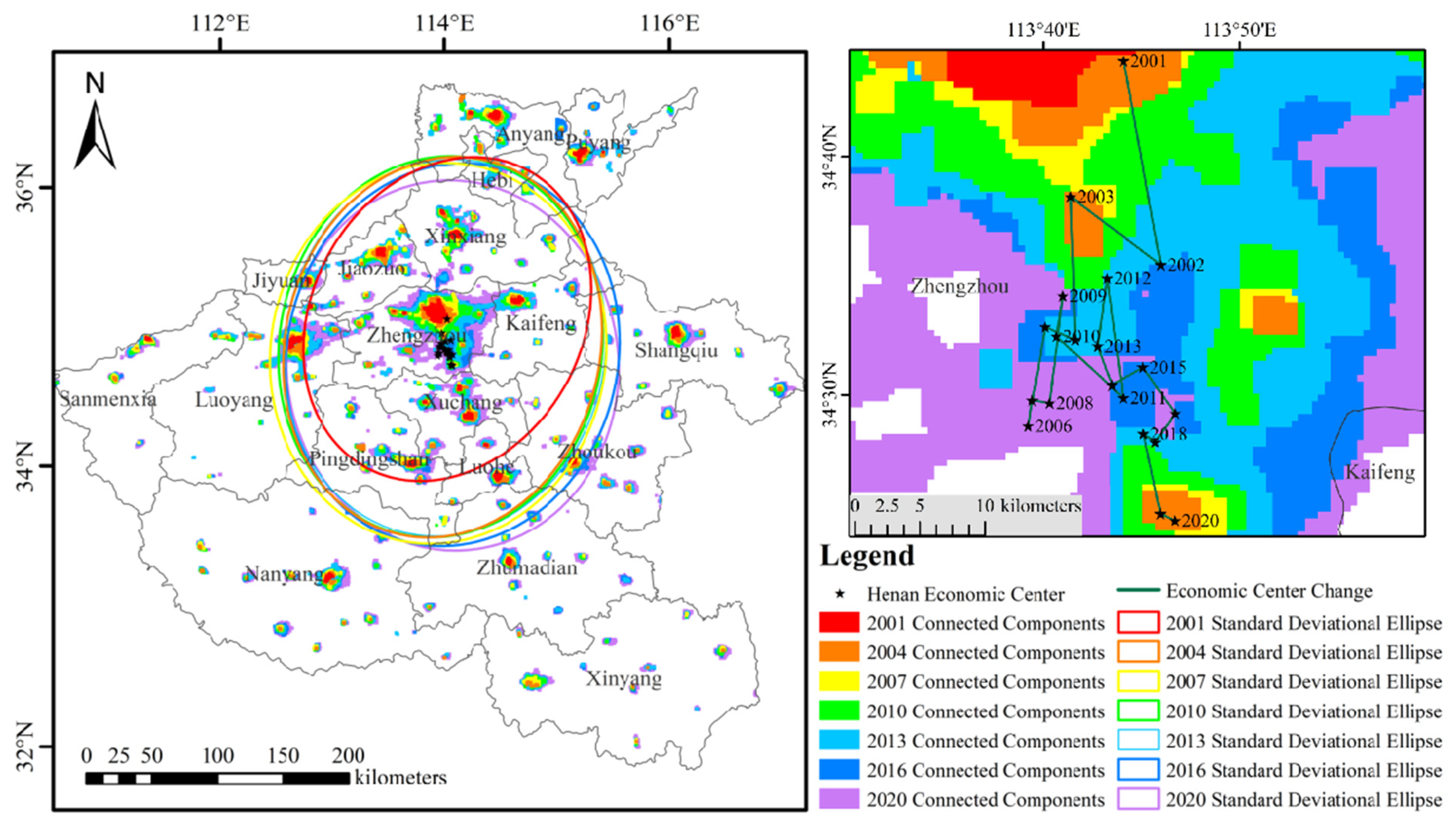
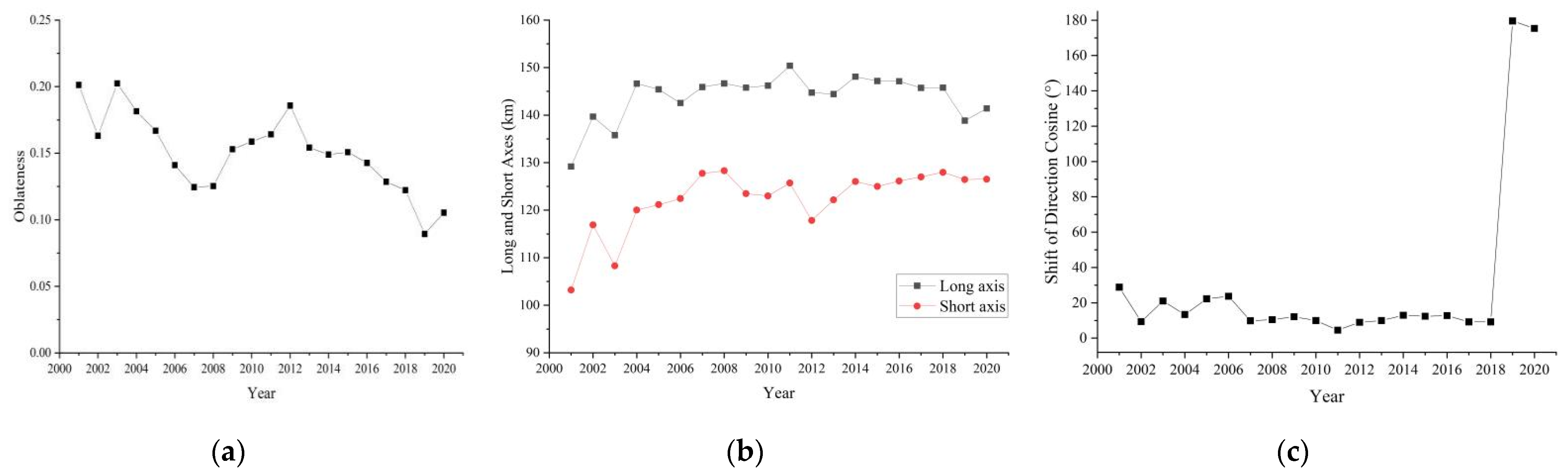
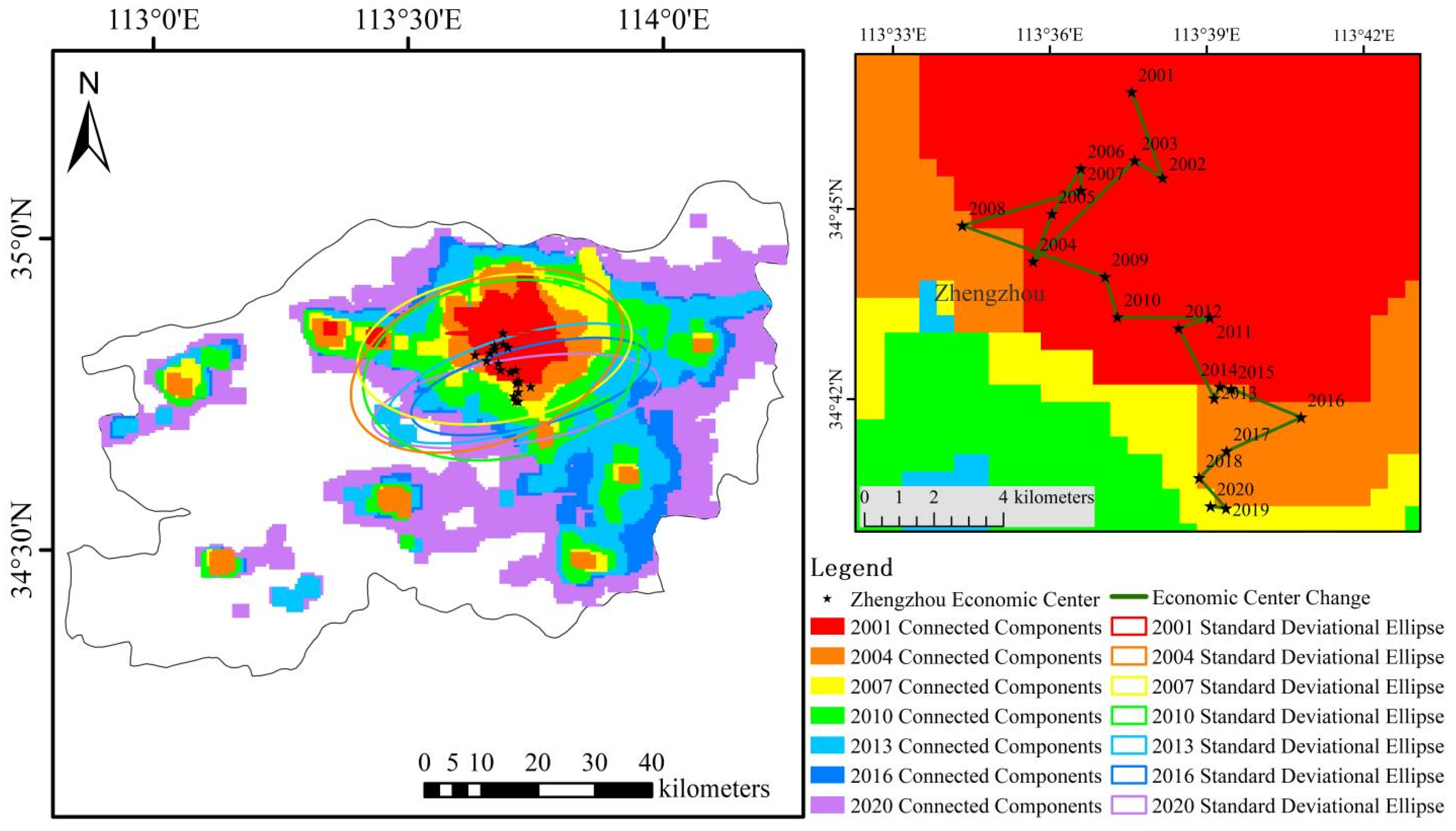
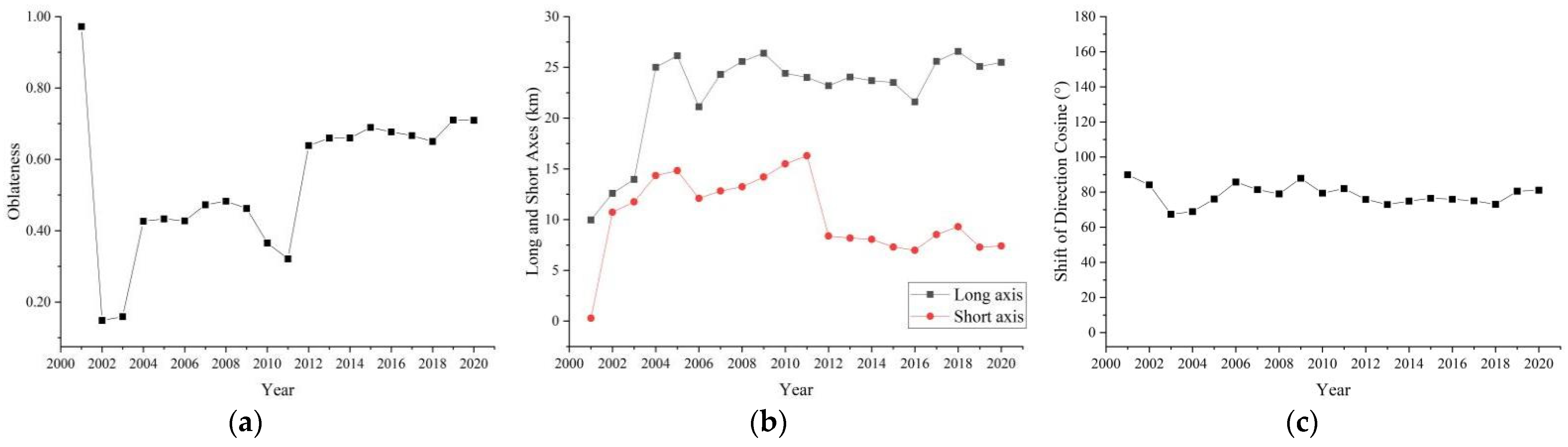
Table 1.
NTL indices and economic parameter list.
| Attribute | Definition |
|---|---|
| The pixel whose gray value is i in the area. | |
| The pixel with the maximum gray value in the area. | |
| The gray value in the area is the number of i pixels. | |
| N | The total number of pixels in the area. |
| The total number of pixels whose gray value is not 0 in the area. | |
| Total nighttime light (TNL) | |
| Mean nighttime light (MNL) | |
| Average relative light intensity (I) | |
| Light area ratio (S) | |
| Compounded nighttime light index (CNLI) | |
| Mean gross domestic product (MGDP) |
Table 2.
City analysis parameter list.
| Attribute | Definition |
|---|---|
| Nj | Nj is the number of connected components at level 1. |
| Maximum area (MAXA) | |
| Total area (TA) | |
| Average area (AVA) | |
| Area standard deviation (ASTD) | |
| Level number (LN) | LN is the level number of a tree structure for the urban center. |
| Maximum node number (MNN) | MNN is the max node number of a tree for the urban center. |
| Total node number (TNN) | TNN is the total node number of a tree for the urban center. |
* ai is the average area of the first node.
Table 3.
Henan Province information from 2001–2020 on the parameters of the economic centers.
| Year | Longitude | Latitude | Migration Distance (km) | Direction |
|---|---|---|---|---|
| 2001 | 113°44′1″ E | 34°42′47″ N | - | - |
| 2002 | 113°44′45″ E | 34°34′1″ N | 15.96 | Southeast |
| 2003 | 113°40′34″ E | 34°37′19″ N | 8.70 | Northwest |
| 2004 | 113°39′59″ E | 34°31′16″ N | 11.01 | Southeast |
| 2005 | 113°38′32″ E | 34°31′57″ N | 2.53 | Northwest |
| 2006 | 113°37′7″ E | 34°27′52″ N | 7.72 | Southwest |
| 2007 | 113°37′27″ E | 34°28′56″ N | 1.98 | Northeast |
| 2008 | 113°38′19″ E | 34°28′44″ N | 1.35 | Southeast |
| 2009 | 113°39′36″ E | 34°33′11″ N | 8.31 | Northeast |
| 2010 | 113°39′3″ E | 34°31′31″ N | 3.14 | Southwest |
| 2011 | 113°42′6″ E | 34°28′37″ N | 7.00 | Southeast |
| 2012 | 113°41′58″ E | 34°33′43″ N | 9.26 | Northwest |
| 2013 | 113°41′6″ E | 34°30′54″ N | 5.27 | Southwest |
| 2014 | 113°41′37″ E | 34°29′12″ N | 3.17 | Southeast |
| 2015 | 113°43′16″ E | 34°29′48″ N | 2.71 | Northeast |
| 2016 | 113°44′39″ E | 34°27′42″ N | 4.34 | Southeast |
| 2017 | 113°43′28″ E | 34°26′36″ N | 2.70 | Southwest |
| 2018 | 113°42′55″ E | 34°27′0″ N | 1.11 | Northwest |
| 2019 | 113°43′20″ E | 34°23′33″ N | 6.30 | Southeast |
| 2020 | 113°44′2″ E | 34°23′11″ N | 1.24 | Southeast |
Table 4.
Zhengzhou information from 2001–2020 on the parameters of the economic center.
| Year | Longitude | Latitude | Migration Distance (km) | Direction |
|---|---|---|---|---|
| 2001 | 113°37′29″ E | 34°46′22″ N | - | - |
| 2002 | 113°37′54″ E | 34°44′57″ N | 2.63 | Southeast |
| 2003 | 113°37′24″ E | 34°45′17″ N | 0.95 | Northwest |
| 2004 | 113°35′15″ E | 34°43′52″ N | 4.13 | Southwest |
| 2005 | 113°35′42″ E | 34°44′35″ N | 1.48 | Northeast |
| 2006 | 113°36′21″ E | 34°45′15″ N | 1.56 | Northeast |
| 2007 | 113°36′18″ E | 34°44′54″ N | 0.64 | Southeast |
| 2008 | 113°33′58″ E | 34°44′33″ N | 3.56 | Southwest |
| 2009 | 113°36′35″ E | 34°43′30″ N | 4.37 | Southeast |
| 2010 | 113°36′44″ E | 34°42′50″ N | 1.22 | Southeast |
| 2011 | 113°38′30″ E | 34°42′40″ N | 2.67 | Southeast |
| 2012 | 113°37′53″ E | 34°42′33″ N | 0.95 | Southwest |
| 2013 | 113°38′25″ E | 34°41′23″ N | 2.27 | Southeast |
| 2014 | 113°38′33″ E | 34°41′33″ N | 0.37 | Northeast |
| 2015 | 113°38′46″ E | 34°41′30″ N | 0.34 | Southeast |
| 2016 | 113°40′2″ E | 34°40′56″ N | 2.17 | Southeast |
| 2017 | 113°38′33″ E | 34°40′32″ N | 2.36 | Southwest |
| 2018 | 113°37′58″ E | 34°40′9″ N | 1.11 | Southwest |
| 2019 | 113°38′25″ E | 34°39′38″ N | 1.17 | Southeast |
| 2020 | 113°38′7″ E | 34°39′42″ N | 0.45 | Northwest |
Disclaimer/Publisher’s Note: The statements, opinions and data contained in all publications are solely those of the individual author(s) and contributor(s) and not of MDPI and/or the editor(s). MDPI and/or the editor(s) disclaim responsibility for any injury to people or property resulting from any ideas, methods, instructions or products referred to in the content. |
© 2023 by the authors. Licensee MDPI, Basel, Switzerland. This article is an open access article distributed under the terms and conditions of the Creative Commons Attribution (CC BY) license (https://creativecommons.org/licenses/by/4.0/).
Share and Cite
MDPI and ACS Style
Zhao, Z.; Tang, X.; Wang, C.; Cheng, G.; Ma, C.; Wang, H.; Sun, B. Analysis of the Spatial and Temporal Evolution of the GDP in Henan Province Based on Nighttime Light Data. Remote Sens. 2023, 15, 716. https://doi.org/10.3390/rs15030716
AMA Style
Zhao Z, Tang X, Wang C, Cheng G, Ma C, Wang H, Sun B. Analysis of the Spatial and Temporal Evolution of the GDP in Henan Province Based on Nighttime Light Data. Remote Sensing. 2023; 15(3):716. https://doi.org/10.3390/rs15030716
Chicago/Turabian StyleZhao, Zongze, Xiaojie Tang, Cheng Wang, Gang Cheng, Chao Ma, Hongtao Wang, and Bingke Sun. 2023. "Analysis of the Spatial and Temporal Evolution of the GDP in Henan Province Based on Nighttime Light Data" Remote Sensing 15, no. 3: 716. https://doi.org/10.3390/rs15030716
Note that from the first issue of 2016, this journal uses article numbers instead of page numbers. See further details here.