
Mapping Cropland Abandonment in Mountainous Areas in China Using the Google Earth Engine Platform

1
Department of Land Management, Zhejiang University, Hangzhou 310058, China
2
Sichuan Institute of Land Science and Technology, Chengdu 610065, China
*
Author to whom correspondence should be addressed.
Remote Sens. 2023, 15(4), 1145; https://doi.org/10.3390/rs15041145
Submission received: 22 November 2022
/
Revised: 25 January 2023
/
Accepted: 16 February 2023
/
Published: 20 February 2023
(This article belongs to the Special Issue Remote Sensing of Land Use and Land Change with Google Earth Engine)
Abstract
:Knowledge about the spatial-temporal pattern of cropland abandonment is the premise for the management of abandoned croplands. Traditional mapping approaches of abandoned croplands usually utilize a multi-date classification-based land cover change trajectory. It requires quality training samples for land cover classification at each epoch, which is challenging in regions of smallholder agriculture in the absence of high-resolution imagery. Facing these challenges, a theoretical model is proposed to recognize abandoned croplands based on post-abandonment secondary succession. It applies the continuous change detection and classification (CCDC) temporal segmentation algorithm to Landsat time series (1986~2021) to obtain disjoint segments, representing croplands’ status. The post-abandonment secondary succession showing a greening trend is recognized using NDVI-based harmonic analysis, so as to capture its preceding abandonment. This algorithm is applied to a mountainous area in southwest China, where cropland abandonments are widespread. Validation based on stratified random samples referenced by a vegetation index time series and satellite images shows that the detected abandoned croplands have user accuracy, producer accuracy and an F1 score ranging from 43% to 71%, with variation among abandonment year. The study area has a potential cropland extent of 22,294 km2, within which 9252 km2 of the cropland was abandoned. The three peak years of abandonment were 1994, 2000, and 2011. The algorithm is suitable to be applied to large-scale mapping due to its automatic manner.
1. Introduction
Cropland, a primary food source, is the foundation of the livelihood and development of human society. Exponential population increase demands growing food supplies, leading to cropland expansion. The first two decades of the 21st century have experienced a 27% increase in the global population (United Nations World Population Prospects 2019), while cropland increased by 9% [1]. Meanwhile, cropland abandonment is occurring worldwide due to various reasons. For example, in Russia (Soviet Union), it was induced by the collapse of socialism [2]. China, one of the most populated countries globally, struggles to feed 21% of the world population with 9% of the world’s cropland. Even though productivity has increased through intensification and other forms of food, the cropland area is still expected to be increased for the rapid growth of population [3]. The recent seventh national census in China reveals that the Chinese population has increased by 72.06 million over the past ten years. The shrinkage of cropland area per capita makes cropland protection a high priority. After passing the Lewis turning point [4], however, the rising wage of migrant workers resulted in the marginalization of cropland land, which is evidenced by a widespread cropland abandonment phenomenon [5,6,7]. It has been witnessed in the mountainous and hilly areas of the middle and upper reaches of the Yangtze River [8]. How to make full use of these abandoned croplands is particularly critical for food security, climate change mitigation and biodiversity conservation, yet monitoring these abandoned croplands remains a challenge in mountainous areas of China, where smallholder croplands are highly fragmented [9].
Cropland abandonment, one type of land cover change, refers to the cessation of cultivation of cropland over five consecutive years [10]. After abandonment, the original cropland gradually changes to bare land, grassland, shrubland, or forest, depending on the duration of abandonment and local climatic conditions [11]. Remote sensing technology can efficiently obtain synoptic land cover information and change through Earth-observing satellites. Mapping approaches in the existing literature, based on how the trajectory of Landsat time series is classified, can be divided into two categories: multi-date classification approach and hypothesized trajectory approach [12].
Multi-date classification approaches use machine learning algorithms to obtain a series of land cover maps, which are stacked to form a land cover change trajectory [2,13,14,15]. These approaches have two main limitations: (1) Collecting quality training samples for training supervised machine learning models is time- and labour-consuming, and requires local and expert knowledge. In most cases, Landsat imagery is the only source of reference to collect samples, and therefore mapping historic abandoned croplands in smallholder agricultural regions is particularly challenging. (2) Classification errors in individual land cover maps are compounded in the formed land cover change trajectories, which have a low spatial-temporal consistency.
Temporal generalization techniques are proposed to reduce the cost of training sample collection, which commonly use temporally stable features [16,17] or use temporally invariant samples [18], so that training samples can be reused across years. However, it is difficult to obtain temporally stable features from unevenly distributed imagery archives where early observations are far more scarce than recent observations [19].
The sources of non-commercial satellite images mainly fall into three types: (1) hyper-temporal MODIS [14,20], (2) the high spatial resolution Sentinel-2 [9,13], and (3) long time-span Landsat [15,21,22]. MODIS is suitable for mapping the abandonment of large-scale farms in Eastern Europe, but less suitable for mapping scattered and smallholder croplands which only occupy a tiny fraction of the MODIS pixel (250/500/1000 m, depending on bands). Sentinel-2 is suitable for scattered and small-scale cropland, but its short historical image archive does not allow the mapping of croplands abandoned before its launch [23]. Landsat data, with the longest historical records and relatively high spatial resolution, are the best data sources for monitoring the long-term abandonment of cropland in a fragmented agricultural landscape [24]. However, the sparse time series of Landsat observation makes valid observation unevenly distributed in space and time, which is aggravated by clouds and the scan line corrector failure of Landsat-7. An image compositing strategy is routinely adopted to fill the void of images. Apart from a simple compositing strategy such as median and mean compositing, a sophisticated compositing strategy uses a set of rules to select the optimal pixels to synthesize the image of the nominal year in terms of the temporal distance to vegetation growing season, the spatial distance to the nearest cloud, and so on [25]. However, voids and gaps remain in some regions where clouds are persistent, and in some years there are few images acquired. Observations that are acquired beyond the vegetation growing season and the nominal year have to be used instead. Thus, two disadvantages of the image compositing strategy make it less suitable in cropland abandonment mapping: (1) the obscuration of the date of land cover conversion and (2) the loss of phenology information, which is conducive to discriminating among different vegetation types.
In recent years, some time series based change detection algorithms have been developed to identify land cover change and its change date, including LandTrendr [26,27], Vegetation Change Tracker (VCT) [28], Time-Weighted Dynamic Time Warping for Satellite Image Time Series Analysis [29], Breaks For Additive Seasonal and Trend [30], and Continuous Change Detection and Classification (CCDC) [31]. These algorithms detect changes in the trend of the time series, so the influence of noise in the time series is minimized and the temporal consistency is enhanced. At first, they were primarily used in monitoring forest disturbances and their recovery. Their good performance in monitoring vegetation status extends to applications that monitor impervious surface change in built-up areas [32] and cropland abandonment [11,33].
Facing limitations of multi-date land cover classification-based algorithms and recent developments in time series change detection algorithms, this study aims to propose an automatic mapping algorithm which avoids great human intervention in training sample collection. Specifically, the utilization history of croplands is separated into several stages using CCDC temporal segmentation. The phenology information of each stage is fitted using a harmonic function and normalized differenced vegetation index (NDVI) [34] to extract the overall trend component, which is used to classify the status of cropland, either in use or abandonment, since phenology trajectories differ between abandoned and active croplands [9,14,18].
2. Materials and Methods
2.1. Study Area
Sichuan province primarily comprises, after abandonment, the original cropland mountainous counties, and is swept by a cropland abandonment phenomenon. A recent survey shows that the total extent of abandoned croplands in Chinese mountainous counties between 2000 and 2010 is estimated at 98,000 km2; in total, about 28% of the croplands in mountainous counties were abandoned, including croplands converted in the Grain for Green Programme [35]. Our study selects one Landsat footprint whose Landsat World Reference System-2 identifier is 129/40 (Path/Row) as the study area, covering the southeast corner of Sichuan Province. The terrain of the study region can be divided into the southwest mountainous region, where the highest elevation above sea level is 3998 m, and the northeast hilly region (Figure 1). The study area has a subtropical monsoon climate, with an average annual temperature of 17 °C and an annual rainfall of 1050–1168 mm. It has four distinct seasons, with rain and heat occurring during the same season, early warming in spring, high humidity in summer, and frequent rain in autumn. The natural vegetation is mainly evergreen and broad-leaved forest.
2.2. Data
This study mainly uses two datasets: cropland products and Landsat image collection. The former is used to obtain potential historical cropland extent, while the latter is used to retrieve vegetation dynamics over those croplands.
2.2.1. Cropland Products
To comprehensively analyse the spatial-temporal process of cropland abandonment, all land that used to be cropland since 1990s should be included for subsequent analysis. Some land cover datasets and cropland maps of fine spatial resolution have been released recently, delineating cropland distribution in mountainous and hilly regions. Some representative products are selected to obtain potential historical cropland extent, and their metadata and references are listed in Table 1 These landcover and cropland products are not perfect. It is their difference in accuracy [36] that makes the union of cropland products a necessity to reduce the omission error of croplands. That is, one site is considered to be cropland if it is flagged as cropland in any of these products.
For comprehensive information, refer to the references listed in the right-most column of Table 1. A brief description of these products follows:
- (1)
- GlobeLand30, the world’s first 30 m land cover product, adopts Pixel- and Object-based methods with Knowledge (POK). It consists of land cover maps for three epochs: 2000, 2010, and 2020.
- (2)
- The China Land Cover Dataset (CLCD), produced with Google Earth Engine, is an annually based land cover map spanning 1990 to 2019.
- (3)
- Finer Resolution Observation and Monitoring of Global Land Cover at 10 m (FROM-GLC10) is the world’s first 10 m land cover product produced, from which existing training samples, built for previous land cover maps (FROM_GLC30), are reused and applied to Sentinel-2 images of 2017.
- (4)
- The land cover map of 2015, GLC_FCS30, is produced using a global spatial-temporal spectra library.
- (5)
- The Cropland_Potapov product has mapped global cropland since 2003. It has a minimum map unit of 0.5 ha, so fragmented croplands smaller than 0.5 ha are omitted.
- (6)
- The China Terrace Map of 2018, produced from Landsat-8 data and digital elevation model data, mapped terrace cropland in China.
2.2.2. Landsat
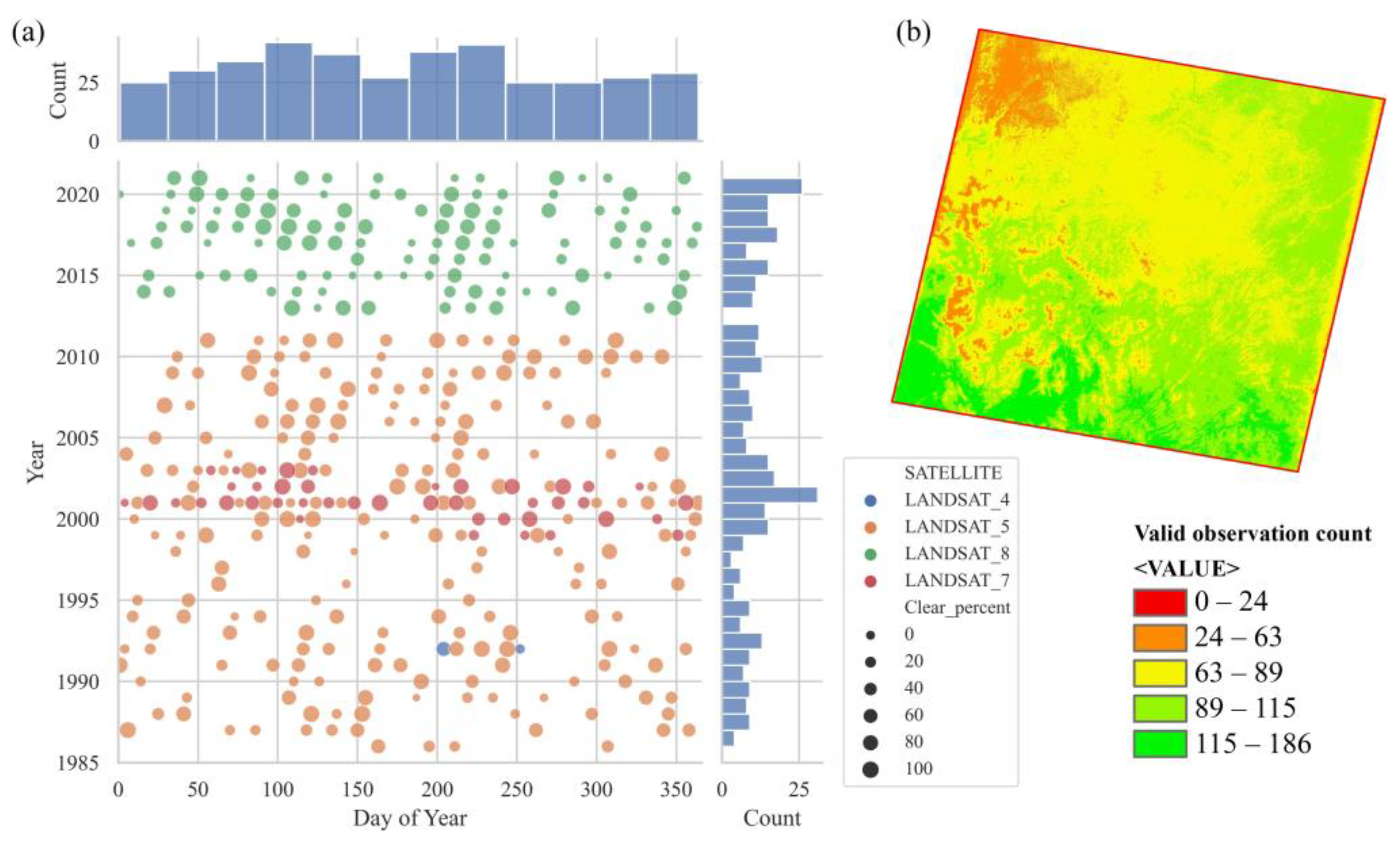
This study aims to retrieve the occurrence of cropland abandonment between 1990 and 2020. Landsat surface reflectance Tier 1 images acquired at this footprint (WRS Path: 129 Row: 40), except for the Landsat-7 images acquired after scan line corrector failure in 31 May 2003, are selected, totalling 380 images. The temporal distribution of these images is illustrated in Figure 2a, where the colour and size of dots denote the satellites and the clear pixel percentage of images, respectively. The marginal x-axis shows the aggregated distribution by day of the year. It is worth noting that images acquired during the peak vegetation period (around the 170th day of the year) are fewer than in neighbouring months, which can be explained by the synchronous timing of the rainy and hot seasons. The marginal y-axis shows the aggregated distribution by year. A very uneven distribution across the years is observed. In general, the number of images per year features an upward trend from 1986 to 2021. The former half of the period before 2001 has fewer images, while the latter half after 2012 has more images, except for 2012. The sparse image time series is obscured by persistent clouds during the rainy season, making the distribution of valid observations extremely uneven. As shown in Figure 2b, the maximum and minimum valid observations are 186 and 0, respectively. To facilitate visual inspection, the values of valid observations are divided into five classes by the Natural Breaks algorithm of ArcMap 10.7. The lowest two classes are mainly distributed in the northwest corner, urbanized region, and southwest corner, mountainous region. The highest class is concentrated in the south.
2.3. Methods
Currently, it is a challenge to identify the time and type of land cover conversion. To overcome these challenges, this study proposes a four-step algorithm (Figure 3). First, the potential historical cropland extent is obtained as the union of existing cropland products, because our aim is to minimize the omission error of croplands rather than commission error. Second, the 36-year observational time series of croplands is segmented by the CCDC temporal segmentation algorithm to discrete periods representing different stages of vegetation status. Third, the overall trend and segmented change are retrieved using a normalized difference vegetation index (NDVI [34]) based harmonic function and are used as input to a simple decision tree to identify abandoned croplands. Finally, we validate the results on stratified random sampling by referencing the vegetation index time series and satellite images (Area-weighted estimation …). Apart from the last step, which is conducted on a local computer, the first three steps are conducted using the Google Earth Engine (GEE) platform [42].
2.3.1. Cropland Mosaicking
Limited by algorithms and data sources, every land cover product has an omission error [43]. To reduce the omission error of croplands, the potential historical cropland extents are extracted as the union of croplands of multiple land cover products and cropland products. As this study focuses on vegetation succession over croplands, croplands converted to built-up areas or water bodies due to urbanization and lake (river) expansion are excluded using GlobeLand30 land cover products of 2000, 2010, and 2020 [37].
2.3.2. Temporal Segmentation
Using all available observations, the time series temporal segmentation algorithm, CCDC [31], is sensitive to more land cover change types and is more accurate in retrieving the change date compared with former algorithms, which are built on an annual-basis time series of a single indicator (e.g., LandTrend [26], VCT [28]). Following [44], it is suggested to use all bands of Landsat images, six spectral bands plus one thermal band, to detect change using the harmonic function (Equation (1)):
where:
- x Julian date;
- i the i-th Landsat band;
- k the number of Landsat band;the coefficient for overall value for the ith Landsat Band;
- the coefficients for intra-annual change for the ith Landsat Band;
- the coefficient for inter-annual change for the ith Landsat Band;
- the k-th breakpoint;
- the predicted value for the ith Landsat Band at Julian date x based on OLS fitting.
If land cover change does not occur, the observed value should fall within the range of the predicted value plus or minus three times the average root-mean-square error; otherwise, change occurs [31]. As transient noises (e.g., undetected cloud) can be detected as pseudo-change, this method requires six consecutive observed values to fall beyond the predicted range to flag change. This change detection condition is defined in Equation (2):
where is the observed value for the i-th Landsat Band at Julian date x. The same parameters used in the previous equation are not described here.
Two parameters, minObservation and minNumOfYearScaler, are set with relatively large values to reduce sensitivity to transient phenology disturbance, such as fallow and crop rotation. Other parameters are listed in Table 2, together with their values and descriptions.
2.3.3. Trajectory Classification
After abandonment, croplands experience complicated vegetation succession [45]. Conventional land cover classification algorithms, which rely heavily on spectral features, are sensitive to phenology variation. For example, the spectral characteristics of crops differ greatly in the growing and senescence stages, which challenges the conventional spectra-based algorithms. Contrary to the volatile seasonality component, the interannual trend component of phenology is steady, so it is used in this study to identify abandoned cropland.
The harmonic function indicated by Equation (4) is used to fit the NDVI (Equation (3) [34]) time series for each segment to extract phenology information. The phenology information is decomposed into an interannual trend component, an intra-annual seasonality component, and a residual component. The trend component and seasonality component can clearly discriminate among vegetation types. For example, the green leaf cover of evergreen woody vegetation has a weak seasonality component superimposed on a high trend component, contrary to herbaceous vegetation (e.g., crops), which has a strong seasonality component superimposed on a low trend component [46].
Here, is the predicted value at time t; (slope ∗ t + intercept) is the trend component of phenology; and the trigonometric functions represent the seasonality component where are seasonal harmonic coefficients of n-th order. The highest frequency, N, is commonly set to 3. As N increases, a seasonality component of higher frequency is added to the harmonic function, allowing it to fit a more complex curve; meanwhile, more observations are required to determine additional harmonic coefficients. For example, at least four valid observations are needed to solve the equation system when N equals 1. The N value is automatically determined by the number of valid observations of segments.
Different stages represent different vegetation states, each with distinct phenology information. Figure 4 shows the raw NDVI values and fitted harmonic functions over a cropland that was abandoned in 2006. Its 36-year dynamic is divided by a CCDC algorithm into four stages. The first two stages are active cropland under regular cultivation, whose trend component is constant; the third is the vegetation succession stage, whose trend component increased from lower values, compared with its previous stage, to higher values; the fourth is the evergreen vegetation stage, whose overall value of trend component is substantially higher than active cropland stages.
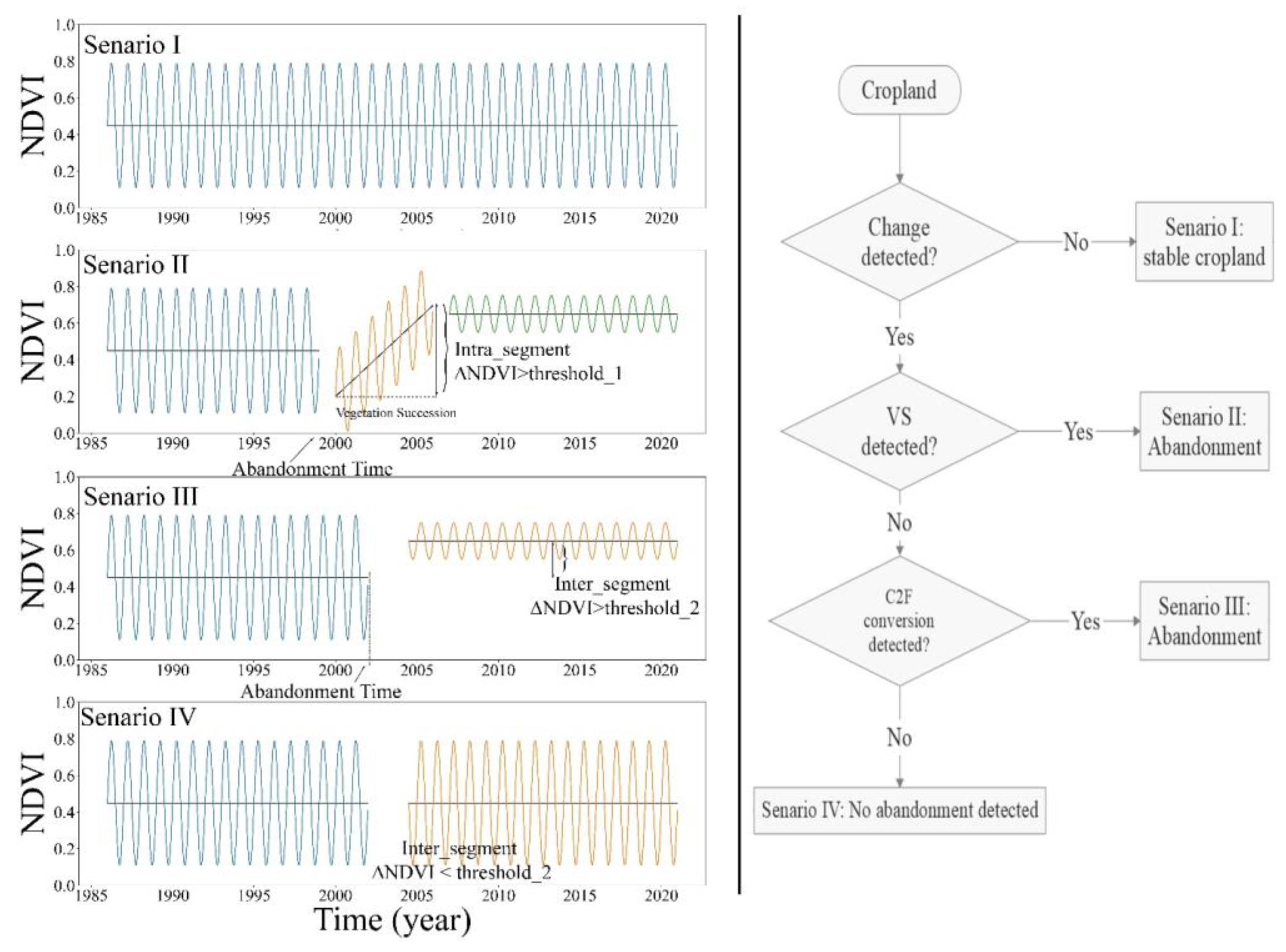
Given the distinct pattern of trend component changes after croplands are abandoned, this study advances a theoretical model and an associated decision tree model to identify abandoned croplands (Figure 5). Cropland evolution is categorized into four scenarios, of which two correspond to abandonment. In scenario I, croplands are constantly under cultivation so no change is detected by the CCDC algorithm. In scenario II, the cropland is abandoned and gradually encroached upon by natural vegetation. Plenty of valid observations allows the CCDC algorithm to detect all three stages: active cropland stage, vegetation succession stage, and stable evergreen vegetation stage. However, in most abandonment cases, the complicated and volatile vegetation succession stage is difficult to fit from scarce valid observations, leaving only two stages: before and after abandonment (Scenario III). In scenario IV, change is detected but the phenology information of the latter segment is similar to its previous segment. The difference between scenario I and IV is whether a transient disturbance is detected. In Scenario IV, the cropland experiences one transient disturbance (e.g., flood, wind) in one year, interrupting the stable time series, while the cropland in Scenario I does not experience it. It should be noted that croplands occupied by urbanization are excluded, so that the transformation to urban area is not included in our theoretical model.
It is critical to design rules to classify cropland dynamics into abandonment scenarios (II, III) and non-abandonment scenarios (I, IV). The inner-segment delta overall of NDVI (Equation (5)) is used to identify the vegetation succession stage in scenario II; the inter-segment delta overall of NDVI (Equations (6) and (7)) is used to identify the increase of overall NDVI in Scenario III. A simple decision tree model consisting of these rules is shown in Figure 5. After trajectory classification, the abandonment time can also be obtained, defined as the end time of the segment before abandonment (Figure 5).
Here are the starting and ending times of the segment. The slope and intercept are the coefficients of the fitted phenology function.
The appropriate thresholds in Equations (5) and (6) are determined according to sensitivity analysis with five hundred random samples, representing a trade-off between producer and user accuracy.
2.3.4. Validation
As the ground truth reference cropland abandonment dataset is missing, the derived results are validated against the vegetation index time series, Landsat images, and finer resolution images, if available. Though Very High Resolution (VHR) commercial satellite images applied by manual interpretation can provide an approximate ground truth dataset, they were either too few or of too small coverage in Google Earth before 2010. In the period before 2010, Landsat images are the only source of a reference dataset. Displayed in suitable band combinations to highlight the differences between vegetation types and complemented by a vegetation index time series, Landsat images can provide a reliable reference dataset whose accuracy approximates that derived from a VHR image [47]. In the period after 2010, the abundance of VHR images in Google Earth eases the validation of newly abandoned croplands.
To facilitate the validation procedure, some software and tools are used including Collect Earth [48], Google Earth, Google Earth Engine Platform, and Time Series Viewer (https://parevalo_bu.users.earthengine.app/view/quick-tstools (accessed on 15 February 2023)). Collect Earth is a tool that enables image interpretation through Google Earth in a user-friendly interface, in conjunction with Bing Maps and Google Earth Engine. However, the functionality of inspecting vegetation index time series is weak. To supplement this functionality the Time Series Viewer is used, which can be described as a simple interactive Earth Engine Application that allows the user to explore a series of Landsat observations for any pixel on the globe where such data are available and to select the spectral band and time range to visualize and click on any point in the time series to load the corresponding image into the map viewer [49]. Following [11], the resulting validation is conducted on 400 stratified random samples from a trajectory type map, 100 for each type, to ensure an even distribution and representativeness of samples [50]. The reference result of these samples is obtained with the aid of those software and tools, independently. The agreement is reached if the offset between reference date and algorithm identified date is less than one year, considering the uncertainty in manually interpreted abandonment date, or the sample is labelled as non-abandonment by both. Classification performance is measured by producer accuracy (PA), user accuracy (UA), and F1 score (=2 ∗ PA ∗ UA/(UA + PA)). Due to sample scarcity in some years, these metrics are calculated on a five-year basis (e.g., 2000~2004) to ensure reliability.
3. Results
3.1. Cropland Mosaicking
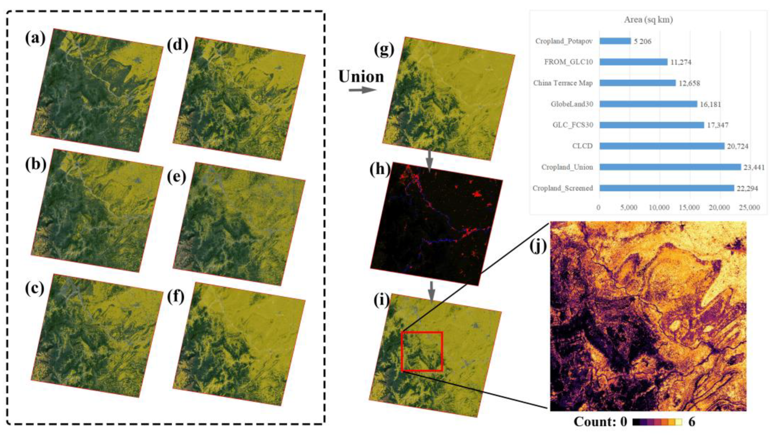
The procedure of cropland mosaicking is illustrated in Figure 6. Cropland area statistics show that Cropland_Potapov has the minimal cropland of 5206 km2 because it excludes fragmented croplands less than 0.5 ha and does not include abandoned croplands which have been non-croplands before 2003. The CLCD has the most cropland, constituting 20,724 km2, likely because it has the longest time span and annual basis. The union of croplands has an area of 23,441 km2. After screening for built-up areas and water bodies it has an area of 22,294 km2, over which we conducted the subsequent analysis.
3.2. Temporal Segmentation
For each cropland pixel, its 36-year record of Landsat observation is divided by the CCDC temporal segmentation algorithms into one (no change detected), two, three, or more segments. As shown in Figure 7, 68.3% of croplands are stable, without change detected; 30.45% showed change, within which 81.8% changed only once; and 1.26% are undetermined due to a scarcity of valid observations and/or complicated land cover dynamics.
3.3. Trajectory Classification
Figure 8 shows the distribution of the intra-segment (Figure 8a) and inter-segment (Figure 8b) delta overall over the start time of the segments. The marginal x-axis shows an aggregated distribution over time. Around 2000, many segments emerged; most had a positive intra-segment delta overall of around 0.18, and a positive inter-segment delta overall of around 0.16. The time frame coincides with the year when the Grain for Green Project pilot started in Sichuan Province, which converted a lot of slope cropland into natural vegetation to reduce soil erosion. The marginal y-axis shows an aggregated distribution by delta overall. Most delta overalls, both inter-segment and intra-segment, have positive values, indicating a large-scale greening trend.
To identify abandoned cropland based on the delta overall values of segments, it is critical to assign suitable values to threshold_1 and threshold_2. Figure 8c,d show the sensitivity analysis on threshold_1 and threshold_2, respectively. As the threshold increases, UA increases while PA decreases, meaning that the omission rate of abandoned cropland increases and the commission rate decreases. To keep a balance between PA and UA, threshold_1 and threshold_2 are both set to 0.1. After the critical thresholds are set, abandoned croplands are identified by the decision tree model.
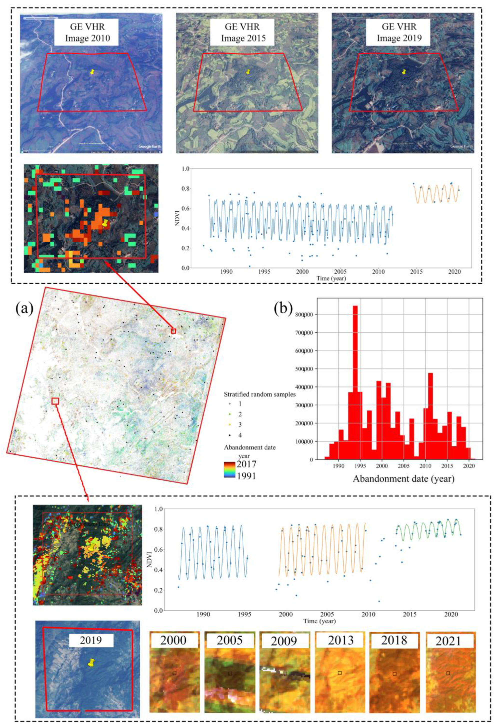
Figure 9 shows where they were, and Figure 10 shows when they occurred. The potential historical cropland extent in the study region was 22,294 km2, within which 9252 km2 of croplands were abandoned according to error-adjusted area estimator [50], leading to an abandonment rate of 41.5%. The three peak years for abandonment were 1994, 2000, and 2011. The spatial distribution of abandonment occurrence is widely dispersed, with a few local clusters. In the 1990s, abandonments occurred mainly in the middle-eastern part of the domain with a few clusters in the north-western corner; in the 2000s, abandonments were clustered in the south-eastern corner; in the 2010s, there were several clusters in the north-west.
3.4. Validation
The four hundred stratified random samples for validation are shown in Figure 8a, in which the abandonment dates over two samples are shown in the upper and bottom images in the dotted squares. The upper sample in the hilly region was estimated to be abandoned in 2012 by our algorithm; the VHR images in Google Earth proved that it was cropland in 2010 but forest in 2015 and 2019. The bottom sample in the mountainous region was estimated to be abandoned in 2009. Due to the lack of VHR images, it is referenced against medium resolution satellite imagery. The annual composited images using images acquired during the growing season prove that it was cropland before 2009 (due to page limitation, only images in 2000, 2005, 2009 are displayed in Figure 10) and a highly vegetated area after 2013.
Our proposed algorithm results in a promising map of abandonment, albeit with variations in accuracy among different classes. The non-abandonment class has PA, UA, and F1 ranging from 62% to 75%, while the abandonment classes range from 43% to 71% with large inter-class variation (Figure 11). The worse harmonic fitting from sparse and irregular Landsat time series in the 1990s provides less reliable phonologic characteristics, which is the main reason for the lower mapping accuracy. The launches of Landsat-7/8 and the shift of acquisition scheme densify the Landsat time series, improving mapping accuracy substantially.
4. Discussion
Mapping abandoned cropland is challenging, especially in regions of smallholder agriculture. In the existing literature, a multi-date classification approach is the mainstream. However, cropland has heterogenous spectral characteristics caused by crop plantation, phenology, and agricultural management practices (e.g., crop rotation, tillage, harvest). After being abandoned, its spectral characteristics change continuously in the post-abandonment secondary succession process. A mixed pixel effect, which is severe in smallholder agricultural regions where cropland fields are smaller than pixel size, brings additional uncertainty in spectral information. Given the difficulty of recognising abandoned croplands from spectral features, additional features are usually used as a complement, including temporal features and spatial features (texture).
4.1. Multi-Date Classification Approach
Classification errors in individual classification, which result from phenology, illumination condition, atmospheric noise and other error sources, are compounded in stacking operation. To reduce error sources, only images acquired during vegetation growing season are selected or de-seasoning methods are applied, which reduces the availability of valid observations. Image compositing, such as temporal aggregation and optimal pixel selection, is utilized to obtain wall-to-wall images from spatially and temporally unevenly distributed observations. However, phenological information, which is useful for understanding vegetation status, is lost in the procedure where a precise timestamp of observation is erased.
Quality training samples, which are critical to the success of land cover classification, are time- and labour-consuming to collect. Multi-date classifications multiply the cost of training samples collection, though the cost can be reduced to some extent by using temporally invariant samples [18] and spatial data augmentation [15]. Especially in large-scale mapping studies, tremendous training samples are needed, posing prohibitive costs. Moreover, the collection of historic quality training samples in smallholder agricultural regions is challenging, because in most cases local knowledge and historical VHR imagery are unavailable, leaving Landsat as the only source of reference [11].
4.2. Hypothesized Trajectory Approach
Hypothesized trajectory approaches recognise specified land cover changes based on hypothesized trajectory representing signatures corresponding to different kinds of change [12]. This has been widely used in forest monitoring applications [26,28,51,52], but scarcely used in cropland monitoring applications [11,33], because the great heterogeneity of cropland makes it difficult to design change indices to indicate the status of cropland (i.e., active or abandoned). By integrating field-level texture features with spectral features, Yin et al. [11] obtain the annual agricultural land probability (ALP) for each field using the random forest model. The ALP trajectories are segmented into segments using the LandTrendr algorithm. These segments represent different stages of cropland, including active, abandoned, and re-cultivation, depending on the segment’s characteristics. However, this algorithm is not applicable in smallholder agricultural regions, where the individual cropland field size is smaller than Landsat image resolution [53].
Phenological trajectories of abandoned croplands and active croplands are different, and their parameters are usually extracted using harmonic analysis [9,54]. The greening trend caused by post-abandonment secondary succession has been observed in many regions [14,55], and is extracted using harmonic analysis to reduce inter-annual variation in our study.
4.3. Applicability and Caveats
Post-abandonment secondary succession has a greening trend in humid regions, as croplands are encroached upon by perennial evergreen vegetation [56]. However, this assumption is tenuous in arid regions where the substituted vegetation’s NDVI trend component does not increase compared to that of the crops [57]. In this case, adjustments to the algorithm become necessary; for example, using sinusoid components of harmonic analyses [54] rather than overall components.
5. Conclusions
Agricultural landscapes in hilly and mountainous areas are fragmented, requiring abandoned cropland maps of fine spatial resolution to inform land management. This study proposes a theoretical framework, based on which a decision tree model is designed, to automatically identify abandoned croplands. It makes full use of Landsat historical archives to retrieve the occurrence of cropland abandonment back to the 1990s. Its independence of training samples enables a quick and cost-effective overview of cropland abandonment in regions of interest. Future study can design a more sophisticated decision tree based on characteristics of post-abandonment secondary succession to improve the algorithm.
The potential historical cropland extent in the study region is 22,294 km2, within which 9252 km2 of cropland are abandoned. The three peak years of abandonment are 1994, 2000, and 2011. The spatial distribution of abandonment occurrence is found to be widely dispersed, with a few local clusters. In the 1990s, abandonments occurred mainly in middle-eastern part of the domain with a few clusters in the north-western corner; in the 2000s, abandonments occurred in the south-eastern corner in clusters; in the 2010s, there were several clusters in the north-west.
Author Contributions
S.X.: conceptualization, methodology, data curation: application of statistical, mathematical, computational, or other formal techniques to analyse or synthesize study data, visualization, writing—original draft preparation. C.Y. and W.X.: writing—review and editing, funding acquisition, conceptualization. H.C. and Y.T.: provision of study materials, laboratory samples, instrumentation. All authors have read and agreed to the published version of the manuscript.
Funding
This study was supported by the Humanities and Social Sciences Foundation (20YJCZH185) of the Ministry of Education of China, and the National Natural Science Foundation of China (42071250).
Data Availability Statement
The data presented in this study are available on request from the corresponding author.
Conflicts of Interest
The authors declare no conflict of interest.
References
- Potapov, P.; Turubanova, S.; Hansen, M.C.; Tyukavina, A.; Zalles, V.; Khan, A.; Song, X.-P.; Pickens, A.; Shen, Q.; Cortez, J. Global maps of cropland extent and change show accelerated cropland expansion in the twenty-first century. Nat. Food 2022, 3, 19–28. [Google Scholar] [CrossRef]
- Barbotkina, E.; Dunaieva, I.; Popovych, V.; Pashtetsky, V. Review of methods and approaches of abandoned lands identification. E3S Web Conf. 2020, 224, 4004. [Google Scholar] [CrossRef]
- Qiu, B.; Yang, X.; Tang, Z.; Chen, C.; Li, H.; Berry, J. Urban expansion or poor productivity: Explaining regional differences in cropland abandonment in China during the early 21st century. Land Degrad. Dev. 2020, 31, 2540–2551. [Google Scholar] [CrossRef]
- Lewis, W.A. Economic development with unlimited supplies of labour. Manch. Sch. 1954, 22, 139–191. [Google Scholar] [CrossRef]
- Tan, Y.; Chen, H.; Xiao, W.; Meng, F.; He, T. Influence of farmland marginalization in mountainous and hilly areas on land use changes at the county level. Sci. Total Environ. 2021, 794, 149576. [Google Scholar] [CrossRef] [PubMed]
- Chen, H.; Tan, Y.; Xiao, W.; He, T.; Xu, S.; Meng, F.; Li, X.; Xiong, W. Assessment of continuity and efficiency of complemented cropland use in China for the past 20 years: A perspective of cropland abandonment. J. Clean. Prod. 2023, 388, 135987. [Google Scholar] [CrossRef]
- Chen, H.; Tan, Y.; Xiao, W.; Li, G.; Meng, F.; He, T.; Li, X. Urbanization in China drives farmland uphill under the constraint of the requisition–compensation balance. Sci. Total Environ. 2022, 831, 154895. [Google Scholar] [CrossRef]
- Yan, J.; Yang, Z.; Li, Z.; Li, X.; Xin, L.; Sun, L. Drivers of cropland abandonment in mountainous areas: A household decision model on farming scale in Southwest China. Land Use Policy 2016, 57, 459–469. [Google Scholar] [CrossRef] [Green Version]
- He, S.; Shao, H.; Xian, W.; Zhang, S.; Zhong, J.; Qi, J. Extraction of Abandoned Land in Hilly Areas Based on the Spatio-Temporal Fusion of Multi-Source Remote Sensing Images. Remote Sens. 2021, 13, 3956. [Google Scholar] [CrossRef]
- Elbersen, B.; Beaufoy, G.; Jones, G.; Noij, G.-J.; Doorn, A.; Breman, B.; Hazeu, G. Aspects of Data on Diverse Relationships between Agriculture and the Environment: Report for DG-Environment; Alterra: Wageningen, The Netherlands, 2014. [Google Scholar]
- Yin, H.; Prishchepov, A.V.; Kuemmerle, T.; Bleyhl, B.; Buchner, J.; Radeloff, V.C. Mapping agricultural land abandonment from spatial and temporal segmentation of Landsat time series. Remote Sens. Environ. 2018, 210, 12–24. [Google Scholar] [CrossRef]
- Zhu, Z. Change detection using landsat time series: A review of frequencies, preprocessing, algorithms, and applications. ISPRS J. Photogramm. Remote Sens. 2017, 130, 370–384. [Google Scholar] [CrossRef]
- Olsen, V.M.; Fensholt, R.; Olofsson, P.; Bonifacio, R.; Butsic, V.; Druce, D.; Ray, D.; Prishchepov, A.V. The impact of conflict-driven cropland abandonment on food insecurity in South Sudan revealed using satellite remote sensing. Nat. Food 2021, 2, 990–996. [Google Scholar] [CrossRef]
- Zhu, X.; Xiao, G.; Zhang, D.; Guo, L. Mapping abandoned farmland in China using time series MODIS NDVI. Sci. Total Environ. 2021, 755, 142651. [Google Scholar] [CrossRef]
- Du, Z.; Yang, J.; Ou, C.; Zhang, T. Agricultural Land Abandonment and Retirement Mapping in the Northern China Crop-pasture Band Using Temporal Consistency Check and Trajectory-based Change Detection Approach. IEEE Trans. Geosci. Remote Sens. 2021, 60, 1–12. [Google Scholar] [CrossRef]
- dos Santos Luciano, A.C.; Picoli, M.C.A.; Rocha, J.V.; Franco, H.C.J.; Sanches, G.M.; Leal, M.R.L.V.; le Maire, G. Generalized space-time classifiers for monitoring sugarcane areas in Brazil. Remote Sens. Environ. 2018, 215, 438–451. [Google Scholar] [CrossRef]
- Wang, H.; Shao, Y.; Kennedy, L.M. Temporal generalization of sub-pixel vegetation mapping with multiple machine learning and atmospheric correction algorithms. Int. J. Remote Sens. 2014, 35, 7118–7135. [Google Scholar] [CrossRef]
- Yin, H.; Brandão, A.; Buchner, J.; Helmers, D.; Iuliano, B.G.; Kimambo, N.E.; Lewińska, K.E.; Razenkova, E.; Rizayeva, A.; Rogova, N.; et al. Monitoring cropland abandonment with Landsat time series. Remote Sens. Environ. 2020, 246, 111873. [Google Scholar] [CrossRef]
- Woodcock, C.E.; Macomber, S.A.; Pax-Lenney, M.; Cohen, W.B. Monitoring large areas for forest change using Landsat: Generalization across space, time and Landsat sensors. Remote Sens. Environ. 2001, 78, 194–203. [Google Scholar] [CrossRef] [Green Version]
- Alcantara, C.; Kuemmerle, T.; Prishchepov, A.V.; Radeloff, V.C. Mapping abandoned agriculture with multi-temporal MODIS satellite data. Remote Sens. Environ. 2012, 124, 334–347. [Google Scholar] [CrossRef]
- Wuyun, D.; Sun, L.; Chen, Z.; Hou, A.; Crusiol, L.G.T.; Yu, L.; Chen, R.; Sun, Z. The spatiotemporal change of cropland and its impact on vegetation dynamics in the farming-pastoral ecotone of northern China. Sci. Total Environ. 2021, 805, 150286. [Google Scholar] [CrossRef]
- Xiao, G.; Zhu, X.; Hou, C.; Xia, X. Extraction and analysis of abandoned farmland: A case study of Qingyun and Wudi counties in Shandong Province. J. Geogr. Sci. 2019, 29, 581–597. [Google Scholar] [CrossRef] [Green Version]
- Xiao, W.; Xu, S.; He, T. Mapping paddy rice with Sentinel-1/2 and Phenology-, Object-based algorithm- a implementation in Hangjiahu Plain in China using GEE platform. Remote Sens. 2021, 13, 990. [Google Scholar] [CrossRef]
- Prishchepov, A.V.; Radeloff, V.C.; Dubinin, M.; Alcantara, C. The effect of Landsat ETM/ETM + image acquisition dates on the detection of agricultural land abandonment in Eastern Europe. Remote Sens. Environ. 2012, 126, 195–209. [Google Scholar] [CrossRef]
- Griffiths, P.; van der Linden, S.; Kuemmerle, T.; Hostert, P. A Pixel-Based Landsat Compositing Algorithm for Large Area Land Cover Mapping. IEEE J. Sel. Top. Appl. Earth Obs. Remote Sens. 2013, 6, 2088–2101. [Google Scholar] [CrossRef]
- Kennedy, R.E.; Yang, Z.; Cohen, W.B. Detecting trends in forest disturbance and recovery using yearly Landsat time series: 1. LandTrendr—Temporal segmentation algorithms. Remote Sens. Environ. 2010, 114, 2897–2910. [Google Scholar] [CrossRef]
- Xiao, W.; Deng, X.; He, T.; Chen, W. Mapping annual land disturbance and reclamation in a surface coal mining region using the Google Earth Engine and LandTrendr algorithm: A case study of the Shengli coalfield in Inner Mongolia, China. Remote Sens. 2020, 12, 1612. [Google Scholar] [CrossRef]
- Huang, C.; Goward, S.N.; Masek, J.G.; Thomas, N.; Zhu, Z.; Vogelmann, J.E. An automated approach for reconstructing recent forest disturbance history using dense Landsat time series stacks. Remote Sens. Environ. 2010, 114, 183–198. [Google Scholar] [CrossRef]
- Maus, V.; Camara, G.; Cartaxo, R.; Sanchez, A.; Ramos, F.M.; de Queiroz, G.R. A Time-Weighted Dynamic Time Warping Method for Land-Use and Land-Cover Mapping. IEEE J. Sel. Top. Appl. Earth Obs. Remote Sens. 2016, 9, 3729–3739. [Google Scholar] [CrossRef]
- Verbesselt, J.; Hyndman, R.; Newnham, G.; Culvenor, D. Detecting trend and seasonal changes in satellite image time series. Remote Sens. Environ. 2010, 114, 106–115. [Google Scholar] [CrossRef]
- Zhu, Z.; Woodcock, C.E. Continuous change detection and classification of land cover using all available Landsat data. Remote Sens. Environ. 2014, 144, 152–171. [Google Scholar] [CrossRef] [Green Version]
- Deng, C.; Zhu, Z. Continuous subpixel monitoring of urban impervious surface using Landsat time series. Remote Sens. Environ. 2020, 238, 110929. [Google Scholar] [CrossRef]
- Dara, A.; Baumann, M.; Kuemmerle, T.; Pflugmacher, D.; Rabe, A.; Griffiths, P.; Hölzel, N.; Kamp, J.; Freitag, M.; Hostert, P. Mapping the timing of cropland abandonment and recultivation in northern Kazakhstan using annual Landsat time series. Remote Sens. Environ. 2018, 213, 49–60. [Google Scholar] [CrossRef]
- Tucker, C.J. Red and photographic infrared linear combinations for monitoring vegetation. Remote Sens. Environ. 1979, 8, 127–150. [Google Scholar] [CrossRef] [Green Version]
- Li, S.; Li, X.; Sun, L.; Cao, G.; Fischer, G.; Tramberend, S. An estimation of the extent of cropland abandonment in mountainous regions of China. Land Degrad. Dev. 2018, 29, 1327–1342. [Google Scholar] [CrossRef]
- Zhang, C.; Dong, J.; Ge, Q. Quantifying the accuracies of six 30-m cropland datasets over China: A comparison and evaluation analysis. Comput. Electron. Agric. 2022, 197, 106946. [Google Scholar] [CrossRef]
- Chen, J.; Chen, J.; Liao, A.; Cao, X.; Chen, L.; Chen, X.; He, C.; Han, G.; Peng, S.; Lu, M.; et al. Global land cover mapping at 30m resolution: A POK-based operational approach. ISPRS J. Photogramm. Remote Sens. 2015, 103, 7–27. [Google Scholar] [CrossRef] [Green Version]
- Yang, J.; Huang, X. The 30 m annual land cover dataset and its dynamics in China from 1990 to 2019. Earth Syst. Sci. Data 2021, 13, 3907–3925. [Google Scholar] [CrossRef]
- Gong, P.; Liu, H.; Zhang, M.; Li, C.; Wang, J.; Huang, H.; Clinton, N.; Ji, L.; Li, W.; Bai, Y.; et al. Stable classification with limited sample: Transferring a 30-m resolution sample set collected in 2015 to mapping 10-m resolution global land cover in 2017. Sci. Bull. 2019, 64, 370–373. [Google Scholar] [CrossRef] [Green Version]
- Zhang, X.; Liu, L.; Chen, X.; Gao, Y.; Xie, S.; Mi, J. GLC_FCS30: Global land-cover product with fine classification system at 30 m using time-series Landsat imagery. Earth Syst. Sci. Data 2021, 13, 2753–2776. [Google Scholar] [CrossRef]
- Cao, B.; Yu, L.; Naipal, V.; Ciais, P.; Li, W.; Zhao, Y.; Wei, W.; Chen, D.; Liu, Z.; Gong, P. A 30 m terrace mapping in China using Landsat 8 imagery and digital elevation model based on the Google Earth Engine. Earth Syst. Sci. Data 2021, 13, 2437–2456. [Google Scholar] [CrossRef]
- Gorelick, N.; Hancher, M.; Dixon, M.; Ilyushchenko, S.; Thau, D.; Moore, R. Google Earth Engine: Planetary-scale geospatial analysis for everyone. Remote Sens. Environ. 2017, 202, 18–27. [Google Scholar] [CrossRef]
- Li, K.; Xu, E. Cropland data fusion and correction using spatial analysis techniques and the Google Earth Engine. GIScience Remote Sens. 2020, 57, 1026–1045. [Google Scholar] [CrossRef]
- Zhu, Z.; Zhang, J.; Yang, Z.; Aljaddani, A.H.; Cohen, W.B.; Qiu, S.; Zhou, C. Continuous monitoring of land disturbance based on Landsat time series. Remote Sens. Environ. 2020, 238, 111116. [Google Scholar] [CrossRef]
- Estel, S.; Kuemmerle, T.; Alcántara, C.; Levers, C.; Prishchepov, A.; Hostert, P. Mapping farmland abandonment and recultivation across Europe using MODIS NDVI time series. Remote Sens. Environ. 2015, 163, 312–325. [Google Scholar] [CrossRef]
- Lu, H.; Raupach, M.R.; McVicar, T.R.; Barrett, D.J. Decomposition of vegetation cover into woody and herbaceous components using AVHRR NDVI time series. Remote Sens. Environ. 2003, 86, 1–18. [Google Scholar] [CrossRef]
- Cohen, W.B.; Yang, Z.; Kennedy, R. Detecting trends in forest disturbance and recovery using yearly Landsat time series: 2. TimeSync—Tools for calibration and validation. Remote Sens. Environ. 2010, 114, 2911–2924. [Google Scholar] [CrossRef]
- Collect Earth—Open Foris. Available online: https://openforis.org/tools/collect-earth/ (accessed on 24 April 2022).
- Arévalo, P.; Bullock, E.L.; Woodcock, C.E.; Olofsson, P. A Suite of Tools for Continuous Land Change Monitoring in Google Earth Engine. Front. Clim. 2020, 2, 26. [Google Scholar] [CrossRef]
- Olofsson, P.; Foody, G.M.; Herold, M.; Stehman, S.V.; Woodcock, C.E.; Wulder, M.A. Good practices for estimating area and assessing accuracy of land change. Remote Sens. Environ. 2014, 148, 42–57. [Google Scholar] [CrossRef]
- Kennedy, R.E.; Cohen, W.B.; Schroeder, T.A. Trajectory-based change detection for automated characterization of forest disturbance dynamics. Remote Sens. Environ. 2007, 110, 370–386. [Google Scholar] [CrossRef]
- Verbesselt, J.; Zeileis, A.; Herold, M. Near real-time disturbance detection using satellite image time series. Remote Sens. Environ. 2012, 123, 98–108. [Google Scholar] [CrossRef]
- de Castro, P.I.B.; Yin, H.; Junior, P.D.T.; Lacerda, E.; Pedroso, R.; Lautenbach, S.; Vicens, R.S. Sugarcane abandonment mapping in Rio de Janeiro state Brazil. Remote Sens. Environ. 2022, 280, 113194. [Google Scholar] [CrossRef]
- Yoon, H.; Kim, S. Detecting abandoned farmland using harmonic analysis and machine learning. ISPRS J. Photogramm. Remote Sens. 2020, 166, 201–212. [Google Scholar] [CrossRef]
- Kolecka, N. Greening trends and their relationship with agricultural land abandonment across Poland. Remote Sens. Environ. 2021, 257, 112340. [Google Scholar] [CrossRef]
- Kopeć, D.; Sławik, Ł. How to effectively use long-term remotely sensed data to analyze the process of tree and shrub encroachment into open protected wetlands. Appl. Geogr. 2020, 125, 102345. [Google Scholar] [CrossRef]
- Munroe, D.K.; van Berkel, D.B.; Verburg, P.H.; Olson, J.L. Alternative trajectories of land abandonment: Causes, consequences and research challenges. Curr. Opin. Environ. Sustain. 2013, 5, 471–476. [Google Scholar] [CrossRef]
Figure 1.
The study region is one Landsat footprint (WRS: Path 129/Row 40) covering Yibin City, Sichuan Province (grey) in China. Its topography consists of a mountainous region in the south-west and a hilly region in the north-east. Yibin city is situated in the convergence of Min River and Jinsha River.

Figure 2.
(a) The temporal distribution of Landsat image acquisition across the day of year and year, with the image quality denoted as the size of dots. (b) The spatial distribution of valid observations during 1986–2021.
Figure 2.
(a) The temporal distribution of Landsat image acquisition across the day of year and year, with the image quality denoted as the size of dots. (b) The spatial distribution of valid observations during 1986–2021.

Figure 3.
Process flow of the proposed algorithm for mapping abandoned cropland. It consists of four parts: cropland mosaicking, temporal segmentation, trajectory classification, and result validation.
Figure 3.
Process flow of the proposed algorithm for mapping abandoned cropland. It consists of four parts: cropland mosaicking, temporal segmentation, trajectory classification, and result validation.

Figure 4.
Blue dots are NDVI values of Landsat observations. Fitted segments, which are derived from Landsat time series and CCDC temporal segmentation algorithm, represent different stages of croplands. The stages are marked by numbers in circles. The first and second stages are in active use, the third is in post-abandonment secondary succession, while the fourth is in stable woodland stage. Vegetation succession in abandoned croplands is reflected in the third segment.

Figure 5.
Four scenarios of cropland dynamics, based on which a decision tree is designed for scenario classification.
Figure 5.
Four scenarios of cropland dynamics, based on which a decision tree is designed for scenario classification.

Figure 6.
In order from (a–f) are Cropland_Potapov, Cropland_FROMGLC10, Cropland_Terrace, Cropland_GlobeLand30, Cropland_GLC_FCS30, and Cropland_CLCD. They are sorted in ascending order by cropland area, as shown in the horizontal bar chart. For aesthetic purposes, the cropland layer in yellow is superimposed on a true colour base map. Panel (g) is the potential historical cropland extent as the union of these six cropland layers. Panel (h) is the mask of built-up areas (in red) and water bodies (in blue). Panel (i) is the masked cropland with built-up areas and water excluded. Panel (j) shows the count of cropland flags from these six cropland layers over the red square region in panel (i).

Figure 7.
(a) An illustration of change detected by the CCDC algorithm. The pre- and post-change covers differ in temporal curves of spectral bands. (b) The spatial distribution of segment count, and (c) the structure of segment count. It reveals that 68% of croplands are stable, 25% undergo one disturbance or change, and 5.34% undergo two disturbances or changes.

Figure 8.
(a) The segment distribution of intra-segment delta overall over start time; (b) the segment distribution of inter-segment delta overall over start time; (c) sensitivity analysis over threshold for intra-segment delta overall; (d) sensitivity analysis over threshold for inter-segment delta overall.

Figure 9.
Trajectory types produced by the decision tree model (Figure 5). The abandoned croplands are in green and orange, corresponding to Scenarios II and III, respectively. The non-abandoned croplands are in grey (Scenario I) and black (Scenario IV).
Figure 9.
Trajectory types produced by the decision tree model (Figure 5). The abandoned croplands are in green and orange, corresponding to Scenarios II and III, respectively. The non-abandoned croplands are in grey (Scenario I) and black (Scenario IV).

Figure 10.
(a) The spatial distribution of abandonment time, over which the stratified random samples are laid for validation, and (b) the temporal distribution of abandonment time. The upper and bottom images in the dotted square show a zoomed-in view over abandoned croplands in hilly and mountainous regions, respectively. Next to these are the raw values of NDVI, overlaid by the fitted harmonic functions. Above and below these are the reference satellite images. As croplands in the upper images were abandoned around 2011, VHR images in Google Earth, capturing the abandonment, are shown. In contrast, as croplands shown in the lower images were abandoned in 2009, there were no VHR images to prove their active cropland status; thus, Landsat-7 images were used. Displayed in false colour in varied band combinations of NIR-SWIR-red, highly vegetated areas will be shown as different shades of red/orange, the less vegetated areas (open forest and grasslands) as shades of orange/yellow, and areas of very little vegetation as shades of green/blue.

Figure 11.
Classification performance of non-abandoned (N.A) and abandoned croplands grouped by abandonment date, indicated by producer accuracy (PA), user accuracy (UA), and F1 score. ‘90~94’ represent croplands abandoned during 1990 and 1994, etc.
Figure 11.
Classification performance of non-abandoned (N.A) and abandoned croplands grouped by abandonment date, indicated by producer accuracy (PA), user accuracy (UA), and F1 score. ‘90~94’ represent croplands abandoned during 1990 and 1994, etc.


Table 1.
List of land cover products and cropland maps used to obtain the union of cropland.
| Type | Product | Temporal Characteristics | Ref |
|---|---|---|---|
| Land Cover Map | GlobeLand30 | 2000, 2010, 2020 | [37] |
| Land Cover Map | CLCD | 1990–2019 (annual) | [38] |
| Land Cover Map | FROM_GLC10 | 2017 | [39] |
| Land Cover Map | GLC_FCS30 | 2015 | [40] |
| Cropland map | Cropland_Potapov | 2003–2019, at 4a interval | [1] |
| Cropland map | China Terrace Map | 2018 | [41] |
Table 2.
The descriptions and values of parameters of CCDC.
| Parameter | Value | Description |
|---|---|---|
| breakpointBands | Six spectral bands and one thermal band | Bands used to detect change |
| tmaskBands | Green, SWIR2 | Bands used for iterative cloud detection algorithm TMask |
| minObservation | 6 | Minimal number of consecutive observations to flag change |
| chiSquareProbability | 0.99 | The Chi-square probability threshold for change detection |
| minNumOfYearScaler | 5 | Factors of the minimum number of years to apply new fitting |
| Lambda | 0 | Lambda for LASSO regression fitting. If set to 0, regular OLS is used instead of LASSO |
| maxIteration | 0 | Maximum number of runs for LASSO regression convergence. If set to 0, regular OLS is used instead of LASSO. |
Disclaimer/Publisher’s Note: The statements, opinions and data contained in all publications are solely those of the individual author(s) and contributor(s) and not of MDPI and/or the editor(s). MDPI and/or the editor(s) disclaim responsibility for any injury to people or property resulting from any ideas, methods, instructions or products referred to in the content. |
© 2023 by the authors. Licensee MDPI, Basel, Switzerland. This article is an open access article distributed under the terms and conditions of the Creative Commons Attribution (CC BY) license (https://creativecommons.org/licenses/by/4.0/).
Share and Cite
MDPI and ACS Style
Xu, S.; Xiao, W.; Yu, C.; Chen, H.; Tan, Y. Mapping Cropland Abandonment in Mountainous Areas in China Using the Google Earth Engine Platform. Remote Sens. 2023, 15, 1145. https://doi.org/10.3390/rs15041145
AMA Style
Xu S, Xiao W, Yu C, Chen H, Tan Y. Mapping Cropland Abandonment in Mountainous Areas in China Using the Google Earth Engine Platform. Remote Sensing. 2023; 15(4):1145. https://doi.org/10.3390/rs15041145
Chicago/Turabian StyleXu, Suchen, Wu Xiao, Chen Yu, Hang Chen, and Yongzhong Tan. 2023. "Mapping Cropland Abandonment in Mountainous Areas in China Using the Google Earth Engine Platform" Remote Sensing 15, no. 4: 1145. https://doi.org/10.3390/rs15041145
Note that from the first issue of 2016, this journal uses article numbers instead of page numbers. See further details here.