
Tropical Forest Top Height by GEDI: From Sparse Coverage to Continuous Data


UMR TETIS, INRAE, University of Montpellier, 34090 Montpellier, France
*
Author to whom correspondence should be addressed.
Remote Sens. 2023, 15(4), 975; https://doi.org/10.3390/rs15040975
Submission received: 18 January 2023
/
Revised: 7 February 2023
/
Accepted: 8 February 2023
/
Published: 10 February 2023
(This article belongs to the Special Issue Vegetation Structure Monitoring with Multi-Source Remote Sensing Data)
Abstract
:Estimating consistent large-scale tropical forest height using remote sensing is essential for understanding forest-related carbon cycles. The Global Ecosystem Dynamics Investigation (GEDI) light detection and ranging (LiDAR) instrument employed on the International Space Station has collected unique vegetation structure data since April 2019. Our study shows the potential value of using remote-sensing (RS) data (i.e., optical Sentinel-2, radar Sentinel-1, and radar PALSAR-2) to extrapolate GEDI footprint-level forest canopy height model (CHM) measurements. We show that selected RS features can estimate vegetation heights with high precision by analyzing RS data, spaceborne GEDI LiDAR, and airborne LiDAR at four tropical forest sites in South America and Africa. We found that the GEDI relative height (RH) metric is the best at 98% (RH98), filtered by full-power shots with a sensitivity greater than 98%. We found that the optical Sentinel-2 indices are dominant with respect to radar from 77 possible features. We proposed the nine essential optical Sentinel-2 and the radar cross-polarization HV PALSAR-2 features in CHM estimation. Using only ten optimal indices for the regression problems can avoid unimportant features and reduce the computational effort. The predicted CHM was compared to the available airborne LiDAR data, resulting in an error of around 5 m. Finally, we tested cross-validation error values between South America and Africa, including around 40% from validation data in training to obtain a similar performance. We recommend that GEDI data be extracted from all continents to maintain consistent performance on a global scale. Combining GEDI and RS data is a promising method to advance our capability in mapping CHM values.
1. Introduction
Tropical areas play a significant role in the forest-related carbon cycle. Estimating tropical forest parameters, such as height and biomass, at a large or global scale is a big challenge for remote sensing. Many significant technologies have been developed to calculate the parameters of forests. For example, the European Space Agency is developing a mission of synthetic aperture radar (SAR) BIOMASS [1,2] and its tomographic capacity, in which the forest structures can be observed layer-by-layer [1]. The BIOMASS delivers crucial information about the state of the forest via the first satellite carrying a P-band (e.g., ∼69 cm wavelength) SAR in space. The BIOMASS mission aims to generate a biomass map on tropical forest areas at a resolution of about 200 m with a standard error accuracy of under 20%. Furthermore, the canopy height model (CHM) error is expected to be less than 5 m [1]. The NASA effort was the spaceborne Global Ecosystem Dynamics Investigation (GEDI) light detection and ranging (LiDAR), which is the world’s first highresolution observation of vertical forest structure [3]. The GEDI mission provides valuable information for the scientific community and decision-makers in ecology, conservation, and environmental management. The high-resolution data produced by the mission offers a comprehensive understanding of the Earth’s forest cover, allowing for improved control and protection of these essential ecosystems. The GEDI is in orbit from April 2019 for a NASA mission expected to last until January 2023 [4]. The GEDI mission offers a new measurement to quantify forest structure parameters globally using a waveform LiDAR system that produces eight-track measurements. The GEDI mission provides information about forest biomass, CHM, and topography. The GEDI system is sensitive to the forest CHM, but only provides sparse measurements (i.e., not continuous images). In detail, the GEDI beam pattern provides scattered footprints (diameter of ∼25 m) with a distance of ∼60 m along and ∼600 m across tracks, respectively [4].
Remotely sensed satellite imagery is an important data source for forest studies. Remote-sensing data has been used to detect deforestation and forest degradation [5], assess forest carbon stocks [2], map biodiversity [6], and monitor forest fires [7]. Remotesensing (RS) images, such as optical and radar, are wall-to-wall data, providing a synoptic view and mapping from local to global scales. Nowadays, many modern RS images are available for free, such as C-band radar Sentinel-1 [8], L-band radar PALSAR-2 [9], and optical Sentinel-2 [10], which offer a unique source of information to investigate forest areas. Many studies have exploited machine learning algorithms in the remote-sensing literature, such as linear regression and random forest approaches that allow extrapolating continuously interested sparse parameters [11,12,13,14]. CHM values can be modeled by relating GEDI footprint-level CHM to Landsat [14]. In detail, the researchers used global Landsat analysis-ready data to generate a 2019 global forest canopy height map with 30 m spatial resolution. This map was compared with GEDI validation data (error = 6.6 m) and airborne LiDAR data (error = 9.07 m) to assess its accuracy. Although its performance is not high (i.e., an error of 9 m with respect to the airborne LiDAR data), it demonstrated the feasibility of making a continuous GEDI version. However, there needs to be more understanding of the potential value of new data, such as Sentinel-1 and PALSAR-2 radar and Sentinel-2 optical data. The combination of these missions is expected to improve the performance. In our work, we aim to address this point. Specifically, we investigate remote-sensing indicators which are suitable for quantifying CHM. In detail, we evaluate all possible indicator data derived from Sentinel-1, Sentinel-2, and PALSAR-2 to understand the essential features for the CHM estimation. We focus our analysis on four tropical forest sites: Paracou and Nouragues from South America and Lopé and Rabi from Africa. These forest areas are fundamental sites for the training and calibration of the BIOMASS mission.
Machine learning algorithms can be broadly classified into two categories: unsupervised and supervised [15]. Unsupervised techniques discover patterns in data without the involvement of human input, while supervised learning relies on labeled datasets. In the context of remote-sensing images, both regression and classification are examples of supervised machine learning algorithms [16,17]. Training sets are used to calculate specific model parameters and then estimate unknown pixels in the regression [15]. Recently, deep learning methods (e.g., convolutional [18] and recurrent [19,20] neural networks) have been used to exploit the massive trained data available. However, standard algorithms, such as random forest and support vector regression are popular due to their performance and fast computation [21]. In this paper, we focus on the random forest algorithm because it allows us to calculate feature importance and their contributions, allowing us to select the essential features and interpret the results.
2. Method
2.1. Study Sites
In support of the upcoming BIOMASS mission, two airborne campaigns are being conducted in tropical forest areas. The TropiSAR campaign was flown in the summer of 2009 at the Paracou and Nouragues sites in French Guiana (Sofuth American) [22]. Gabon (Africa) forest areas were illuminated during the AfriSAR campaign carried out in 2015–2016 [23]. The in situ biomass and airborne LiDAR datasets were collected for the algorithm study of the BIOMASS mission [13]. We focus on the Lopé and Rabi forest sites in Africa (AF) and the Paracou and Nouragues areas in South America (SA) (see Figure 1). The main difference between the two continents is the availability of canopy low-height values in African sites. All sites’ average canopy height value is around 38 m, showing dense and thick forest areas. Detailed descriptions can be found in [13].
2.2. GEDI Processing
NASA’s Land Distributed Active Archive Center provides GEDI Level 2 products, including footprint-level elevation and canopy height metrics (L2A) and footprint-level canopy cover and vertical profile metrics (L2B). The L2A data product is the LiDAR waveform using six algorithms (i.e., different threshold groups) [4]. The different algorithms are available with variation thresholds for noise and signal-smoothing widths. Over the natural forest areas, a suitable algorithm is selected based on the forest types. The algorithm tuning parameters can impact the waveform metrics used for CHM retrieval. In this paper, over four tropical forest areas, as suggested in [24,25], we used the a5 algorithm, which has a lower waveform signal end threshold compared to the other setting groups. The L2A product provides all the calculations of the relative height metrics (RHn), where n varies from 0 (lowest detectable return, ground position) to 100% (highest detectable return, canopy top). RHn can be understood as the height of the location at n% of cumulative energy with respect to the ground position. From L2A, we extracted the following variables:
- Num-detected modes, which shows the detected modes in number.
- Canopy position: longitude, latitude, and elevation of the highest return (EHR).
- Ground position: longitude, latitude, and elevation of the lowest return (ELR).
- Relative height metrics RHn, for which n varies from 0% (lowest detectable return, ground position) to 100% (highest detectable return, canopy top). RHn is the height above the ground position and at a certain n% in the cumulative energy.
- Sensitivity. The shot sensitivity is the probability of a given canopy cover reaching the ground.
It is noted that not all of these shots can be usable due to atmospheric perturbations that have impacts on the signals. Therefore, a shot was ignored if it met any of the following criteria:
- num-detectedmodes = 0. These shot signals can be mostly noisy without any detected modes.
- Shots where the absolute difference between the ELM and the corresponding SRTM DEM is higher than 75 m ().
- Shots where RH98 < 3 m. These shots most likely correspond to bare soil or low vegetation.
Over our forest sites (see Figure 1), more than 3600 GEDI shots were acquired from April 2019 to August 2021. After applying the filtering scheme, 2759 shots collected from airborne LiDAR, a remote-sensing dataset, and GEDI measurements were kept for analysis. Furthermore, to minimize noise impacts, we ignored the GEDI shots corresponding to coverage power laser and sensitivity less than 98% as proposed in [25]. This filtering resulted in 1166 shots left for studying.
2.3. Remote Sensing Image Processing
We calculated remote-sensing indicators for both optical and radar satellite images. While Sentinel-2 images are used for the optical data, the radar images include both C-band Sentinel-1 and L-band PALSAR-2. Their spatial resolution is similar to the footprint of GEDI (e.g., 25 m). For Sentinel-1 data, the processing steps include the radiometric terrain correction and the border noise correction for analysis. The processing of Sentinel-2 data was performed by removing cloud pixels with a “cloudy pixel percentage” of less than 30. PALSAR-2 data are calibrated and provided by JAXA EORC as a yearly mosaic product [9]. The Sentinel-1 and Sentinel-2 data filtered the time coverage from 1 January 2019 to 1 January 2021 and overlapped with the GEDI data, resulting in a median image. A total of 77 possible features are used for the regression, including original optical Sentinel-2 bands, Sentinel-1 and PALSAR-2 radar backscatters, and calculated vegetation indices (see Table 1).
Data processing and indices computation were performed by the cloud-computing environment of Google Earth Engine [68]. The 77 feature indices are defined in Table 1. More information on the formula and the reference for these indices can be found at https://github.com/DinhHoTongMinh/agr-spectral-indices (accessed on 18 January 2023).
2.4. Random Forest
In this work, we consider the random forest algorithm to study the potential of remote-sensing data for forest canopy height estimation. The rational explanation is mainly because (1) it allows us to calculate the important features in the procedure which we need to evaluate for the selection, and (2) it is one of the most popular machine learning models in the remote-sensing community due to its high performance and fast computation.
The random forest method relies on an ensemble of decision-tree learners to aggregate their results. The training fits several tree learners on many sub-sampled data, and then an average version is calculated to avoid over-fitting and improve the performance [21]. In other words, the regression can effectively mitigate over-fitting by using the average responses from multiple decision trees to make the final prediction. The input features will be calculated and weighted for their contributions during tree construction, providing a metric to select features. Feature importance is computed as the decrease in node impurity, which is weighted by the probability of corresponding to that node. The node probability is calculated as the ratio between the number of samples corresponding to the node and the total number of samples. The higher the value, the more important the feature. The prediction ability should depend more on important features than unimportant features. Hence, a similar performance can be expected on the reduced quality set by working on the selected important features.
In this paper, the model parameters are selected by a grid search to obtain the best performance during the random forest process. As a result, we set a minimum tree depth of 8 and a leaf size of 5. All models are trained by performing 5-fold cross-validation to reduce bias in the estimation.
There are two continents: South America (Paracou and Nouragues, composed of 1254 points) and Africa (Lopé and Rabi, 1505 points). For full power and sensitivity greater than 98%, the data reduce to 464 points for South America and 702 points for Africa. These data points are input for the random forest algorithm to study regression and feature selection. We report the statistical comparison using the coefficient of determination () and the root-mean-square error (RMSE).
3. Results
3.1. Select Suitable GEDI RH Metric
The GEDI only provides RH metrics which do not necessarily refer to the canopy top height. The RH metric calculates the total height of returns from the LiDAR instrument, including the canopy, understory, and ground [4]. While commonly used as a proxy for forest height, it is not a definitive measurement and must be evaluated for each study area. We study which GEDI RH metric is comparable. We examine the performance of the GEDI RH metrics selected at the upper limit from RH90 to RH100. We recall that the GEDI lasers’ power is split into coverage and full-power lasers. Furthermore, the shot sensitivity is the probability of reaching the ground over a given canopy cover. We evaluate the performance of GEDI RH metrics and airborne LiDAR for two scenarios. One is with all filtered measurements (2759 shots), and the other with only full-power lasers and sensitivity > 98% (1166 shots). Figure 2 reports the performance. RH100 is the best for the all measurements scenario, with an RMSE of 5.8 m. However, in the case of a full-power laser with sensitivity greater than 98%, RH98 is better than RH100, resulting in an RSME of 5.1 m. Indeed, RH98 is a more common choice in the recent literature as it is less sensitive to noise [3,69,70]. As a result, we recommend RH98 as a proxy for CHM estimation. We focus on the RH98 as GEDI CHM for analysis in the remaining paper.
3.2. Feature Selection
To understand the contribution of remotely sensed features in the regression, we showed feature importance from the random forest in Figure 3. We trained two models separately. The first model used GEDI data, and the second analyzed airborne LiDAR data.
We propose a feature that yields an important measure greater than its average value in all sites (Paracou, Nouragues, Lopé, and Rabi), Paracou-Nouragues, and Lopé-Rabi. To guarantee stable performance for different sites, we propose to keep only those features co-existing between GEDI and airborne LiDAR measurements. The selected features are shown in Figure 4. They are all optical indicators: (2) BCC (blue chromatic coordinate), (5) CCCI (canopy chlorophyll content index), (10) ExG (excess green index), (14) GCC (green chromatic coordinate), (16) GLI (green leaf index), (33) MTCI (MERIS terrestrial chlorophyll index), (54) RE1 (red edge 1), (62) S2REP (Sentinel-2 red-edge position), and (69) TCARI (transformed chlorophyll absorption in reflectance index).
To showcase the performance of the selected remote-sensing features, we estimated the CHM from all data and only the selected ones. We used data from GEDI measurements for training and airborne LiDAR for validation. In the first case, with all 77 features, the coefficient of determination was 0.65, and the RMSE of 4.8 m (see Figure 5a), where the average height value of all sites was around 38 m. Using the nine selected features in the second case allows us to obtain primarily the same performance for CHM estimates (see Figure 5b). Thus, instead of using 77 features, we worked on nine selected features and obtained similar results.
3.3. Combine Optical and Radar Features
The missing radar indicator in the feature selection procedure can be due to the many optical features used. We tested a model using only radar features to provide a better perspective on radar indicators. The RMSE was 6.0 m with a coefficient of determination of 0.49. Figure 6 shows the feature importance from the random forest for nine selected optical and all radar indicators. Interestingly, we found that the reflectivity of the cross-polarization (i.e., PALSAR-2 HV and Sentinel-1 VH) was a more significant feature than the others (see Figure 6b). This was due to the dominance of volume scattering in cross-polarization reflectivity, which is highly correlated with the forest structure and biomass [71].
To better exploit the complementarity between optical and radar information, we propose to combine nine optimal Sentinel-2 and HV PALSAR-2 features in the CHM estimation. The performance is shown in Figure 7 with an RMSE of 5 m. An example of the combined optical and radar selected features for CHM estimation is shown in Figure 8.
3.4. The Robustness of the Selected Features
To test the robustness of the selected optical and radar features in two different continents, we used 464 points from South America (Paracou and Nouragues) for training and 702 samples from Africa (Lopé and Rabi) for validation, and vice versa. However, the performance was not good because of the different CHM distribution (see right panels in Figure 1). We improved this situation by including a certain percentage from validation data in training (see Figure 9). The result, including 40%, was reported in Figure 10. The cross-validation RMSE values used a similar metric.
4. Discussion
First, we showed that RH98 is a good metric for the CHM study. We inspected the performance of the GEDI RH metrics from 90% to 100%. We evaluated the performance of GEDI metrics and airborne LiDAR for two scenarios. The first dataset used all filtered measurements proposed in Section 2.2, and the other used full-power lasers and sensitivity >98% to minimize the noise as suggested in [25]. It is noted that there was no bias between the full-power GEDI and airborne LiDAR [25], even though time acquisition was different among the datasets. We showed that RH98 was a better choice than RH100 as RH98 was less sensitive to noise. Indeed, the RH98 is a more common choice in the recent literature [3,69,70]. As a result, we recommended RH98 as a proxy for GEDI CHM estimation.
We studied the feature selections based on the random forest model to understand the prediction ability better. The performance should be dependent on more important features than unimportant features. We noticed that the importance of features varied from site to site (as seen in Figure 3). This discrepancy can be attributed to the different distributions of CHM and the presence of low-height canopy values in African regions (as shown in Figure 1). We selected nine features from the original 77 possible ones (see Figure 4). They are all optical vegetation indices (BCC, CCCI, ExG, GCC, GLI, MTCI, RE1, S2REP, TCARI). Interestingly, we observed that the two most significant features were dominated by the canopy chlorophyll content (i.e., CCCI and MTCI) indices (see Figure 6a). They are well-known optimal indicators for the quantitative estimation of biophysical variables in vegetation canopies in the literature [43,72].
We observed that there was no radar indicator in the selected features. This was mainly due to the dominance of high-range biomass values in our study sites. The C-band Sentinel-1 (∼5.5 cm) and L-band PALSAR-2 (∼24 cm) have a limitation in terms of penetration in the forest. Even with the L-band, it is well-known that radar signals decrease with the presence of greater than 150 t/ha biomass values [12,73]. Future long wavelength missions (such as P-band ∼69 cm BIOMASS [2]) are needed to penetrate thick and dense forests, providing a potentially better indicator with respect to the C- and L-bands. On the other hand, the missing radar indicator can also be due to the many optical features used. We tested a model using only radar features to provide a better perspective on radar indicators. We found that the reflectivity of the cross-polarization (i.e., PALSAR-2 HV and Sentinel-1 VH) was a more significant feature than others. The L-band HV PALSAR-2 was better than the C-band Sentinel-1 radar index due to the longer wavelength (∼24 cm vs. ∼5.5 cm).
We showed that GEDI measurements could be used to train remote-sensing data for forest canopy height estimation. We proposed combining optical and radar features in the CHM estimation for remote-sensing data. They include nine Sentinel-2 selected features (BCC, CCCI, ExG, GCC, GLI, MTCI, RE1, S2REP, TCARI) and one cross-polarization HV PALSAR-2 feature. The validation with airborne LiDAR gave an RMSE of around 5 m (see Figure 7). This is similar to the performance of GEDI measurements in tropical forest areas [25]. The CHM using remote-sensing data can be estimated at up to 50 m. These remote-sensing data are naturally continuous wall-to-wall measurements, overcoming the sparse distribution of GEDI data.
In this paper, we used the random forest technique because of its capacity to provide important features and its standing in the remote-sensing community. The RF algorithm can determine the significance of various features in predicting forest height by assigning each feature an importance score. This information can be utilized to pick the most impactful features for estimating forest height through GEDI data, resulting in fewer data to process and more straightforward interpretations. The RF algorithm is especially advantageous for feature selection because it can handle large datasets, a common occurrence in remote sensing, and effectively identify the crucial features even in high-dimensional data, improving the interpretability of the results. The main limitation of the RF approach is its proneness to overfitting. In this condition, a model is excessively complex and fits the training data too accurately, decreasing its generalization ability to new, unseen data. This study employs an optimal subset of features that can reduce this issue and enhance the computational efficiency of the random forest approach. Several alternatives exist to improve the random forest method’s performance in remote sensing. One such approach is the ensemble method [74], where multiple machine learning algorithms (and with geostatistical methods [75]) are combined to make predictions, thus capitalizing on the strengths of each algorithm. Additionally, exploiting deep learning methods could improve performance [18,19]. Although deep features can be generalized to unseen geographical regions [76], deep-learning-trained data should be extracted from all continents to maintain the performance that is consistent on a global scale (see Figure 9). Finally, we suggested using only our proposed ten indices for the regression problems to avoid unimportant features and reduce the computational effort.
5. Conclusions
This paper addresses the potential value of remote sensing and GEDI in mapping canopy height. The study sites are tropical regions where various vegetation types characterize these forests. We show that remote-sensing data can be trained using GEDI to estimate canopy height with high accuracy. We show that GEDI RH98, with attention to selecting full-power shots with a sensitivity greater than 98%, is a good proxy for the CHM parameter. We found that the optical Sentinel-2 indices dominate radar from 77 possible features. We proposed the nine essential optical Sentinel-2 and one radar cross-polarization HV PALSAR-2 features that robustly maintain performance to complete indicators in CHM estimation. Applying the proposed features, optimal indices can avoid unimportant features and reduce computational effort. The predicted CHM using ten selected features was compared to the available airborne LiDAR data, resulting in an error of around 5 m. Finally, we tested the cross-validation error values between South America and Africa, including around 40 percent from validation data in training to obtain a similar performance. We suggested that GEDI data be extracted from all continents to maintain consistent performance on a global scale. Thus, the results obtained confirm the great potential of determining forest canopy height from only optical data, making wall-to-wall CHM mapping possible using GEDI data.
Author Contributions
Conceptualization: Y.-N.N., D.H.T.M. and N.B.; visualization: Y.-N.N.; writing—original draft: Y.-N.N. and D.H.T.M.; editing: Y.-N.N., D.H.T.M., N.B. and I.F. All authors have read and agreed to the published version of the manuscript.
Funding
The work was supported in part by the Centre National d’Etudes Spatiales/Terre, Ocean, Surfaces Continentales, Atmosphere (CNES/TOSCA) (Project BIOMASS-valorisation), UMR TETIS, and the Institut National de Recherche en Agriculture, Alimentation et Environnement (INRAE).
Data Availability Statement
Sentinel-1, Sentinel-2, and ALOS PALSAR-2 are available in Google Earth Engine platform.
Conflicts of Interest
The authors declare no conflict of interest.
References
- Ho Tong Minh, D.; Tebaldini, S.; Rocca, F.; Le Toan, T.; Villard, L.; Dubois-Fernandez, P. Capabilities of BIOMASS Tomography for Investigating Tropical Forests. Geosci. Remote Sens. IEEE Trans. 2015, 53, 965–975. [Google Scholar] [CrossRef]
- Quegan, S.; Le Toan, T.; Chave, J.; Dall, J.; Exbrayat, J.-F.; Tong Minh, D.H.; Lomas, M.; D’Alessandro, M.M.; Paillou, P.; Papathanassiou, K.; et al. The European Space Agency BIOMASS mission: Measuring forest above-ground biomass from space. Remote Sens. Environ. 2019, 227, 44–60. [Google Scholar] [CrossRef]
- Duncanson, L.; Kellner, J.R.; Armston, J.; Dubayah, R.; Minor, D.M.; Hancock, S.; Healey, S.P.; Patterson, P.L.; Saarela, S.; Marselis, S.; et al. Aboveground biomass density models for NASA’s Global Ecosystem Dynamics Investigation (GEDI) lidar mission. Remote Sens. Environ. 2022, 270, 112845. [Google Scholar] [CrossRef]
- Dubayah, R.; Blair, J.B.; Goetz, S.; Fatoyinbo, L.; Hansen, M.; Healey, S.; Hofton, M.; Hurtt, G.; Kellner, J.; Luthcke, S.; et al. The Global Ecosystem Dynamics Investigation: High-resolution laser ranging of the Earth’s forests and topography. Sci. Remote Sens. 2020, 1, 100002. [Google Scholar] [CrossRef]
- Hansen, M.C.; Potapov, P.V.; Moore, R.; Hancher, M.; Turubanova, S.A.; Tyukavina, A.; Thau, D.; Stehman, S.V.; Goetz, S.J.; Loveland, T.R.; et al. High-Resolution Global Maps of 21st-Century Forest Cover Change. Science 2013, 342, 850–853. [Google Scholar] [CrossRef] [PubMed]
- Wang, K.; Franklin, S.E.; Guo, X.; Cattet, M. Remote Sensing of Ecology, Biodiversity and Conservation: A Review from the Perspective of Remote Sensing Specialists. Sensors 2010, 10, 9647–9667. [Google Scholar] [CrossRef] [PubMed]
- Pérez-Cabello, F.; Montorio, R.; Alves, D.B. Remote sensing techniques to assess post-fire vegetation recovery. Curr. Opin. Environ. Sci. Health 2021, 21, 100251. [Google Scholar] [CrossRef]
- Torres, R.; Snoeij, P.; Geudtner, D.; Bibby, D.; Davidson, M.; Attema, E.; Potin, P.; Rommen, B.; Floury, N.; Brown, M.; et al. GMES Sentinel-1 mission. Remote Sens. Environ. 2012, 120, 9–24. [Google Scholar] [CrossRef]
- Shimada, M.; Itoh, T.; Motooka, T.; Watanabe, M.; Thapa, R. Generation of the first ’PALSAR-2. In Proceedings of the 2016 IEEE International Geoscience and Remote Sensing Symposium (IGARSS), Beijing, China, 10–15 July 2016. [Google Scholar]
- Drusch, M.; Bello, U.D.; Carlier, S.; Colin, O.; Fernandez, V.; Gascon, F.; Hoersch, B.; Isola, C.; Laberinti, P.; Martimort, P.; et al. Sentinel-2 ESA Optical High-Resolution Mission for GMES Operational Services. Remote Sens. Environ. 2012, 120, 25–36. [Google Scholar] [CrossRef]
- Wang, L.; Zhou, X.; Zhu, X.; Dong, Z.; Guo, W. Estimation of biomass in wheat using random forest regression algorithm and remote sensing data. Crop. J. 2016, 4, 212–219. [Google Scholar] [CrossRef] [Green Version]
- Ho Tong Minh, D.; Ndikumana, E.; Vieilledent, G.; McKey, D.; Baghdadi, N. Potential value of combining ALOS PALSAR and Landsat-derived tree cover data for forest biomass retrieval in Madagascar. Remote Sens. Environ. 2018, 213, 206–214. [Google Scholar] [CrossRef]
- Labrière, N.; Tao, S.; Chave, J.; Scipal, K.; Toan, T.L.; Abernethy, K.; Alonso, A.; Barbier, N.; Bissiengou, P.; Casal, T.; et al. In Situ Reference Datasets From the TropiSAR and AfriSAR Campaigns in Support of Upcoming Spaceborne Biomass Missions. IEEE J. Sel. Top. Appl. Earth Obs. Remote Sens. 2018, 11, 3617–3627. [Google Scholar] [CrossRef]
- Potapov, P.; Li, X.; Hernandez-Serna, A.; Tyukavina, A.; Hansen, M.C.; Kommareddy, A.; Pickens, A.; Turubanova, S.; Tang, H.; Silva, C.E.; et al. Mapping global forest canopy height through integration of GEDI and Landsat data. Remote Sens. Environ. 2021, 253, 112165. [Google Scholar] [CrossRef]
- Kotsiantis, S.B.; Zaharakis, I.D.; Pintelas, P.E. Machine learning: A review of classification and combining techniques. Artif. Intell. Rev. 2006, 26, 159–190. [Google Scholar] [CrossRef]
- Ienco, D.; Interdonato, R.; Gaetano, R.; Ho Tong Minh, D. Combining Sentinel-1 and Sentinel-2 Satellite Image Time Series for land cover mapping via a multi-source deep learning architecture. ISPRS J. Photogramm. Remote Sens. 2019, 158, 11–22. [Google Scholar] [CrossRef]
- Ndikumana, E.; Ho Tong Minh, D.; Dang Nguyen, H.T.; Baghdadi, N.; Courault, D.; Hossard, L.; El Moussawi, I. Estimation of Rice Height and Biomass Using Multitemporal SAR Sentinel-1 for Camargue, Southern France. Remote Sens. 2018, 10, 1394. [Google Scholar] [CrossRef]
- Zhang, L.; Du, B. Deep Learning for Remote Sensing Data: A Technical Tutorial on the State of the Art. IEEE Geosci. Remote Sens. Mag. 2016, 4, 22–40. [Google Scholar] [CrossRef]
- Bengio, Y.; Courville, A.C.; Vincent, P. Representation Learning: A Review and New Perspectives. IEEE Trans. Pattern Anal. Mach. Intell. 2013, 35, 1798–1828. [Google Scholar] [CrossRef]
- Ho Tong Minh, D.; Ienco, D.; Gaetano, R.; Lalande, N.; Ndikumana, E.; Osman, F.; Maurel, P. Deep Recurrent Neural Networks for Winter Vegetation Quality Mapping via Multitemporal SAR Sentinel-1. IEEE Geosci. Remote Sens. Lett. 2018, 15, 464–468. [Google Scholar] [CrossRef]
- Breiman, L. Random forests. Mach. Learn. 2001, 45, 5–32. [Google Scholar] [CrossRef] [Green Version]
- Dubois-Fernandez, P.C.; Le Toan, T.; Daniel, S.; Oriot, H.; Chave, J.; Blanc, L.; Villard, L.; Davidson, M.W.J.; Petit, M. The TropiSAR Airborne Campaign in French Guiana: Objectives, Description, and Observed Temporal Behavior of the Backscatter Signal. Geosci. Remote Sens. IEEE Trans. 2012, 8, 3228–3241. [Google Scholar] [CrossRef]
- Pardini, M.; Tello, M.; Cazcarra-Bes, V.; Papathanassiou, K.P.; Hajnsek, I. L- and P-Band 3-D SAR Reflectivity Profiles Versus Lidar Waveforms: The AfriSAR Case. IEEE J. Sel. Top. Appl. Earth Obs. Remote Sens. 2018, 11, 3386–3401. [Google Scholar] [CrossRef]
- Fayad, I.; Baghdadi, N.; Lahssini, K. An Assessment of the GEDI Lasers Capabilities in Detecting Canopy Tops and Their Penetration in a Densely Vegetated, Tropical Area. Remote Sens. 2022, 14, 2969. [Google Scholar] [CrossRef]
- Ngo, Y.N.; Huang, Y.; Ho Tong Minh, D.; Ferro-Famil, L.; Fayad, I.; Baghdadi, N. Tropical forest vertical structure characterization: From GEDI to P-band SAR tomography. IEEE Geosci. Remote Sens. Lett. 2022, 19, 7004705. [Google Scholar] [CrossRef]
- Gillespie, A.R.; Kahle, A.B.; Walker, R.E. Color enhancement of highly correlated images. II. Channel ratio and “chromaticity” transformation techniques. Remote Sens. Environ. 1987, 22, 343–365. [Google Scholar] [CrossRef]
- Hancock, D.W.; Dougherty, C.T. Relationships between Blue- and Red-based Vegetation Indices and Leaf Area and Yield of Alfalfa. Crop Sci. 2007, 47, 2547–2556. [Google Scholar] [CrossRef]
- Li, F.; Miao, Y.; Feng, G.; Yuan, F.; Yue, S.; Gao, X.; Liu, Y.; Liu, B.; Ustin, S.L.; Chen, X. Improving estimation of summer maize nitrogen status with red edge-based spectral vegetation indices. Field Crop. Res. 2014, 157, 111–123. [Google Scholar] [CrossRef]
- Gitelson, A.A.; Gritz, Y.; Merzlyak, M.N. Relationships between leaf chlorophyll content and spectral reflectance and algorithms for non-destructive chlorophyll assessment in higher plant leaves. J. Plant Physiol. 2003, 160, 271–282. [Google Scholar] [CrossRef]
- Vincini, M.; Frazzi, E.; D’Alessio, P. A broad-band leaf chlorophyll vegetation index at the canopy scale. Precis. Agric. 2008, 9, 303–319. [Google Scholar] [CrossRef]
- Jordan, C.F. Derivation of Leaf-Area Index from Quality of Light on the Forest Floor. Ecology 1969, 50, 663–666. [Google Scholar] [CrossRef]
- Huete, A.; Liu, H.; Batchily, K.; van Leeuwen, W. A comparison of vegetation indices over a global set of TM images for EOS-MODIS. Remote Sens. Environ. 1997, 59, 440–451. [Google Scholar] [CrossRef]
- Woebbecke, D.M.; Meyer, G.E.; Von Bargen, K.; Mortensen, D.A. Color indices for weed identification under various soil, residue, and lighting conditions. Trans. ASAE 1995, 38, 259–269. [Google Scholar] [CrossRef]
- Yang, P.; van der Tol, C.; Campbell, P.K.; Middleton, E.M. Fluorescence Correction Vegetation Index (FCVI): A physically based reflectance index to separate physiological and non-physiological information in far-red sun-induced chlorophyll fluorescence. Remote Sens. Environ. 2020, 240, 111676. [Google Scholar] [CrossRef]
- Gitelson, A.A.; Kaufman, Y.J.; Merzlyak, M.N. Use of a green channel in remote sensing of global vegetation from EOS-MODIS. Remote Sens. Environ. 1996, 58, 289–298. [Google Scholar] [CrossRef]
- Wang, F.-M.; Huang, J.-F.; Tang, Y.-L.; Wang, X.-Z. New Vegetation Index and Its Application in Estimating Leaf Area Index of Rice. Rice Sci. 2007, 14, 195–203. [Google Scholar] [CrossRef]
- Pinty, B.; Verstraete, M.G. GEMI: A non-linear index to monitor global vegetation from satellites. Vegetatio 1992, 101, 15–20. [Google Scholar] [CrossRef]
- Louhaichi, M.; Borman, M.M.; Johnson, D.E. Spatially Located Platform and Aerial Photography for Documentation of Grazing Impacts on Wheat. Geocarto Int. 2001, 16, 65–70. [Google Scholar] [CrossRef]
- Gitelson, A.A.; Kaufman, Y.J.; Stark, R.; Rundquist, D. Novel algorithms for remote estimation of vegetation fraction. Remote Sens. Environ. 2002, 80, 76–87. [Google Scholar] [CrossRef]
- Crist, E.P.; Cicone, R.C. A Physically-Based Transformation of Thematic Mapper Data—The TM Tasseled Cap. IEEE Trans. Geosci. Remote Sens. 1984, GE-22, 256–263. [Google Scholar] [CrossRef]
- Ceccato, P.; Gobron, N.; Flasse, S.; Pinty, B.; Tarantola, S. Designing a spectral index to estimate vegetation water content from remote sensing data: Part 1: Theoretical approach. Remote Sens. Environ. 2002, 82, 188–197. [Google Scholar] [CrossRef]
- Crippen, R.E. Calculating the vegetation index faster. Remote Sens. Environ. 1990, 34, 71–73. [Google Scholar] [CrossRef]
- Frampton, W.J.; Dash, J.; Watmough, G.; Milton, E.J. Evaluating the capabilities of Sentinel-2 for quantitative estimation of biophysical variables in vegetation. Isprs J. Photogramm. Remote Sens. 2013, 82, 83–92. [Google Scholar] [CrossRef]
- Jurgens, C. The modified normalized difference vegetation index (mNDVI) a new index to determine frost damages in agriculture based on Landsat TM data. Int. J. Remote Sens. 1997, 18, 3583–3594. [Google Scholar] [CrossRef]
- Bannari, A.; Morin, D.; Bonn, F.; Huete, A.R. A review of vegetation indices. Remote Sens. Rev. 1995, 13, 95–120. [Google Scholar] [CrossRef]
- Qi, J.; Chehbouni, A.; Huete, A.; Kerr, Y.; Sorooshian, S. A modified soil adjusted vegetation index. Remote Sens. Environ. 1994, 48, 119–126. [Google Scholar] [CrossRef]
- Chen, J.M. Evaluation of Vegetation Indices and a Modified Simple Ratio for Boreal Applications. Can. J. Remote Sens. 1996, 22, 229–242. [Google Scholar] [CrossRef]
- Haboudane, D.; Miller, J.R.; Pattey, E.; Zarco-Tejada, P.J.; Strachan, I.B. Hyperspectral vegetation indices and novel algorithms for predicting green LAI of crop canopies: Modeling and validation in the context of precision agriculture. Remote Sens. Environ. 2004, 90, 337–352. [Google Scholar] [CrossRef]
- Wilson, E.H.; Sader, S.A. Detection of forest harvest type using multiple dates of Landsat TM imagery. Remote Sens. Environ. 2002, 80, 385–396. [Google Scholar] [CrossRef]
- Yang, W.; Kobayashi, H.; Wang, C.; Shen, M.; Chen, J.; Matsushita, B.; Tang, Y.; Kim, Y.; Bret-Harte, M.S.; Zona, D.; et al. A semi-analytical snow-free vegetation index for improving estimation of plant phenology in tundra and grassland ecosystems. Remote Sens. Environ. 2019, 228, 31–44. [Google Scholar] [CrossRef]
- Sulik, J.J.; Long, D.S. Spectral considerations for modeling yield of canola. Remote Sens. Environ. 2016, 184, 161–174. [Google Scholar] [CrossRef] [Green Version]
- Tucker, C.J. Red and photographic infrared linear combinations for monitoring vegetation. Remote Sens. Environ. 1979, 8, 127–150. [Google Scholar] [CrossRef]
- Badgley, G.; Field, C.B.; Berry, J.A. Canopy near-infrared reflectance and terrestrial photosynthesis. Sci. Adv. 2017, 3, e1602244. [Google Scholar] [CrossRef] [PubMed]
- Goel, N.S.; Qin, W. Influences of canopy architecture on relationships between various vegetation indices and LAI and Fpar: A computer simulation. Remote Sens. Rev. 1994, 10, 309–347. [Google Scholar] [CrossRef]
- Rondeaux, G.; Steven, M.; Baret, F. Optimization of soil-adjusted vegetation indices. Remote Sens. Environ. 1996, 55, 95–107. [Google Scholar] [CrossRef]
- Merzlyak, M.N.; Gitelson, A.A.; Chivkunova, O.B.; Rakitin, V.Y. Non-destructive optical detection of pigment changes during leaf senescence and fruit ripening. Physiol. Plant. 1999, 106, 135–141. [Google Scholar] [CrossRef]
- Roujean, J.L.; Breon, F.M. Estimating PAR absorbed by vegetation from bidirectional reflectance measurements. Remote Sens. Environ. 1995, 51, 375–384. [Google Scholar] [CrossRef]
- Zheng, Q.; Huang, W.; Cui, X.; Shi, Y.; Liu, L. New Spectral Index for Detecting Wheat Yellow Rust Using Sentinel-2 Multispectral Imagery. Sensors 2018, 18, 868. [Google Scholar] [CrossRef]
- Kim, Y.; van Zyl, J.J. A Time-Series Approach to Estimate Soil Moisture Using Polarimetric Radar Data. IEEE Trans. Geosci. Remote Sens. 2009, 47, 2519–2527. [Google Scholar] [CrossRef]
- Huete, A. A soil-adjusted vegetation index (SAVI). Remote Sens. Environ. 1988, 25, 295–309. [Google Scholar] [CrossRef]
- Pasqualotto, N.; Delegido, J.; Van Wittenberghe, S.; Rinaldi, M.; Moreno, J. Multi-Crop Green LAI Estimation with a New Simple Sentinel-2 LAI Index (SeLI). Sensors 2019, 19, 904. [Google Scholar] [CrossRef] [Green Version]
- Birth, G.S.; McVey, G.R. Measuring the Color of Growing Turf with a Reflectance Spectrophotometer. Agron. J. 1968, 60, 640–643. [Google Scholar] [CrossRef]
- Haboudane, D.; Miller, J.R.; Tremblay, N.; Zarco-Tejada, P.J.; Dextraze, L. Integrated narrow-band vegetation indices for prediction of crop chlorophyll content for application to precision agriculture. Remote Sens. Environ. 2002, 81, 416–426. [Google Scholar] [CrossRef]
- Haboudane, D.; Tremblay, N.; Miller, J.R.; Vigneault, P. Remote Estimation of Crop Chlorophyll Content Using Spectral Indices Derived From Hyperspectral Data. IEEE Trans. Geosci. Remote Sens. 2008, 46, 423–437. [Google Scholar] [CrossRef]
- Bannari, A.; Asalhi, H.; Teillet, P. Transformed difference vegetation index (TDVI) for vegetation cover mapping. In Proceedings of the IEEE International Geoscience and Remote Sensing Symposium, Toronto, ON, Canada, 24–28 June 2002; Volume 5, pp. 3053–3055. [Google Scholar] [CrossRef]
- Blanco, V.; Blaya-Ros, P.J.; Castillo, C.; Soto-Vallés, F.; Torres-Sánchez, R.; Domingo, R. Potential of UAS-Based Remote Sensing for Estimating Tree Water Status and Yield in Sweet Cherry Trees. Remote Sens. 2020, 12, 2359. [Google Scholar] [CrossRef]
- Xing, N.; Huang, W.; Xie, Q.; Shi, Y.; Ye, H.; Dong, Y.; Wu, M.; Sun, G.; Jiao, Q. A Transformed Triangular Vegetation Index for Estimating Winter Wheat Leaf Area Index. Remote Sens. 2020, 12, 16. [Google Scholar] [CrossRef]
- Gorelick, N.; Hancher, M.; Dixon, M.; Ilyushchenko, S.; Thau, D.; Moore, R. Google Earth Engine: Planetary-scale geospatial analysis for everyone. Remote Sens. Environ. 2017, 202, 18–27. [Google Scholar] [CrossRef]
- Milenković, M.; Reiche, J.; Armston, J.; Neuenschwander, A.; De Keersmaecker, W.; Herold, M.; Verbesselt, J. Assessing Amazon rainforest regrowth with GEDI and ICESat-2 data. Sci. Remote Sens. 2022, 5, 100051. [Google Scholar] [CrossRef]
- Lang, N.; Jetz, W.; Schindler, K.; Wegner, J.D. A high-resolution canopy height model of the Earth. arXiv 2022, arXiv:2204.08322. [Google Scholar]
- Ho Tong Minh, D.; Le Toan, T.; Rocca, F.; Tebaldini, S.; d’Alessandro, M.M.; Villard, L. Relating P-band Synthetic Aperture Radar Tomography to Tropical Forest Biomass. IEEE Trans. Geosci. Remote Sens. 2014, 52, 967–979. [Google Scholar] [CrossRef]
- Dash, J.; Curran, P.J. The MERIS terrestrial chlorophyll index. Int. J. Remote Sens. 2004, 25, 5403–5413. [Google Scholar] [CrossRef]
- Mermoz, S.; Réjou-Méchain, M.; Villard, L.; Toan, T.L.; Rossi, V.; Gourlet-Fleury, S. Decrease of L-band SAR backscatter with biomass of dense forests. Remote Sens. Environ. 2015, 159, 307–317. [Google Scholar] [CrossRef]
- Dietterich, T.G. Ensemble Methods in Machine Learning. In Proceedings of the Multiple Classifier Systems, First International Workshop, MCS 2000, Cagliari, Italy, 21–23 June 2000; Springer: Berlin/Heidelberg, Germany, 2000; pp. 1–15. [Google Scholar]
- Zawadzki, J.; Cieszewski, C.J.; Zasada, M.; Lowe, R.C. Applying geostatistics for investigations of forest ecosystems using remote sensing imagery. Silva Fenn. 2005, 39, 599. [Google Scholar] [CrossRef]
- Lang, N.; Kalischek, N.; Armston, J.; Schindler, K.; Dubayah, R.; Wegner, J.D. Global canopy height regression and uncertainty estimation from GEDI LIDAR waveforms with deep ensembles. Remote Sens. Environ. 2022, 268, 112760. [Google Scholar] [CrossRef]
Figure 1.
Forest sites used in this study with an adapted version of Figure 1 in [13]. (a) South America (SA): Paracou and Nouragues. (b) Africa (AF): Lopé and Rabi. The middle panels show the distribution of 1254 airborne LiDAR points in South America and 1505 in Africa. The right panels show the reduced dataset by selected full-power lasers and sensitivity greater than 98% (South America composed of 464 points and Africa 702) (see Section 2.2).

Figure 2.
RMSE analysis between GEDI RH metrics and airborne LiDAR CHM. The blue line shows the calculation results using all measured values. The black line indicates the calculated results using only selected points that satisfy the full power and sensitivity conditions.
Figure 2.
RMSE analysis between GEDI RH metrics and airborne LiDAR CHM. The blue line shows the calculation results using all measured values. The black line indicates the calculated results using only selected points that satisfy the full power and sensitivity conditions.

Figure 3.
Feature importance in order as in Table 1 from the random forest for all sites (Paracou, Nouragues, Lopé, and Rabi), South America (Paracou-Nouragues), and Africa (Lopé-Rabi). (a) GEDI; the horizontal label feature is in odd numbers (see Table 1). (b) Airborne LiDAR; the horizontal label feature is in even numbers.
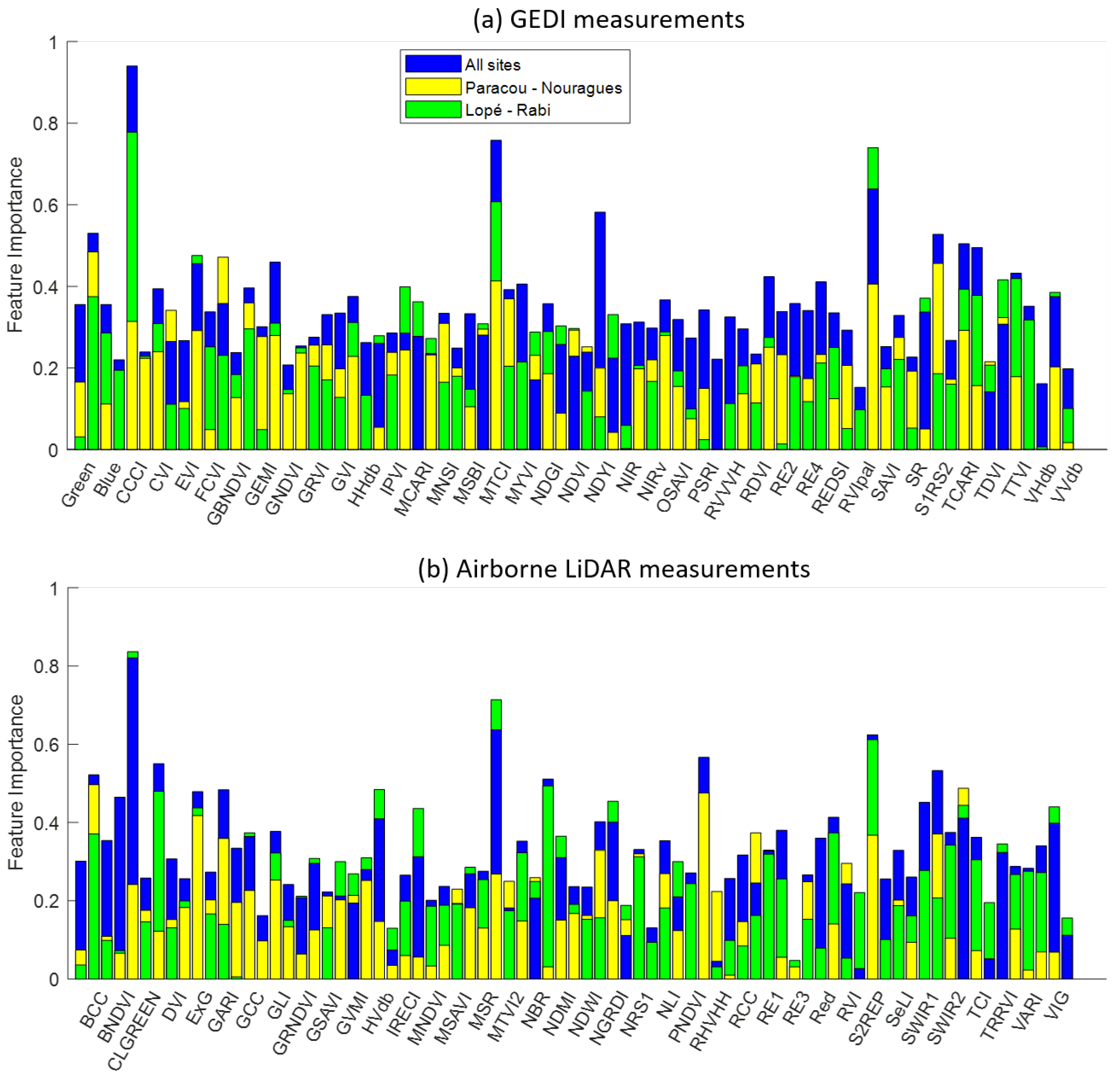
Figure 4.
Proposed feature selection. Feature importance trained from GEDI data in all sites is reported. Stability index in both airborne LiDAR and GEDI: (2) BCC (blue chromatic coordinate), (5) CCCI (canopy chlorophyll content index), (10) ExG (excess green index), (14) GCC (green chromatic coordinate), (16) GLI (green leaf index), (33) MTCI (MERIS terrestrial chlorophyll index), (54) RE1 (red edge 1), (62) S2REP (Sentinel-2 red-edge position), and (69) TCARI (transformed chlorophyll absorption in reflectance index).

Figure 5.
The predicted CHM performance with respect to airborne LiDAR. (a) training by GEDI and total features. (b) training by GEDI and only nine selected features: BCC, CCCI, ExG, GCC, GLI, MTCI, RE1, S2REP and TCARI.
Figure 5.
The predicted CHM performance with respect to airborne LiDAR. (a) training by GEDI and total features. (b) training by GEDI and only nine selected features: BCC, CCCI, ExG, GCC, GLI, MTCI, RE1, S2REP and TCARI.
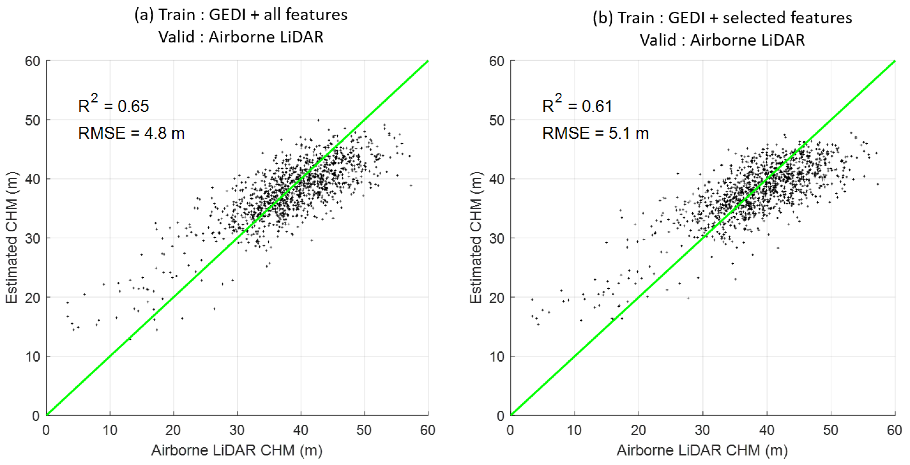
Figure 6.
Feature importance in descending order. (a) Optical selected features: CCCI, MTCI, GCC, BCC, GLI, ExG, TCARI, RE1, S2REP. (b) Radar features: HVdb, VHdb, RVI, HHdb, RVVVH, VVdb, RHVHH, RVIpal.
Figure 6.
Feature importance in descending order. (a) Optical selected features: CCCI, MTCI, GCC, BCC, GLI, ExG, TCARI, RE1, S2REP. (b) Radar features: HVdb, VHdb, RVI, HHdb, RVVVH, VVdb, RHVHH, RVIpal.

Figure 7.
The predicted CHM performance by combining optical and radar-selected features to airborne LiDAR. They include nine Sentinel-2 (BCC, CCCI, ExG, GCC, GLI, MTCI, RE1, S2REP, and TCARI) and HV PALSAR-2 features.
Figure 7.
The predicted CHM performance by combining optical and radar-selected features to airborne LiDAR. They include nine Sentinel-2 (BCC, CCCI, ExG, GCC, GLI, MTCI, RE1, S2REP, and TCARI) and HV PALSAR-2 features.
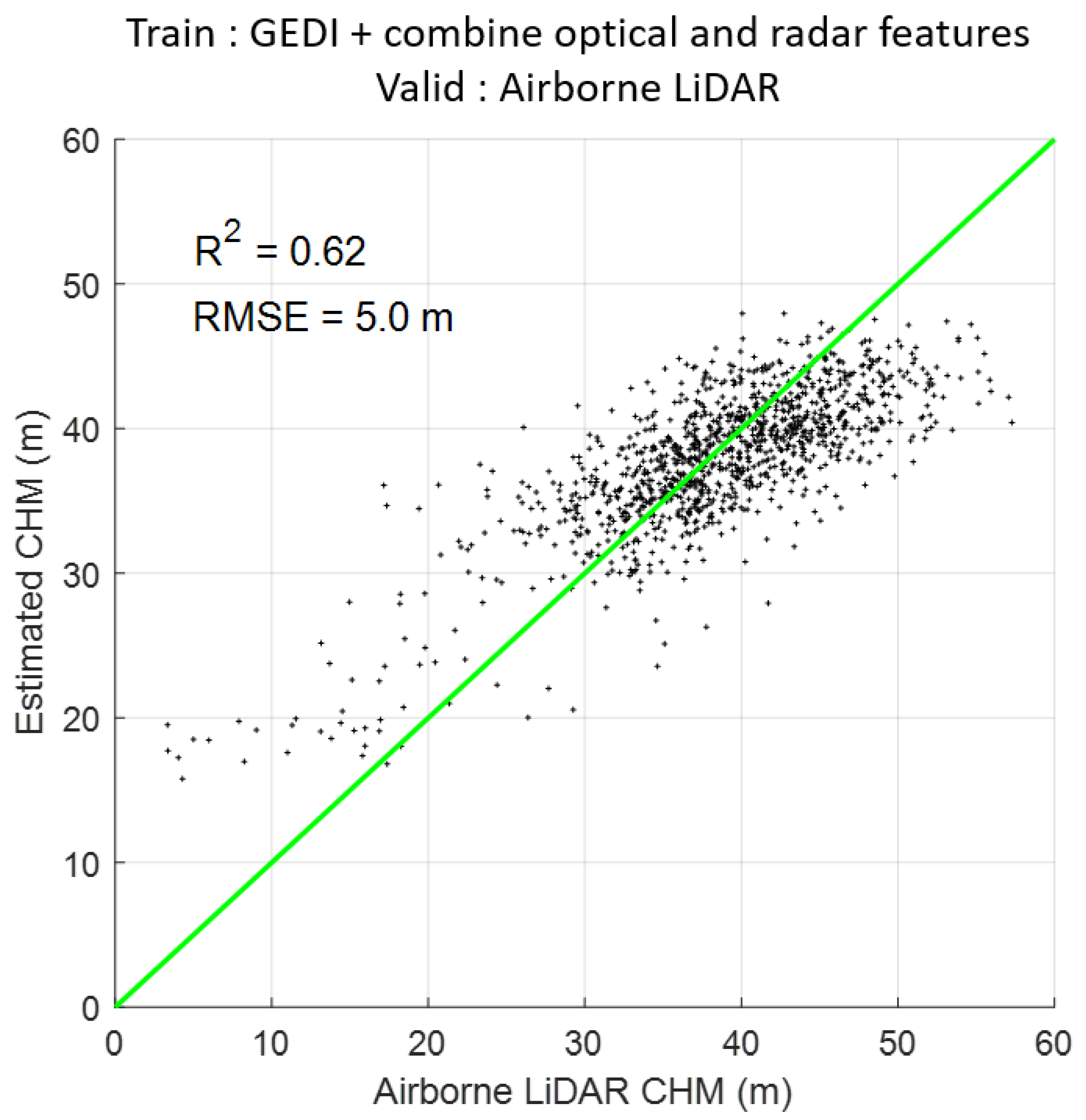
Figure 8.
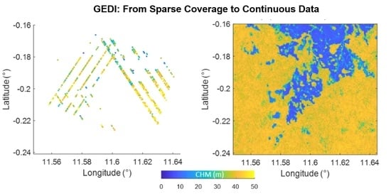
The predicted CHM map compared to the GEDI points in four forest areas. Left panels: sparse GEDI data available after filtering as in Section 2.2. Middle panels: wall-to-wall CHM maps using optical and radar-selected features. Right panels: standard Sentinel-2 red, green, and blue bands of a composite RGB image, in which the green color indicates forest areas. (a): Paracou. (b): Nouragues. (c): Rabi. (d): Lopé.
Figure 8.
The predicted CHM map compared to the GEDI points in four forest areas. Left panels: sparse GEDI data available after filtering as in Section 2.2. Middle panels: wall-to-wall CHM maps using optical and radar-selected features. Right panels: standard Sentinel-2 red, green, and blue bands of a composite RGB image, in which the green color indicates forest areas. (a): Paracou. (b): Nouragues. (c): Rabi. (d): Lopé.
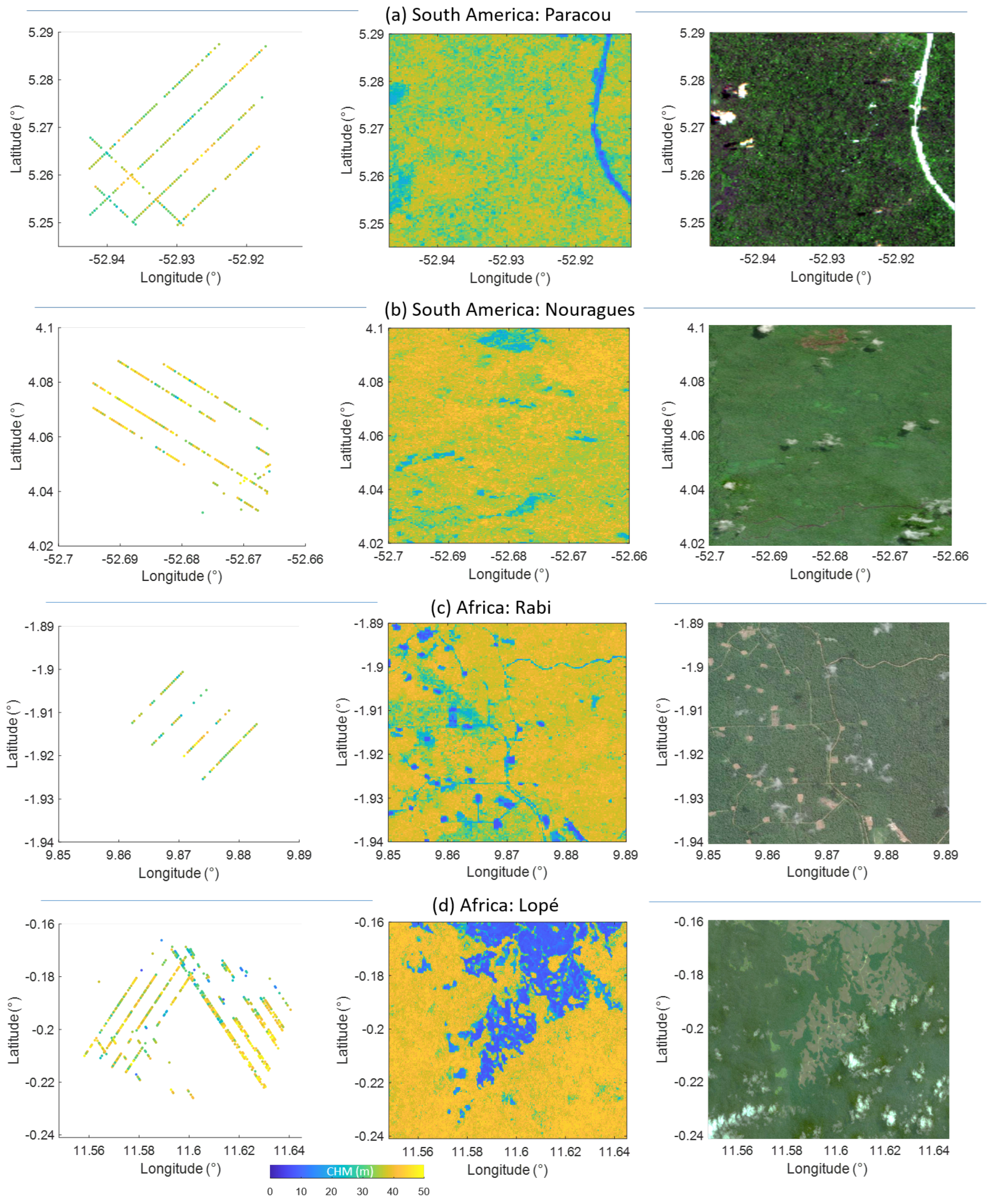
Figure 9.
The predicted CHM compared to the airborne LiDAR validation data in cross-validation between South America and Africa.
Figure 9.
The predicted CHM compared to the airborne LiDAR validation data in cross-validation between South America and Africa.

Figure 10.
The predicted CHM compared to the airborne LiDAR validation data. (a) Validation in Africa (AF). (b) Validation in South America (SA).
Figure 10.
The predicted CHM compared to the airborne LiDAR validation data. (a) Validation in Africa (AF). (b) Validation in South America (SA).


Table 1.
Characteristics of the indicators. The radar index is highlighted in bold font. The symbol used in the expression follows the mapping standard of Sentinel-2: A (Aerosol)—B1; B (Blue)—B2; G (Green)—B3; R (Red)—B4; RE1 (Red Edge 1)—B5; RE2 (Red Edge 2)—B6; RE3 (Red Edge 3)—B7; RE4 (Red Edge 4)—B8A; N (NIR)—B8, S1 (SWIR 1)—B11; S2 (SWIR 2)—B12. g is a gain factor for the enhanced vegetation index (EVI). ‘**’ is the pow operator.
| ID | Indices | Description | Formulation |
|---|---|---|---|
| (1) | Green | Green | G |
| (2) | BCC [26] | Blue Chromatic Coordinate | B/(R + G + B) |
| (3) | Blue | Blue | B |
| (4) | BNDVI [27] | Blue Normalized Difference Vegetation Index | (N − B)/(N + B) |
| (5) | CCCI [28] | Canopy Chlorophyll Content Index | ((N − RE1)/(N + RE1))/(( N − R)/(N + R)) |
| (6) | CLGREEN [29] | Chlorophyll Index Green | (N/G) − 1.0 |
| (7) | CVI [30] | Chlorophyll Vegetation Index | (N/G) × (R/G) |
| (8) | DVI [31] | Difference Vegetation Index | N − R |
| (9) | EVI [32] | Enhanced Vegetation Index | g × (N − R)/(N + C1 × R − C2 × B + L) |
| (10) | ExG [33] | Excess Green Index | 2 × G − (R + B) |
| (11) | FCVI [34] | Fluorescence Correction Vegetation Index | N − ((R + G + B)/3.0) |
| (12) | GARI [35] | Green Atmospherically Resistant Vegetation Index | (N − (G − (B − R)))/(N − (G + (B − R))) |
| (13) | GBNDVI [36] | Green-Blue Normalized Difference Vegetation Index | (N − (G + B))/(N + (G + B)) |
| (14) | GCC [26] | Green Chromatic Coordinate | G/(R + G + B) |
| (15) | GEMI [37] | Global Environment Monitoring Index | ((2.0 × ((N ** 2.0) − (R ** 2.0)) + 1.5 × N + 0.5 × R)/ (N + R + 0.5)) × (1.0 − 0.25 × ((2.0 × ((N ** 2.0) − (R ** 2)) + 1.5 × N + 0.5 × R)/(N + R + 0.5))) − ((R − 0.125)/(1 − R)) |
| (16) | GLI [38] | Green Leaf Index | (2.0 × G − R − B)/(2.0 × G + R + B) |
| (17) | GNDVI [35] | Green Normalized Difference Vegetation Index | (N − G)/(N + G) |
| (18) | GRNDVI [36] | Green-Red Normalized Difference Vegetation Index | (N − (G + R))/(N + (G + R)) |
| (19) | GRVI [39] | Green Ratio Vegetation Index | N/G |
| (20) | GSAVI [40] | Green Soil-Adjusted Vegetation Index | (N − G)/((N + G + 0.5) × (1 + 0.5)) |
| (21) | GVI [40] | Green Vegetation Index | (−0.290 × G − 0.562 × R + 0.600 × RE1 + 0.491 × N) |
| (22) | GVMI [41] | Global Vegetation Moisture Index | ((N + 0.1) − (S2 + 0.02))/((N + 0.1) + (S2 + 0.02)) |
| (23) | lHHdb | PALSAR-2 HH | HH |
| (24) | HVdb | PALSAR-2 HV | HV |
| (25) | IPVI [42] | Infrared Percentage Vegetation Index | ((N/(N + R))/2) × ((N − R)/(N + R) + 1) |
| (26) | IRECI [43] | Inverted Red-Edge Chlorophyll Index | (RE3 − R)/(RE1/RE2) |
| (27) | MCARI [43] | Modified Chlorophyll Absorption in Reflectance Index | ((RE1 − R) − 0.2 × (RE1 − G)) × (RE1/R) |
| (28) | MNDVI [44] | Modified Normalized Difference Vegetation Index | (N − S2)/(N + S2) |
| (29) | MNSI [45] | Misra Non Such Index | −0.404 × G − 0.039 × R − 0.505 × RE1 + 0.762 × N |
| (30) | MSAVI [46] | Modified Soil-Adjusted Vegetation Index | 0.5 × (2.0 × N + 1 − (((2 × N + 1) ** 2) − 8 × (N − R)) ** 0.5) |
| (31) | MSBI [45] | Misra Soil Brightness Index | 0.406 × G + 0.600 × R + 0.645 × RE1 + 0.243 × N |
| (32) | MSR [47] | Modified Simple Ratio | (N/R − 1)/((N/R + 1) ** 0.5) |
| (33) | MTCI [43] | MERIS Terrestrial Chlorophyll Index | (RE2 − RE1)/(RE1 − R) |
| (34) | MTVI2 [48] | Modified Triangular Vegetation Index 2 | (1.5 × (1.2 × (N − G) − 2.5 × (R − G)))/((((2.0 × N + 1) ** 2) − (6.0 × N − 5 × (R ** 0.5)) − 0.5) ** 0.5) |
| (35) | MYVI [45] | Misra Yellow Vegetation Index | −0.723 × G − 0.597 × R + 0.206 × RE1 − 0.278 × N |
| (36) | NBR [49] | Normalized Blue Red | (N − S2)/(N + S2) |
| (37) | NDGI [50] | Normalized Difference Greenness Index | (G − R)/(G + R) |
| (38) | NDMI [49] | Normalized Difference Moisture Index | (N − S1)/(N + S1) |
| (39) | NDVI [42] | Normalized Difference Vegetation Index | (N − R)/(N + R) |
| (40) | NDWI [49] | Normalized Difference Water Index | (N − S2)/(N + S2) |
| (41) | NDYI [51] | Normalized Difference Yellowness Index | (G − B)/(G + B) |
| (42) | NGRDI [52] | Normalized Green Red Difference Index | (G − B)/(G + B) |
| (43) | NIR | NIR | N |
| (44) | NRS1 | NIR/SWIR1 | N/S1 |
| (45) | NIRv [53] | Near-Infrared Reflectance of Vegetation | ((N − R)/(N + R)) × N |
| (46) | NLI [54] | Non-Linear Vegetation Index | ((N ** 2) − R)/((N ** 2) + R) |
| (47) | OSAVI [55] | Optimized Soil-Adjusted Vegetation Index | (1.16) × (N − R)/(N + R + 0.16) |
| (48) | PNDVI [11] | Pan NDVI | (N − (B + G + R))/(N + (B + G + R)) |
| (49) | PSRI [56] | Plant Senescence Reflectance Index | (R − B)/RE2 |
| (50) | RHVHH | PALSAR-2 HV/HH | HV/HH |
| (51) | RVVVH | Sentinel-1 VV/VH | VV/VH |
| (52) | RCC [26] | Red Chromatic Coordinate | R/(R + G + B) |
| (53) | RDVI [57] | Renormalized Difference Vegetation Index | (N − R)/((N + R) ** 0.5) |
| (54) | RE1 | Red Edge 1 | RE1 |
| (55) | RE2 | Red Edge 2 | RE2 |
| (56) | RE3 | Red Edge 3 | RE3 |
| (57) | RE4 | Red Edge 4 | RE4 |
| (58) | Red | Red | R |
| (59) | REDSI [58] | Red-Edge Disease Stress Index | ((705.0 − 665.0) × (RE3 − R) − (783.0 − 665.0) × (RE1 − R))/ (2.0 × R) |
| (60) | RVI [59] | Radar Vegetation Index Sentinel-1 | (4 × VHdb)/(VVdb + VHdb) |
| (61) | RVIpal [59] | Radar Vegetation Index PALSAR-2 | (4 × HVdb)/(HHdb + HVdb) |
| (62) | S2REP [43] | Sentinel-2 Red-Edge Position | 705.0 + 35.0 × ((((RE3 + R)/2.0) − RE1)/(RE2 − RE1)) |
| (63) | SAVI [60] | Soil-Adjusted Vegetation Index | (1.0 + L) × (N − R)/(N + R + L) |
| (64) | SeLI [61] | Sentinel-2 LAI Green Index | (RE4 − RE1)/(RE4 + RE1) |
| (65) | SR [62] | Simple Ratio | N/R |
| (66) | SWIR1 | SWIR1 | S1 |
| (67) | S1RS2 | SWIR1/SWIR2 | S1/S2 |
| (68) | SWIR2 | SWIR2 | S2 |
| (69) | TCARI [63] | Transformed Chlorophyll Absorption in Reflectance Index | 3 × ((RE1 − R) − 0.2 × (RE1 − G) × (RE1/R)) |
| (70) | TCI [64] | Triangular Chlorophyll Index | 1.2 × (RE1 − G) − 1.5 × (R − G) × (RE1/R) ** 0.5 |
| (71) | TDVI [65] | Trasformed NDVI | 1.5 × ((N)/((N ** 2 + R + 0.5) ** 0.5)) |
| (72) | TRRVI [66] | Transformed Red Range Vegetation Index | ((RE2 − R)/(RE2 + R))/(((N − R)/(N + R)) + 1.0) |
| (73) | TTVI [67] | Transformed Triangular Vegetation Index | 0.5 × ((865.0 − 740.0) × (RE3 − RE2) − (RE4 − RE2) × (783.0 − 740)) |
| (74) | VARI [39] | Visible Atmospherically Resistant Index | (RE1 − 1.7 × R + 0.7 × B)/(RE1 + 1.3 × R − 1.3 × B) |
| (75) | VHdb | Sentinel-1 VH | VH |
| (76) | VIG [39] | Vegetation Index Green | (G − R)/(G + R) |
| (77) | VVdb | Sentinel-1 VV | VV |
Disclaimer/Publisher’s Note: The statements, opinions and data contained in all publications are solely those of the individual author(s) and contributor(s) and not of MDPI and/or the editor(s). MDPI and/or the editor(s) disclaim responsibility for any injury to people or property resulting from any ideas, methods, instructions or products referred to in the content. |
© 2023 by the authors. Licensee MDPI, Basel, Switzerland. This article is an open access article distributed under the terms and conditions of the Creative Commons Attribution (CC BY) license (https://creativecommons.org/licenses/by/4.0/).
Share and Cite
MDPI and ACS Style
Ngo, Y.-N.; Ho Tong Minh, D.; Baghdadi, N.; Fayad, I. Tropical Forest Top Height by GEDI: From Sparse Coverage to Continuous Data. Remote Sens. 2023, 15, 975. https://doi.org/10.3390/rs15040975
AMA Style
Ngo Y-N, Ho Tong Minh D, Baghdadi N, Fayad I. Tropical Forest Top Height by GEDI: From Sparse Coverage to Continuous Data. Remote Sensing. 2023; 15(4):975. https://doi.org/10.3390/rs15040975
Chicago/Turabian StyleNgo, Yen-Nhi, Dinh Ho Tong Minh, Nicolas Baghdadi, and Ibrahim Fayad. 2023. "Tropical Forest Top Height by GEDI: From Sparse Coverage to Continuous Data" Remote Sensing 15, no. 4: 975. https://doi.org/10.3390/rs15040975
Note that from the first issue of 2016, this journal uses article numbers instead of page numbers. See further details here.