
A Statistical Study of Ion Upflow during Periods of Dawnside Auroral Polarization Streams and Subauroral Polarization Streams

Department of Space Physics, School of Electronic Information, Wuhan University, Wuhan 430072, China
*
Author to whom correspondence should be addressed.
Remote Sens. 2023, 15(5), 1320; https://doi.org/10.3390/rs15051320
Submission received: 17 January 2023
/
Revised: 22 February 2023
/
Accepted: 23 February 2023
/
Published: 27 February 2023
(This article belongs to the Special Issue Applications of Remote Sensing in Monitoring Ionospheric Physics and Ionospheric Weather Forecasting)
Abstract
:We have investigated the effect of the dawnside subauroral polarization stream (SAPS) and dawnside auroral polarization stream (DAPS) on the ionospheric ion upflow in the Northern Hemisphere by using four years of Defense Meteorological Satellite Program (DMSP) observations. The occurrence rate of DAPS is higher than that of dawnside SAPS. Obvious ion upflow occurs in the topside ionosphere around the DAPS region. The effect of the dawnside SAPS on the vertical flow is weakened when geomagnetic activity increases. There are prominent upflow fluxes around the DAPS, while there are insignificant upflow fluxes around the SAPS region. The plasma density trough during SAPS periods becomes shallower with increasing magnetic activity. These variations with magnetic activity might be due to the weakened ion-neutral collision heating efficiency during highly disturbed periods. There is no obvious plasma density trough or ion temperature drop around the DAPS region at the altitude of ~800 km. The ion temperature around the SAPS area decreases, while the electron temperature increases around the DAPS and SAPS regions.
1. Introduction
The subauroral polarization stream (SAPS) is an interesting and important phenomenon in the subauroral region and is characterized by rapid sunward plasma flow [1]. The SAPS is intrinsically related to the midlatitude trough [2,3], region-2 field-aligned currents (R2 FACs) and the location of the plasmapause. In addition, the SAPS plays a very important role in the injection and energization of plasma in the inner magnetosphere [4,5]. Previous researchers have conducted in-depth studies on the spatial and temporal distributions of duskside SAPS [6]. The SAPS velocity is controlled by the convection electric field and ionospheric conductance, and there is an exponential relationship between the SAPS latitude and the Dst index [7]. With increasing magnetic local time (MLT), the duskside–premidnight SAPS channel narrows and the peak ion flux decreases [8]. The SAPS latitude and velocity exhibit hemispheric asymmetries [9]. There is a good linear relationship between the SAPS magnetic latitude (MLat) and MLT during the quiet period, but this relationship becomes nonlinear with increasing geomagnetic activity [10]. The SAPS can lead to a reduction in the total electron density content in the midlatitude region and reflect the formation of a plasmaspheric plume during magnetic storms, generate large vertical plasma upflows, form an ionization density trough in the F region, drive the westward and meridional wind jets, and have a significant impact on the equatorial electrojet [1,11,12,13,14,15,16,17,18]. Small-scale wave structures of the duskside SAPS were investigated in relation to the plasma and field disturbances [19,20]. In addition, some abnormal SAPS structures have been reported; for example, double-peak subauroral ion drift (DSAID) tends to occur during the geomagnetically active period, which is related to the double-peak structure of R2 FACs, the midlatitude trough ion temperature or the double-trough structure of ionospheric conductivity [21,22]. Sinevich et al. (2022) [23] also confirmed the existence of DSAID by studying the spatial structure of SAID with an extremely high temporal resolution based on data from the NorSat-1 and Swarm-C satellites. They showed that the SAID consists of several strata that include many small-scale irregularities. The anomaly SAPS (ASAPS), the eastward flow in the dusk sector, is related to the overshielding effect in the inner magnetosphere [24].
The ionospheric upflow is essential in the magnetosphere–ionosphere coupling process, which has been investigated by a lot of studies mainly focusing on the polar cusp and auroral regions [25]. Several works have investigated the close relationship between the SAPS and ion upflow in the ionosphere. Using Millstone Hill radar observations, Yeh and Foster (1990) [26] studied ion upflow events during strong magnetic storms. They found that the ion upward velocity increased sharply at heights above 600 km and could exceed 3000 m/s at 1000 km. It was also revealed that energetic particle precipitation and ion heating were the main acceleration mechanisms of oxygen ions (O+). Anderson et al. (1991) [27] observed large upflow ion velocities as a common feature corresponding to the subauroral ion drift (SAID, which has a stronger and narrower sunward flow than the SAPS) events with Atmosphere Explorer C and Dynamics Explorer 2 spacecraft. Heelis et al. (1993) [28] simulated the effect of subauroral ion drift (SAID, which has a stronger and narrower sunward flow than the SAPS) on the ionosphere below 1500 km and found that the friction heating of the F layer led to the upward movement of ions, while the reduction in plasma density further enhanced SAID. Erickson et al. (2010) [29] observed that the upward ion flux caused by the SAPS during storms could reach 5 × 109 cm−2s−1, related to the increased ion temperature [30]. Wang and Lühr (2013) [31] conducted a statistical study on the seasonal variation in ion upflow caused by the SAPS and found that the ion upward flow velocity had a good correlation with the SAPS velocity. The peak of the average ion upward flow was highest in winter, reaching 2 × 108 cm−2s−1, which is comparable to the upward flux in the typical upward flow region around the polar cusp [32]. Khalipov et al. (2016) [33] analyzed the results of measurements of vertical and horizontal motions of plasma by comparing Doppler data from ground-based ionosondes and driftometer data from DMSP satellites and found constant upflow over SAID bands under the assumption that the SAID is embedded in the SAPS structure. By using vertical radio sounding and Doppler measurements at the subauroral ionospheric station, Stepanov et al. (2019) [34] revealed that the times and locations of peaks of the vertical and horizontal plasma drift velocity may not coincide, which is because the vertical velocities may differ in time and direction during the development of SAID. Zhang et al. (2020) [35] found that upward flows could usually be observed near the SAPS region, and the temporal and spatial distributions of the occurrence rate and velocity of the SAPS during different substorm intensities were consistent with those of upward ion events. They showed that there was a moderate linear relationship between the ion upward flow and SAPS velocity. The above research work showed that the duskside ionosphere at midlatitudes is an important source region of magnetospheric O+, and the frictional heating caused by the SAPS may be one of the important physical factors driving the upward flow.
Similar to the duskside SAPS, fast eastward plasma flow occurs in the dawnside subauroral region, which is called the dawnside SAPS [36,37]. However, it is not known whether the dawnside SAPS is also the important source of ion upflow. To the best of our knowledge, most SAPS studies have focused on the dusk-midnight sector, while there is no clear understanding of the spatial distribution or effect of the SAPS of the dawn convection cell. Lin et al. (2022) [38] used Defense Meteorological Satellite Program (DMSP) satellite observations and Multiscale Atmosphere Geospace Environment (MAGE) model simulations to study the possible generation mechanism of the dawnside SAPS for the first time. They revealed that the morning SAPS occurred only under very strong magnetic storms. This was because the magnetospheric plasma convection during enhanced activities was sufficiently strengthened to transport energetic ions to the morning sector. The accumulation of ions could enhance the pressure gradient of the ring current, thus generating strong R2 FACs in the subauroral region to finally drive the SAPS. However, statistical studies on the relationship between the dawnside SAPS and ion upflow are still lacking. Whether the dawnside subauroral region is also an important source region for inner magnetospheric O+ ions remains unknown and needs further study.
The SAPS occurs equatorward of the auroral oval, while on the poleward side of aurora oval, the dawnside auroral polarization stream (DAPS) flows in the eastward direction. Using DMSP and Swarm satellite observations, Liu et al. (2020) [39] revealed that the DAPS occurred around the boundary of R1 and R2 FACs in the dawn sector, which was related to the significant equatorward gradient of conductivity at the boundary. When the geomagnetic activity increased, the whole auroral-zone conductance increased; thus, the conductivity difference at the boundary of the R1 and R2 FACs became negligible. As a consequence, the DAPS could be suppressed. They believed that enhanced R2 FACs favor DAPS occurrence. Interestingly, Liu et al. (2020) [39] reported that during a DAPS event, obvious upward ion flow could be observed around the DAPS. This indicated that the DAPS could cause the upflow of ionospheric ions. However, these findings were based on case studies and have not been statistically verified. No comparison between DAPS and SAPS effects has yet been reported.
This paper uses the plasma observations of the DMSP F16 satellite from 2015 to 2018 to carry out a statistical study on the ion upward flow caused by the SAPS and DAPS in the dawn sector, focusing on their responses to geomagnetic activities. A comparative analysis of their effects on the ionosphere is further explored. The O+ ions from dawnside SAPS or the DAPS region can be energized due to several possible causes [31,40]. For SAPS, ion friction heating is regarded as an important mechanism for the upward flow of ions in the subauroral region. For DAPS, the soft electrons that precipitate into the high-latitude ionosphere may modulate the electron pressure gradient to form the bipolar electric field to accelerate ion upflow. In addition, the plasmasphere could conduct heat down to the top ionosphere through the interaction between plasmaspheric waves and ionospheric electrons. This study will be of great significance in understanding the transport paths of ionospheric particles and the amount of O+ ions possibly sourced to the magnetospheric ring current. It should be noted that the ion upflows in the top ionosphere are studied in the present work. O+ ions need to be further energized so as to outflow to the ring current region.
2. Dataset and Method of Statistical Analysis
The DMSP F16 satellite is flying at an altitude of approximately 850 km with an approximately 100 min orbital period. The sun-synchronous orbits are approximately 0400–1600 in the MLT sector. The ion drift meter (IDM) onboard F16 can measure ion drift velocities in both the cross-track and vertical directions. Both dawnside SAPS and DAPS events are identified from cross-track velocities, while ion upflow events are detected from vertical velocities. To guarantee that the DMSP cross-track direction is approximately aligned with the auroral oval, the orbits with angles less than 45° between the auroral ovals have been discarded. F16 is equipped with a scintillation meter, retarding potential analyzer, and Langmuir probe; these instruments can measure the ion density, ion temperature and electron temperature, respectively.
By using the DMSP spectrometer (SSJ/4), the average energy flux of precipitating electrons and ions is monitored in the range of 30 eV to 30 keV, from which the height-integrated ionospheric conductivity can be derived [41,42]. The peak auroral conductance can be determined along the satellite orbit. Then, we step equatorward until the conductance is reduced to 0.2 times the peak value or to 1 S, whichever is smaller. This can be identified as the equatorward boundary of the auroral oval. In the subauroral region, a peak eastward drift greater than 500 m/s is identified as a dawnside SAPS event. More details about the SAPS selection method in the dusk sector can be found in Wang et al. (2008) [7]. Figure 1a shows one example of a SAPS at 4.81 MLT at approximately 18.03 UT on 18 March 2015. From top to bottom in the left column, Figure 1a provides ionospheric Pedersen conductance due to particle precipitation, cross-track plasma velocity, and vertical velocity information. The right column of Figure 1a shows the zonal component of the ionospheric magnetic field with Earth’s main field subtracted (positive denotes the eastward direction), and the differential energy flux of ion and electron precipitations. The magnetic field intensifies in the westward direction with increasing latitude from 54° to 67° MLat, which is upward R2 FACs. The magnetic field recovers towards the eastward direction after 67° MLat, which is downward of R1 FACs. Enhanced ion and electron precipitations can be found in the auroral region. SAPS (positive denotes the eastward direction) is located in the subauroral region with less electron and ion precipitations, and in the equatorward region of R2 FACs. The peak velocity of the SAPS is indicated by the vertical dashed line. Collocated with the SAPS, there is an enhanced upward velocity (positive denotes the upward direction).
The DAPS is mainly caused by the steep equatorward conductance gradient in the poleward side of the auroral oval [39]. By using the Swarm electric and magnetic field measurements, Olifer et al. (2021) [43] revealed that the ionospheric conductance was obviously larger in the upward R2 FACs than in the downward R1 FACs on the dawnside due to energetic electron precipitation in the upward FACs region. Olifer et al. (2021) [43] explained that the precipitation electrons with energy levels of 1–10 keV in the dawn sector were associated with the electron injections from the magnetotail, which tended to deflect toward dawn due to the magnetic field gradient and curvature drift. Therefore, starting from the peak conductance in the auroral oval, we move poleward until the conductance decreases to 0.3 times the peak value. If the conductance decreases by more than 50% within 0.5° MLat, the point can be positioned as the auroral oval with a sharp conductance gradient in the poleward side. A DAPS event can be identified if the peak eastward velocity within ±1° MLat around the relevant boundary exceeds 500 m/s. The DAPS events in Liu et al. (2020) [39] can be selected automatically by this method. Figure 1b shows one example of DAPS at 5.36 MLT at approximately 11.96 UT on 4 January 2015. Similar to Figure 1a,b provides the ionospheric Pedersen conductance due to particle precipitation, zonal velocity, and vertical velocity in the left column. In the right column, we show the eastward component of the magnetic field (positive denotes the eastward direction) and the differential energy flux of ion and electron precipitations. The magnetic field shows a westward increase with increasing latitude until 67° MLat, which corresponds to upward R2 FACs. Poleward of 67° MLat, the magnetic field recovers to the eastward direction with increasing latitude, which is downward R1 FAC. The upward R2 FACs correspond to more intense ion and electron precipitations and inverted-V electron precipitation, when compared to downward R1 FACs. The peak eastward velocity, reaching more than 3000 m/s, as indicated by the vertical dashed line, can be found near the poleward boundary of R2 FACs, which satisfies the definition of DAPS. Collocated with the DAPS, enhanced upward velocity can also be noticed (positive denotes the upward direction).
Four years of DMSP observations (2015–2018) in the Northern Hemisphere during 2015–2018 were processed, and 3526 DAPS and 444 dawnside SAPS events were selected as a result. Four seasons under two different geomagnetic conditions were separately divided to better analyze the seasonal and geomagnetic activity variations. Each season covers three months; the June solstice (JuneS) covers the period from June to August, the December solstice (DeceS) covers December, January, and February, and the remaining six months are related to the March and September equinoxes (MarcE and SeptE). The Kp indices were checked to distinguish whether an event occurred in a disturbed (Kp ≥ 3) or less-disturbed (Kp < 3) period. In this way, the number of events in each season and Kp condition were obtained, and they are listed in Table 1. The occurrence frequency was obtained by dividing the event number by the satellite orbit number in each bin, as shown in the brackets in Table 1. In general, the SAPS occurrence frequency was below 5% when Kp < 3 and less than 16% when Kp ≥ 3. There were fewer SAPS events in the June solstice than in the other seasons. The SAPS occurrence frequency was somewhat lower than that of DAPS, and the latter was approximately 30% when Kp < 3 and approximately 50% when Kp ≥ 3. Thus, the DAPS was detected more frequently than the SAPS on the dawnside. With increasing geomagnetic activity, the occurrence frequencies of both the DAPS and SAPS increased in all seasons.
3. Statistical Results
Figure 2 shows the DAPS and dawnside SAPS event numbers as a function of the MLat. The DAPS events were located mostly at approximately 71° MLat and 69° MLat in the less-disturbed and more-disturbed periods, respectively. The dawnside SAPS were centered at approximately 64° MLat and 56° MLat when AE < 200 and AE ≥ 200, respectively. The DAPS events were located poleward of the dawnside SAPS events. This was because DAPS events occurred around the poleward boundary of the bright aurora, while SAPS events occurred equatorward of the auroral oval. Both DAPS and SAPS events shifted equatorward with the aurora when the magnetic activity increased. It can be seen that SAPS changes significantly with AE, while DAPS changes relatively weakly. This difference might be related to the different locations of DAPS and SAPS relative to the auroral oval. DAPS is located near the boundary between R1 and R2 FACs, so it is closer to the poleward boundary of the auroral oval. SAPS is located equatorward of the auroral oval, and closer to the equatorward boundary of the auroral oval. The equatorward boundary of aurora oval moves more drastically towards low latitude with increasing magnetic activity, compared with the poleward boundary [44]. As a result, the auroral oval region widens in latitudinal span with the increase of magnetic activity. This might explain the more significant change of SAPS than DAPS due to the enhancement of geomagnetic activity.
Regarding the geographical longitude distribution, both the DAPS and dawnside SAPS events were located within the longitudinal ranges of 120°E~180°E (eastern Asian sector) and −180°W~−30°W (North American sector). Notably, this is not shown in Figure 2 because it does not reflect the real distribution of the SAPS and DAPS. The longitude confinement is caused by the orbital angle selection criteria, i.e., the angle between the orbit track and the auroral oval larger than 45°. These criteria may suppress observations at other longitudes.
To further investigate the latitudinal relation between the ion upflow associated with the DAPS and dawnside SAPS, we performed a superposed epoch analysis. The latitudinal profile of the DMSP data is stacked around the location of the peak DAPS or SAPS, which is taken as the key latitude. A latitudinal range from 20° equatorward to 20° poleward of the key latitude is considered. The mean profiles are obtained with a 2° MLat resolution. Due to the fewer SAPS events compared to DAPS events, we studied the Kp dependence of SAPS without any seasonal separation.
Figure 3 shows the average distributions of the cross-track plasma velocity (Vy) under less-disturbed (Kp < 3) and enhanced geomagnetic activity (Kp ≥ 3). The potential offsets at low latitudes have been removed by using the same method as Hairston et al. (1998) [45] before averaging. We have established a linear baseline for the polar pass by using velocity data around 40° MLat. When the linear baseline (residual velocity) is removed, the velocity at the endpoints (around 40° MLat) can reach zero. Here, we chose the DAPS at MarcE as an example; other seasons showed similar variations and are thus not shown. Figure 3a,b shows the results for DAPS, and Figure 3c,d shows the results for SAPS without seasonal separation. There is a peak eastward flow velocity at the zero latitude, which is a typical feature of DAPS and SAPS eastward flow. In Figure 3c,d, another peak eastward flow occurs in the aurora oval region. The mean peak zonal velocities at the key latitudes are listed in Table 2. When comparing the DAPS and SAPS zonal velocities, it can be seen that those of DAPS are larger than those of SAPS, irrespective of the season or geomagnetic activity level.
Figure 4 shows the latitudinal variation in the ion upflow (Vz) in the same format as Figure 3. The peak upflow velocities are listed in Table 3. For DAPS, there is a clear pattern of enhanced upward flow around the DAPS, indicative of the important effect of the DAPS on the ion upflow. The peak upflow velocities tend to increase with increasing magnetic activity, with the weakest velocities observed at JuneS and MarcE. These variations are generally consistent with those of the DAPS velocities, indicating the close relationship between the DAPS and upflow velocities. The maximum upflow velocity associated with the DAPS reaches 273 m/s at SeptE and increases to 384 m/s as the geomagnetic activity increases.
The dawnside SAPS exhibits different characteristics. During less-disturbed periods (Kp < 3), a peak vertical flow of approximately 167 m/s is observed around the SAPS key latitude. However, during enhanced geomagnetic activity, a weak peak velocity of approximately 116 m/s can be found around the key latitude. At both magnetic levels, another peak vertical velocity occurs poleward of the key latitude, indicating the important upflow in the auroral oval. This indicates that the upflow is less efficiently induced by the SAPS under more-disturbed periods than under less-disturbed periods.
The latitudinal variations in the plasma density at an altitude of approximately 800 km during the DAPS and dawnside SAPS periods are shown in Figure 5. A large plasma density drop occurs equatorward of the DAPS, while the DAPS has a negligible effect on electron density reduction in the higher F region around the key latitude. For the dawnside SAPS, a reduction in the plasma density can be clearly seen around the key latitude for all magnetic activity levels. The peak plasma densities at the key latitude are listed in Table 4; the largest is found at JuneS for the DAPS. The trough density tends to increase with increasing geomagnetic activity for both the DAPS and SAPS, except in the JuneS period.
4. Discussion
4.1. Occurrence Rate
The dawnside SAPS has a lower occurrence rate than the DAPS: below 5% for Kp < 3 and below 16% for Kp ≥ 3. We selected the duskside SAPS as observed by F16 from 2015 to 2018 in a similar way to the dawnside SAPS. The occurrence frequencies of the duskside SAPS are approximately 21% during Kp < 3 and 62.6% during Kp ≥ 3; these values are larger by factors of 3–4 than those of the dawnside SAPS under similar geomagnetic activity levels. Wang and Lühr (2013) [31] investigated the occurrence rate of the duskside SAPS around the 18 MLT sector, as detected by DMSP F13. They reported that the occurrence frequencies of the duskside SAPS were 14% (41%), 11% (28%), 15% (20%), and 11% (28%) at MarcE and SeptE, JuneS and DeceS when Kp < 4 (Kp ≥ 4). The enhanced occurrence rate with geomagnetic activity is consistent with the present work. Lin et al. (2022) [38] investigated the generation mechanism of the dawnside SAPS by using global geospace simulations. They demonstrated that the dawnside SAPS could occur only during very strong activity periods (when Kp is nearly 9) when the electric-field eastward drift was stronger than the magnetic-field westward drift. If the external driving in the model was lowered, the magnetic-field westward drift dominated, and the dawnside SAPS could not occur. The strong magnetospheric plasma convection could effectively transport ring current ions to the dawnside to enhance R2 FACs. When the boundary of the FACs was equatorward of the aurora boundary, the eastward SAPS could develop. During relatively weak magnetic activity, R2 FACs were not strong enough to drive any noticeable dawnside SAPS. The statistical analysis of the relative location of R2 FACs and SAPS region will be left for future work. Figure 6a shows the numbers of SAPS and DAPS events as a function of Kp. The DMSP orbit numbers (divided by four for better visualization) are shown together as bars in the dawn and dusk sectors and are quite small when Kp > 5. The event number of the duskside SAPS (blue curve) tends to peak at a lower magnetic activity than the dawnside SAPS (red curve). Figure 6b shows the occurrence rates of SAPS and DAPS events. Here, the occurrence rate is the event number divided by the satellite orbit number. Due to the few orbit numbers occurring when Kp > 5, the occurrence rate under this condition is not shown. The occurrence rate of duskside SAPS (blue curve) tends to occur over a much broader range of geomagnetic activity levels, whereas the dawnside SAPS (red curve) shows a more significant preference for much stronger geomagnetic activity conditions. Thus, it might be concluded that the strong convection that is necessary for the generation of the dawnside SAPS did not occur very frequently from 2015 to 2018, which might account for the low occurrence of SAPS events in the dawn sector in this period. Figure 6a shows that the DAPS occurrence rate (black curve) is comparable to that of the duskside SAPS (blue curve) under both Kp < 3 and Kp ≥ 3 conditions. The DAPS occurrence rate also shows a high magnetic activity preference, similar to that of SAPS (Figure 6b). Liu et al. (2020) [39] investigated several DAPS cases under different geomagnetic activity levels. They found that the DAPS was caused by enhanced R2 FACs (see also Liu et al. (2021) [46]). This might explain the fact that the DAPS was found to occur more frequently during more active periods in the present work.
4.2. Upward Flow
As seen in Table 2, the peak DAPS velocities around the key latitude are faster at DeceS than at JuneS regardless of magnetic activities. This finding is in line with the duskside SAPS [31], which is inversely proportional to the ionospheric conductivity mainly caused by solar illumination being larger in summer than in winter [47]. The DAPS velocities are enhanced when geomagnetic activities increase as a consequence of intensified R2 FACs during more-disturbed periods. When the stronger R2 FAC flows through the low-conductivity area, a larger electric field is required to form a closed current circuit with the high-latitude R1 FACs. The ion upflow velocity also shows a larger velocity at DeceS than at JuneS and is enhanced with increasing magnetic activities. The similar seasonal and geomagnetic activity variations indicate the important effect of DAPS on the ion upflow. We have performed a correlation study of the DAPS velocity and the SAPS velocity with upflow velocity, which is shown in Figure 7. It can be seen that the correlation coefficients of DAPS are generally good: 0.5 for Kp < 3 and 0.6 for Kp ≥ 3, which further confirms the important effect of DAPS on ion upflow. As can be seen from Figure 7b, the correlation between SAPS and ion upflow is poor for both Kp < 3 and Kp ≥ 3, indicating their weak impact on ion upflow.
Figure 8a,b shows the latitudinal variations in the ion upflow flux in each season for two Kp condition ranges during DAPS periods. The upflow fluxes around the key latitude are listed in Table 5. For the DAPS, overall upward flow can be seen in all seasons and is highest at JuneS and lowest at DeceS due to the larger Ne at JuneS than at DeceS. This tendency is similar under both the Kp < 3 and Kp ≥ 3 situations. The ion upflow flux is larger at MarcE and JuneS than at SeptE and DeceS. The upflow flux during disturbed periods can reach a peak value of 5.3 × 108 cm−2s−1 at JuneS.
In the dusk sector, the peak mean upflow flux during SAPS periods can reach approximately 4.85 × 108 cm−2s−1 for Kp ≥ 3 (figure not shown). The upflow flux value is comparable to the normal range of vertical O+ fluxes in the dusk sector (62–78° MLat) [32]. In the cusp region, the typical upflow fluxes are approximately 2 × 108 cm−2s−1 at quiet times and 5 × 108 cm−2s−1 at active times. Thus, these upflow fluxes are quite comparable to those in the dayside cusp region. This indicates that both the dusk subauroral region and the dawn poleward side of the auroral oval are important sources of ion upflows.
In contrast to the prominent ion upflow around the duskside SAPS, no significant ion upflow flux is observed around the dawnside SAPS. This could be a consequence of the relatively deep density trough and weak upward velocity around the key latitude of the SAPS. The dawnside SAPS is larger during more-disturbed periods, while the upward velocity is weaker during more-disturbed periods. In the subauroral region, the important factor affecting the upflow velocity is the frictional heating caused by ion-neutral collisions. This occurs more effectively and faster in the E and low-F regions [28]. The resulting pressure gradient can cause plasma expansion and upflow. The frictional heating is proportional to the velocity difference of ions and neutrals. Lühr et al. (2007) [48] constructed a high-latitude thermospheric wind pattern from cross-track accelerometer measurements of CHAMP for 131 days, centered on June 2003. They found that the average pattern of thermospheric wind showed an obvious anti-sunward flow over the polar cap and an anticyclonic vortex in the dusk sector. Huang et al. (2017) [49] investigated the relationship between the thermospheric neutral wind and auroral Hall current. They disclosed that in the dusk sector, the zonal wind and equivalent current formed a similar vertical flow pattern under different activity-level conditions. However, on the dawnside, plasma drifts seemed to play a less efficient role for the neutral wind, owing to the Coriolis and centrifugal forces. As shown in Figure 2 of Huang et al. (2017) [49], the neutral winds showed a large equatorward wind at approximately 04 MLT, which increased greatly with geomagnetic activity due to enhanced Joule heating in the auroral region. If the SAPS does not increase to the same extent as the neutral wind when the geomagnetic activity increases, the velocity differences between the ion and neutrals can decrease under more-disturbed periods. As seen from Table 2, there is a small increase in SAPS under more-disturbed periods. Subsequently, the reduced Joule heating might result in reduced upward flow under more-disturbed periods (Table 3). Liu et al. (2022) [50] conducted a statistical analysis of the environmental conditions of ionospheric oxygen outflows on the duskside and found that most outflow events were observed during non-storm times.
4.3. Plasma Density
As seen in Figure 5, there is an obvious plasma density trough collocated with the dawnside SAPS. Ion-neutral frictional heating can convert a large amount of O+ in the top ionosphere to NO+ during SAPS periods. The faster recombination of NO+ with electrons than O+ yields the depletion of plasma density. In addition, the large eastward and upward movement could further deepen the midlatitude trough. As shown in Figure 5, with increasing magnetic activity, the depth of the density trough decreases. This is different from the effect of the duskside SAPS, during which the trough deepens with increasing magnetic activity [31]. As discussed in Section 4.1, during more highly disturbed periods, the friction heating centered around the dawnside SAPS may weaken, and the upward motion will decrease; this may be the reason for the reduced trough depth.
For the DAPS, there is no obvious reduction in the plasma density around the key latitude. The DAPS is located at the poleward side of the bright aurora with a large equatorward conductance gradient. The upward R2 FACs are fed by horizontal currents carried by ions from the downward R1 FACs. In addition, the DAPS could be partly collocated with the R1 current. Although the R1 current is mainly carried by upward electrons, some of it is carried by precipitating ions (see Figures 2g and 3f of Liu et al. 2020 [39]). These precipitating ions may contribute to some plasma density. These processes counteract the decrease in ion density caused by frictional heating, as well as the eastward and vertical transport of ions. All these combined physical processes might explain the negligible change in plasma density around the key latitude of the DAPS at ~800 km altitude. At lower altitudes (i.e., the lower F region and the E region), where most of the Joule heating and thus recombination occurs, DAPS has been observed to be associated with a drop of plasma density [39,51]. Future combined modeling of these processes will likely be necessary to address the plasma density variations related to DAPS more clearly.
4.4. Plasma Temperature
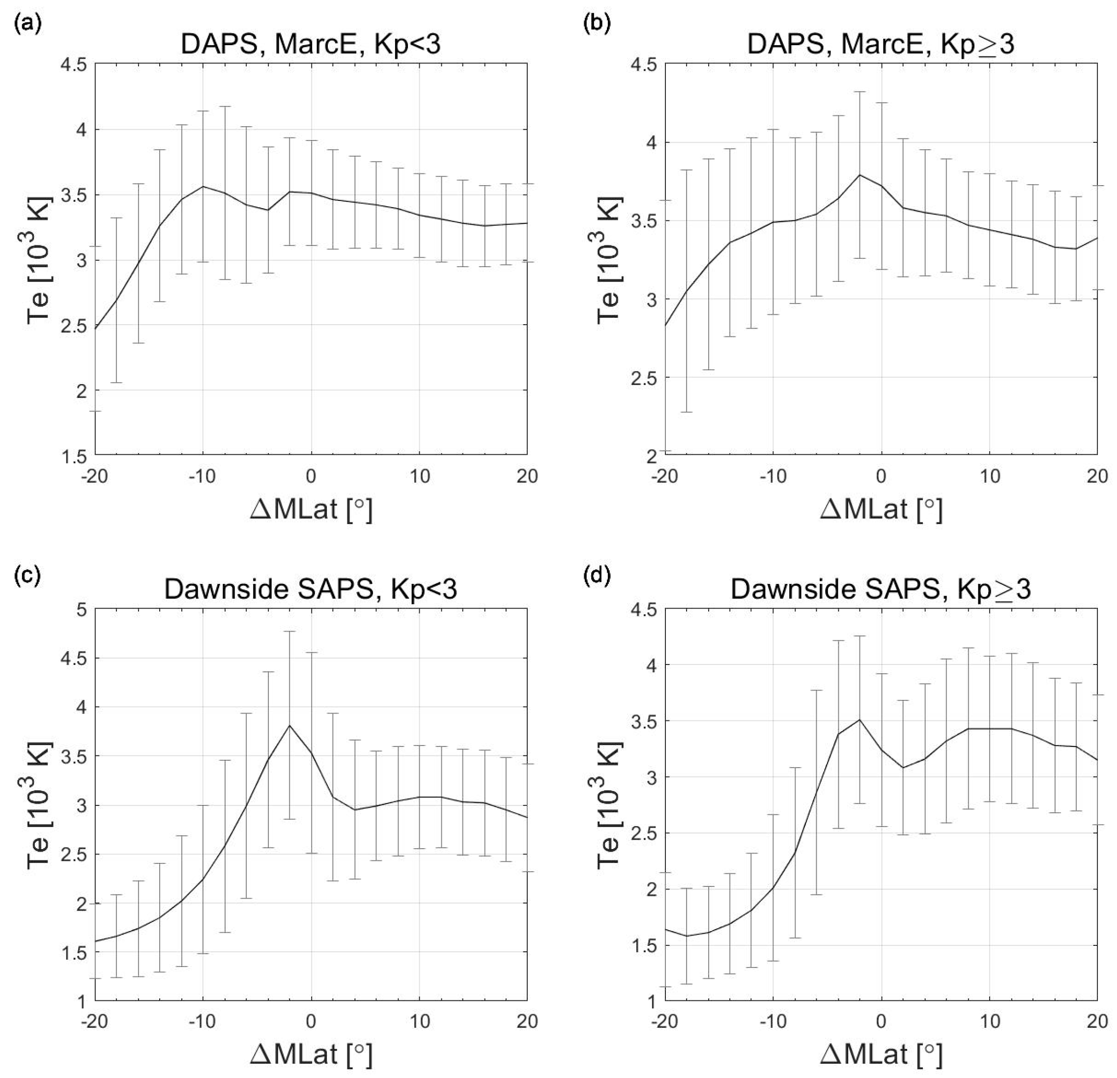
The collision between ion and neutral flows can heat ions efficiently. In Figure 9a,b, the ion temperature during DAPS periods is shown. The DAPS seems to be identified during the poleward gradient of ion temperature. Around the key latitude, no obvious peak or trough of ion temperature can be found in relation to the DAPS. The nonsignificant change in ion temperature is likely related to the altitude of the DMSP observation (approximately 800 km), which is far above where the ion heating processes occur in the E and lower F regions. In addition, as the heated plasma expands from a lower altitude to the DMSP altitude, the adiabatic cooling process plays a leading role. The changes in ion temperature and plasma density are consistent, and both exhibit weak variations (Figure 4). In contrast, the electron temperature around the DAPS region shows enhancement (Figure 10a,b). The electrons might be heated through the deposition of soft electrons into the high-latitude ionosphere. This could modulate the electron pressure gradient in the ionosphere, forming a bipolar electric field to accelerate upward ion movement. Thus, during DAPS periods, both ion and electron heating might play roles in driving the upward flow, which needs to be verified by future model work.
Ion friction heating is regarded as an important mechanism for the upward flow of ions in the subauroral region [31]. Due to ion-neutral friction heating, the ion temperature increases, eventually leading to the upward movement of ions that might enter the inner magnetosphere along the magnetic field line. The ion and electron temperatures at an 800 km altitude during SAPS periods are shown in Figure 9c,d and Figure 10c,d. For SAPS events, one can notice that the ion (electron) temperature has a larger reduction (enhancement) during less-disturbed periods than during more-disturbed periods. Ion temperatures at mid-high latitudes are primarily controlled by ion friction heating from plasma convection and neutrals. The SAPS could induce strong ion friction and reach a peak near the E region. However, the ion temperature around the SAPS region decreases. This indicates that the largely elevated ion temperature due to the friction heating effect is mainly limited to a lower altitude. The reduced ion temperature at the 800 km altitude might be related to the adiabatic cooling process, in which the temperature of ions is proportional to the ion density. When heated ions expand into low-density areas at higher altitudes, the temperature can cool and thus show a lower temperature than the surroundings, which are not involved in the process at the same altitude. With the increase in the geomagnetic activity level, the frictional heating process related to the SAPS tends to weaken, as discussed in Section 4.1; thus, the ion temperature does not further decrease.
In the midlatitude regions, the heating of electrons comes mainly from solar photoelectron heating and heat transport from the plasmasphere, and the cooling of electrons occurs through energy losses to ions and neutrals [52]. Thus, potential processes for the enhanced electron temperature might be Coulomb collisions with ring current energetic ions or to the wave resonant interaction in the plasmasphere/ring current overlap region. The suprathermal electrons in the plasmasphere could conduct heat to the top ionosphere, and subsequently, the electron temperature might be elevated [20]. Another possibility is that due to the decreased plasma density in the SAPS region, the Coulomb collision process between electrons and ions decreases, which could lead to an increase in the electron temperature due to the reduced cooling process. The nearly anti-variations in plasma density and electron temperature around the SAPS region seem to support this conclusion. In fact, Prölss (2006) [53] reported a nearly linear relationship between the observed depletion in electron densities and the enhancement in electron temperatures.
5. Conclusions
In this work, we studied the DAPS and SAPS variations on the dawnside under different magnetic activity conditions, as well as their effects on the ion upflow in the topside ionosphere of the Northern Hemisphere, by using DMSP F16 satellite observations from 2015 to 2018. The main findings are summarized as follows:
- The occurrence rate of the dawnside SAPS is lower than those of both the DAPS and the duskside SAPS. Both the DAPS and SAPS show higher occurrence frequencies under increasing magnetic activity.
- The DAPS velocity is larger than the dawnside SAPS velocity at similar magnetic activity levels. Both zonal velocities are enhanced with increasing magnetic activities. There is a larger DAPS velocity in winter than in summer, similar to the duskside SAPS, which might be due to the relatively low solar illumination in winter.
- The ion upward flow peak around the DAPS shows similar seasonal and magnetic activity variations, indicating a close relationship with the DAPS. A large ion upflow flux can be found around the DAPS region, reaching 5.3 × 108 cm−2s−1 in the June solstice during highly disturbed periods.
- The peak upflow velocity around the dawnside SAPS weakens as the magnetic activity increases, indicating weaker ion-neutral collision heating under more-disturbed periods. There is no obviously enhanced ion upflow flux related to the dawnside SAPS due to the relatively deep midlatitude trough and weak upward velocity.
- The dawnside midlatitude trough is collocated with the SAPS, but its depth becomes shallower with increasing magnetic activity; this is in contrast to the SAPS effect on the duskside. There is a lack of any ion density peak or trough around the DAPS region at the DMSP altitude of ~800 km.
- Around the SAPS region, the ion temperature decreases due to adiabatic cooling in the upper ionosphere, while there is a negligible change around the DAPS region. For both the DAPS and SAPS, the elevated electron temperatures might be explained by heat conduction or Coulomb collisions.
Author Contributions
Conceptualization, C.Q. and H.W.; Methodology, C.Q. and H.W.; Software, C.Q.; Validation, C.Q.; Formal analysis, C.Q. and H.W.; Investigation, C.Q.; Resources, H.W.; Data curation, C.Q.; Writing—original draft, C.Q.; Writing—review & editing, H.W.; Visualization, C.Q.; Supervision, H.W.; Project administration, H.W.; Funding acquisition, H.W. All authors have read and agreed to the published version of the manuscript.
Funding
This research was funded by National Nature Science Foundation of China (41974182), National Natural Science Foundation of China Basic Science Center (42188101), National key research and development program (2022YFF0503700).
Data Availability Statement
The DMSP IDM plasma data and the DMSP SSJ/4 data can be accessible at https://cedar.openmadrigal.org/ accessed on 10 December 2022. The geomagnetic indices data can be downloaded from the website https://omniweb.gsfc.nasa.gov/ accessed on 10 December 2022.
Acknowledgments
We thank the Center for Space Sciences at the University of Texas at Dallas and the US Air Force for providing the DMSP IDM plasma data and the Space Physics Interactive Data Resource (SPIDR) for providing the DMSP SSJ/4 data. The WDC C2 for Geomagnetism at Kyoto are greatly acknowledged for providing the geomagnetic indices data.
Conflicts of Interest
The authors declare no conflict of interest.
References
- Foster, J.C.; Vo, H.B. Average characteristics and activity dependence of the subauroral polarization stream. J. Geophys. Res. Atmos. 2002, 107, SIA 16-1–SIA 16-10. [Google Scholar] [CrossRef] [Green Version]
- Spiro, R.W.; Heelis, R.A.; Hanson, W.B. Ion convection and the formation of the mid-latitude F region ionization trough. J. Geophys. Res. Space Phys. 1978, 83, 4255–4264. [Google Scholar] [CrossRef]
- Anderson, P.C.; Hanson, W.B.; Heelis, R.A.; Craven, J.D.; Baker, D.N.; Frank, L.A. A proposed production model of rapid subauroral ion drifts and their relationship to substorm evolution. J. Geophys. Res. Atmos. 1993, 98, 6069–6078. [Google Scholar] [CrossRef]
- Lejosne, S.; Kunduri, B.S.R.; Mozer, F.S.; Turner, D.L. Energetic Electron Injections Deep Into the Inner Magnetosphere: A Result of the Subauroral Polarization Stream (SAPS) Potential Drop. Geophys. Res. Lett. 2018, 45, 3811–3819. [Google Scholar] [CrossRef]
- Wang, Z.; Zou, S.; Shepherd, S.G.; Liang, J.; Gjerloev, J.W.; Ruohoniemi, J.M.; Wygant, J.R. Multi-instrument ob-servations of mesoscale enhancement of subauroral polarization stream associated with an injection. J. Geophys. Res. Space Phys. 2019, 124, 1770–1784. [Google Scholar] [CrossRef]
- Aa, E.; Erickson, P.J.; Zhang, S.; Zou, S.; Coster, A.J.; Goncharenko, L.P.; Foster, J.C. A Statistical Study of the Subauroral Polarization Stream Over North American Sector Using the Millstone Hill Incoherent Scatter Radar 1979–2019 Measurements. J. Geophys. Res. Space Phys. 2020, 125, e2020JA028584. [Google Scholar] [CrossRef]
- Wang, H.; Ridley, A.; Lühr, H.; Liemohn, M.; Ma, S.Y. Statistical study of the subauroral polarization stream: Its dependence on the cross-polar cap potential and subauroral conductance. J. Geophys. Res. Atmos. 2008, 113, A12311. [Google Scholar] [CrossRef] [Green Version]
- Erickson, P.J.; Beroz, F.; Miskin, M.Z. Statistical characterization of the American sector subauroral polarization stream using incoherent scatter radar. J. Geophys. Res. Atmos. 2011, 116, A00J21. [Google Scholar] [CrossRef] [Green Version]
- Kunduri, B.S.R.; Baker, J.B.H.; Ruohoniemi, J.M.; Clausen, L.B.N.; Grocott, A.; Thomas, E.G.; Freeman, M.P.; Talaat, E.R. An examination of inter-hemispheric conjugacy in a subauroral polarization stream. J. Geophys. Res. Atmos. 2012, 117, A08225. [Google Scholar] [CrossRef] [Green Version]
- Kunduri, B.S.R.; Baker, J.B.H.; Ruohoniemi, J.M.; Thomas, E.G.; Shepherd, S.G.; Sterne, K.T. Statistical charac-terization of the large-scale structure of the subauroral polarization stream. J. Geophys. Res. Space Phys. 2017, 122, 6035–6048. [Google Scholar] [CrossRef]
- Wang, W.; Talaat, E.R.; Burns, A.G.; Emery, B.; Hsieh, S.-Y.; Lei, J.; Xu, J. Thermosphere and ionosphere response to subauroral polarization streams (SAPS): Model simulations. J. Geophys. Res. Atmos. 2012, 117, A07301. [Google Scholar] [CrossRef] [Green Version]
- Wang, H.; Lühr, H.; Ma, S.Y. The relation between subauroral polarization streams, westward ion fluxes, and zonal wind: Seasonal and hemispheric variations. J. Geophys. Res. Atmos. 2012, 117, A04323. [Google Scholar] [CrossRef]
- Wang, H.; Lühr, H.; Ritter, P.; Kervalishvili, G. Temporal and spatial effects of subauroral polarization streams on the thermospheric dynamics. J. Geophys. Res. Atmos. 2012, 117, A11307. [Google Scholar] [CrossRef] [Green Version]
- Wang, H.; Zhang, K.; Zheng, Z.; Ridley, A.J. The effect of subauroral polarization streams on the mid-latitude thermospheric disturbance neutral winds: A universal time effect. Ann. Geophys. 2018, 36, 509–525. [Google Scholar] [CrossRef] [Green Version]
- He, F.; Zhang, X.; Wang, W.; Wan, W. Different Evolution Patterns of Subauroral Polarization Streams (SAPS) During Intense Storms and Quiet Time Substorms. Geophys. Res. Lett. 2017, 44, 10796–10804. [Google Scholar] [CrossRef]
- Zhang, K.; Wang, H.; Yamazaki, Y.; Xiong, C. Effects of Subauroral Polarization Streams on the Equatorial Electrojet During the Geomagnetic Storm on June 1, 2013. J. Geophys. Res. Space Phys. 2021, 126, e2021JA029681. [Google Scholar] [CrossRef]
- Zhang, K.; Wang, H.; Yamazaki, Y. Effects of Subauroral Polarization Streams on the Equatorial Electrojet During the Geomagnetic Storm on 1 June 2013: 2. The Temporal Variations. J. Geophys. Res. Space Phys. 2022, 127, e2021JA030180. [Google Scholar] [CrossRef]
- Zhang, K.; Wang, H.; Wang, W. Local Time Variations of the Equatorial Electrojet in Simultaneous Response to Subauroral Polarization Streams During Quiet Time. Geophys. Res. Lett. 2022, 49, e2022GL098623. [Google Scholar] [CrossRef]
- Mishin, E.V.; Burke, W.J.; Huang, C.Y.; Rich, F.J. Electromagnetic wave structures within subauroral polarization streams. J. Geophys. Res. Atmos. 2003, 108, 1309. [Google Scholar] [CrossRef]
- Mishin, E.V.; Burke, W.J. Stormtime coupling of the ring current, plasmasphere, and topside ionosphere: Electromagnetic and plasma disturbances. J. Geophys. Res. Atmos. 2005, 110, A07209. [Google Scholar] [CrossRef]
- He, F.; Zhang, X.-X.; Chen, B. Solar cycle, seasonal, and diurnal variations of subauroral ion drifts: Statistical results. J. Geophys. Res. Space Phys. 2014, 119, 5076–5086. [Google Scholar] [CrossRef]
- Wei, D.; Yu, Y.; Ridley, A.J.; Cao, J.; Dunlop, M.W. Multi-point observations and modeling of subauroral polarization streams (SAPS) and double-peak subauroral ion drifts (DSAIDs): A case study. Adv. Space Res. 2019, 63, 3522–3535. [Google Scholar] [CrossRef]
- Sinevich, A.A.; Chernyshov, A.A.; Chugunin, D.V.; Oinats, A.V.; Clausen, L.B.N.; Miloch, W.J.; Nishitani, N.; Mogilevsky, M.M. Small-Scale Irregularities Within Polarization Jet/SAID During Geomagnetic Activity. Geophys. Res. Lett. 2022, 49, e2021GL097107. [Google Scholar] [CrossRef] [PubMed]
- Horvath, I.; Lovell, B.C. Abnormal Subauroral Ion Drifts (ASAID) and Pi2s During Cross-Tail Current Disruptions Observed by Polar on the Magnetically Quiet Days of October 2003. J. Geophys. Res. Space Phys. 2019, 124, 6097–6116. [Google Scholar] [CrossRef] [Green Version]
- Yau, A.W.; Andre, M. Sources of Ion Outflow in the High Latitude Ionosphere. Space Sci. Rev. 1997, 80, 1–25. [Google Scholar] [CrossRef]
- Yeh, H.C.; Foster, J.C. Storm time heavy ion outflow at mid-latitude. J. Geophys. Res. Space Phys. 1990, 95, 7881–7891. [Google Scholar] [CrossRef]
- Anderson, P.C.; Heelis, R.A.; Hanson, W.B. The ionospheric signatures of rapid subauroral ion drifts. J. Geophys. Res. Atmos. 1991, 96, 5785–5792. [Google Scholar] [CrossRef]
- Heelis, R.A.; Bailey, G.J.; Sellek, R.; Moffett, R.J.; Jenkins, B. Field-Aligned Drifts in Subauroral Ion Drift Events. J. Geophys. Res. Atmos. 1993, 98, 21493–21499. [Google Scholar] [CrossRef]
- Erickson, P.; Goncharenko, L.; Nicolls, M.; Ruohoniemi, M.; Kelley, M. Dynamics of North American sector ionospheric and thermospheric response during the November 2004 superstorm. J. Atmos. Sol.-Terr. Phys. 2009, 72, 292–301. [Google Scholar] [CrossRef]
- Zhang, S.R.; Erickson, P.J.; Zhang, Y.; Wang, W.; Huang, C.; Coster, A.J.; Holt, J.M.; Foster, J.F.; Sulzer, M.; Kerr, R. Observations of ion-neutral coupling associated with strong electrodynamic disturbances during the 2015 St. Patrick’s Day storm. J. Geophys. Res. Space Phys. 2017, 122, 1314–1337. [Google Scholar] [CrossRef] [Green Version]
- Wang, H.; Lühr, H. Seasonal variation of the ion upflow in the topside ionosphere during SAPS (sub-auroral polarization stream) periods. Ann. Geophys. 2013, 9, 1521–1534. [Google Scholar] [CrossRef]
- Yau, A.W.; Shelley, E.G.; Peterson, W.K.; Lenchyshyn, L. Energetic auroral and polar ion outflow at DE 1 altitudes: Magnitude, composition, magnetic activity dependence, and long-term variations. J. Geophys. Res. Atmos. 1985, 90, 8417. [Google Scholar] [CrossRef]
- Khalipov, V.L.; Kotova, G.A.; Kobyakova, S.E.; Bogdanov, V.V.; Kaisin, A.B.; Panchenko, V.A.; Stepanov, A.E. Vertical plasma drift velocities in the polarization jet observation by ground Doppler measurements and driftmeters on DMSP satellites. Geomagn. Aeron. 2016, 56, 535–544. [Google Scholar] [CrossRef]
- Stepanov, A.E.; Khalipov, V.L.; Kobyakova, S.E.; Kotova, G.A. Results of Observations of Ionospheric Plasma Drift in the Polarization Jet Region. Geomagn. Aeron. 2019, 59, 539–542. [Google Scholar] [CrossRef]
- Zhang, Q.-H.; Liu, Y.C.; Xing, Z.; Wang, Y.; Ma, Y. Statistical Study of Ion Upflow Associated with Subauroral Polarization Streams (SAPS) at Substorm Time. J. Geophys. Res. Space Phys. 2020, 125, e2019JA027163. [Google Scholar] [CrossRef]
- Horvath, I.; Lovell, B.C. Investigating the Coupled Magnetosphere-Ionosphere-Thermosphere (M-I-T) System’s Responses to the 20 November 2003 Superstorm. J. Geophys. Res. Space Phys. 2021, 126, e2021JA029215. [Google Scholar] [CrossRef]
- Huang, C.; Zhang, Y.; Wang, W.; Lin, D.; Wu, Q. Low-Latitude Zonal Ion Drifts and Their Relationship With Subauroral Polarization Streams and Auroral Return Flows During Intense Magnetic Storms. J. Geophys. Res. Space Phys. 2021, 126, e2021JA030001. [Google Scholar] [CrossRef]
- Lin, D.; Wang, W.; Merkin, V.G.; Huang, C.; Oppenheim, M.; Sorathia, K.; Pham, K.; Michael, A.; Bao, S.; Wu, Q.; et al. Origin of Dawnside Subauroral Polarization Streams During Major Geomagnetic Storms. AGU Adv. 2022, 3, e2022AV000708. [Google Scholar] [CrossRef]
- Liu, J.; Lyons, L.R.; Wang, C.; Hairston, M.R.; Zhang, Y.; Zou, Y. Dawnside Auroral Polarization Streams. J. Geophys. Res. Space Phys. 2020, 125, e2019JA027742. [Google Scholar] [CrossRef]
- Seo, Y.; Horwitz, J.L.; Caton, R. Statistical relationships between high-latitude ionospheric F region/topside upflows and their drivers: DE 2 observations. J. Geophys. Res. Atmos. 1997, 102, 7493–7500. [Google Scholar] [CrossRef]
- Hardy, D.A.; Schmitt, L.K.; Gussenhoven, M.S.; Marshall, F.J.; Yeh, H.C. Precipitating Electron and Ion Detectors (SSJ/4) for the Block 5D/Flights 6-10 DMSP (Defense Meteorological Satellite Program) Satellites: Calibration and Data Presentation; Rep. AFGL-TR-84-0314; Air Force Geophys. Lab., Air Force Base: Fort Belvoir, VA, USA, 1984. [Google Scholar]
- Robinson, R.M.; Vondrak, R.R.; Miller, K.; Dabbs, T.; Hardy, D. On calculating ionospheric conductances from the flux and energy of precipitating electrons. J. Geophys. Res. Atmos. 1987, 92, 2565–2569. [Google Scholar] [CrossRef]
- Olifer, L.; Feltman, C.; Ghaffari, R.; Henderson, S.; Huyghebaert, D.; Burchill, J.; Jaynes, A.N.; Knudsen, D.; McWilliams, K.; Moen, J.I.; et al. Swarm Observations of Dawn/Dusk Asymmetries Between Pedersen Conductance in Upward and Downward Field-Aligned Current Regions. Earth Space Sci. 2021, 8, e2020EA001167. [Google Scholar] [CrossRef]
- Wang, H.; Lühr, H.; Ma, S.Y.; Weygand, J.; Skoug, R.M.; Yin, F. Field-aligned currents observed by CHAMP during the intense 2003 geomagnetic storm events. Ann. Geophys. 2006, 24, 311–324. [Google Scholar] [CrossRef] [Green Version]
- Hairston, M.R.; Rich, F.J.; Heelis, R.A. Analysis of the ionospheric cross polar cap potential drop using DMSP data during the National Space Weather Program study period. J. Geophys. Res. Atmos. 1998, 103, 26337–26347. [Google Scholar] [CrossRef]
- Liu, J.; Lyons, L.R.; Wang, C.; Ma, Y.; Strangeway, R.J.; Zhang, Y.; Kivelson, M.; Zou, Y.; Khurana, K. Embedded Regions 1 and 2 Field-Aligned Currents: Newly Recognized From Low-Altitude Spacecraft Observations. J. Geophys. Res. Space Phys. 2021, 126, e2021JA029207. [Google Scholar] [CrossRef]
- Anderson, P.C.; Carpenter, D.L.; Tsuruda, K.; Mukai, T.; Rich, F.J. Multisatellite observations of rapid subauroral ion drifts (SAID). J. Geophys. Res. Atmos. 2001, 106, 29585–29599. [Google Scholar] [CrossRef]
- Lühr, H.; Rentz, S.; Ritter, P.; Liu, H.; Häusler, K. Average thermospheric wind patterns over the polar regions, as observed by CHAMP. Ann. Geophys. 2007, 25, 1093–1101. [Google Scholar] [CrossRef] [Green Version]
- Huang, T.; Lühr, H.; Wang, H.; Xiong, C. The Relationship of High-Latitude Thermospheric Wind With Ionospheric Horizontal Current, as Observed by CHAMP Satellite. J. Geophys. Res. Space Phys. 2017, 122, 12378–12392. [Google Scholar] [CrossRef] [Green Version]
- Liu, Z.; Zong, Q. Ionospheric Oxygen Outflows Directly Injected Into the Inner Magnetosphere: Van Allen Probes Statistics. J. Geophys. Res. Space Phys. 2022, 127, e2022JA030611. [Google Scholar] [CrossRef]
- Zou, S.; Moldwin, M.B.; Nicolls, M.J.; Ridley, A.J.; Coster, A.J.; Yizengaw, E.; Lyons, L.R.; Donovan, E.F. Electrodynamics of the high-latitude trough: Its relationship with convection flows and field-aligned currents. J. Geophys. Res. Space Phys. 2013, 118, 2565–2572. [Google Scholar] [CrossRef] [Green Version]
- Wang, W.; Burns, A.G.; Killeen, T.L. A numerical study of the response of ionospheric electron temperature to geomagnetic activity. J. Geophys. Res. Atmos. 2006, 111, A11301. [Google Scholar] [CrossRef] [Green Version]
- Prölss, G.W. Subauroral electron temperature enhancement in the nighttime ionosphere. Ann. Geophys. 2006, 24, 1871–1885. [Google Scholar] [CrossRef] [Green Version]
Figure 1.
Example latitudinal profiles obtained from DMSP F16. The cross-track plasma velocity (Vy), conductivity () and vertical velocity (Vz) are shown in the left column of each panel. The right column shows the magnetic field after subtracting IGRF, which is in the horizontal plane and perpendicular to the spacecraft track direction (positive eastward), and differential energy flux of precipitating ions and electrons. The enhanced eastward (positive) plasma drift between 52° and 56° is the SAPS (a) and that between 67° and 72° is the DAPS (b), both in the dawn sector. The peak velocity is indicated by the vertical dashed line. The SAPS example occurred on 18 March 2015, and the DAPS case occurred on 4 January 2015. The UTs and MLTs of the peak SAPS and DAPS velocities are also given.

Figure 2.
The magnetic latitude (MLat) distributions of DAPS and dawnside SAPS event numbers in the Northern Hemisphere observed by DMSP F16 at different AE levels. The black lines indicate the DAPS, and red lines denote the SAPS. The solid line represents AE < 200, and the dashed line represents AE ≥ 200.

Figure 3.
Superposed epoch analyses of the cross-track DAPS velocity Vy (a,b) at March equinox and dawnside SAPS velocity (c,d) without seasonal separation under different geomagnetic activity levels. The 0 key MLat denotes the latitude where the cross-track velocity (DAPS or SAPS) peaks. Positive values denote the eastward (i.e., sunward) direction. The bars show the standard deviations of 2° averages.
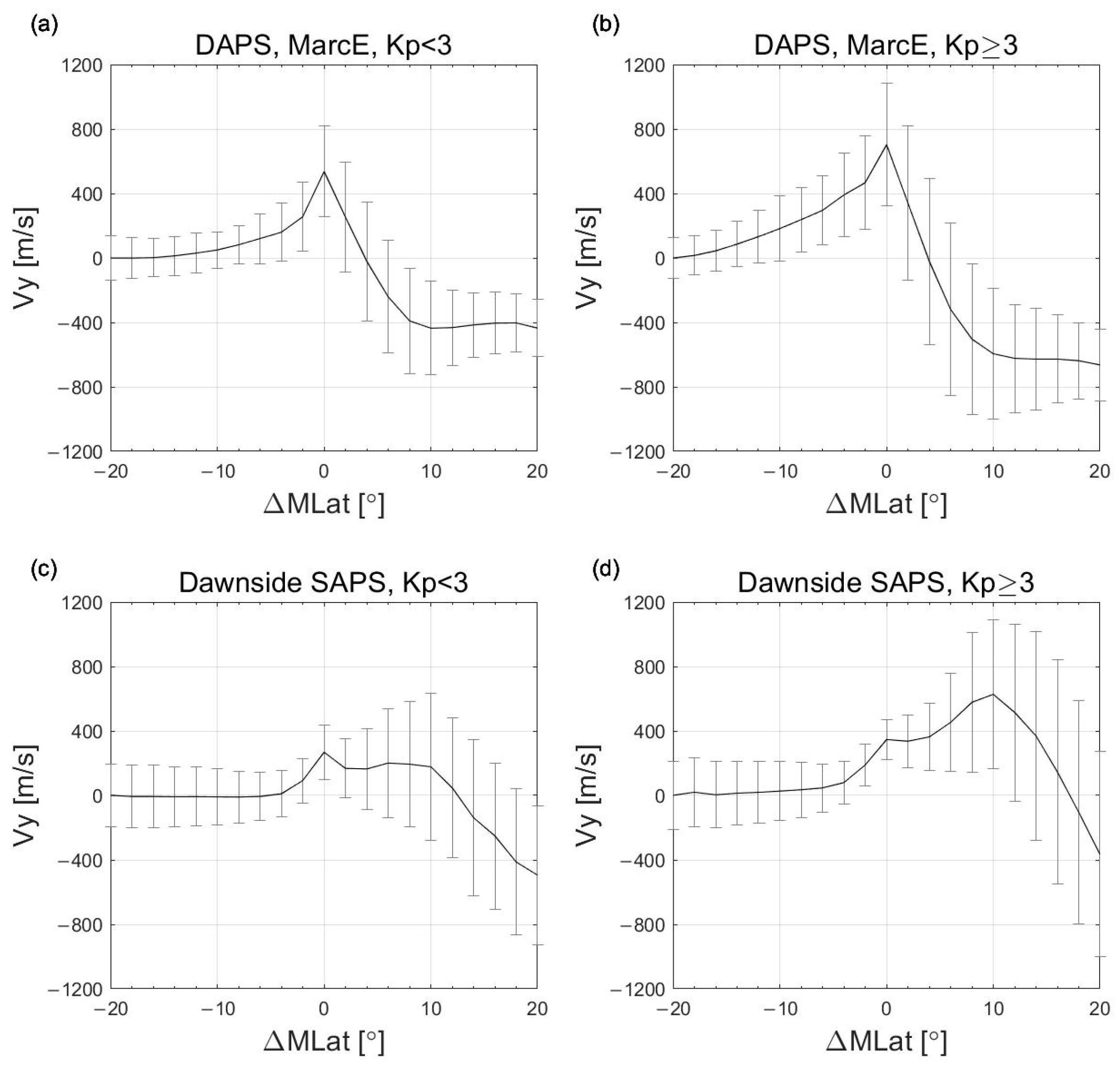
Figure 4.
Superposed epoch analyses of the vertical flow velocity (Vz) for DAPS (a,b) at March equinox and dawnside SAPS events (c,d) without seasonal separation under different geomagnetic activity levels. The 0 key MLat denotes the latitude where the cross−track velocity (DAPS or SAPS) peaks. Positive values denote upward flow. The bars show the standard deviations of 2° averages.

Figure 5.
Superposed epoch analyses of the plasma density (Ne) for DAPS (a,b) at March equinox and dawnside SAPS events (c,d) without seasonal separation under different geomagnetic activity levels. The 0 key MLat denotes the latitude where the cross-track velocity (DAPS or SAPS) peaks. The bars show the standard deviations of 2° averages.
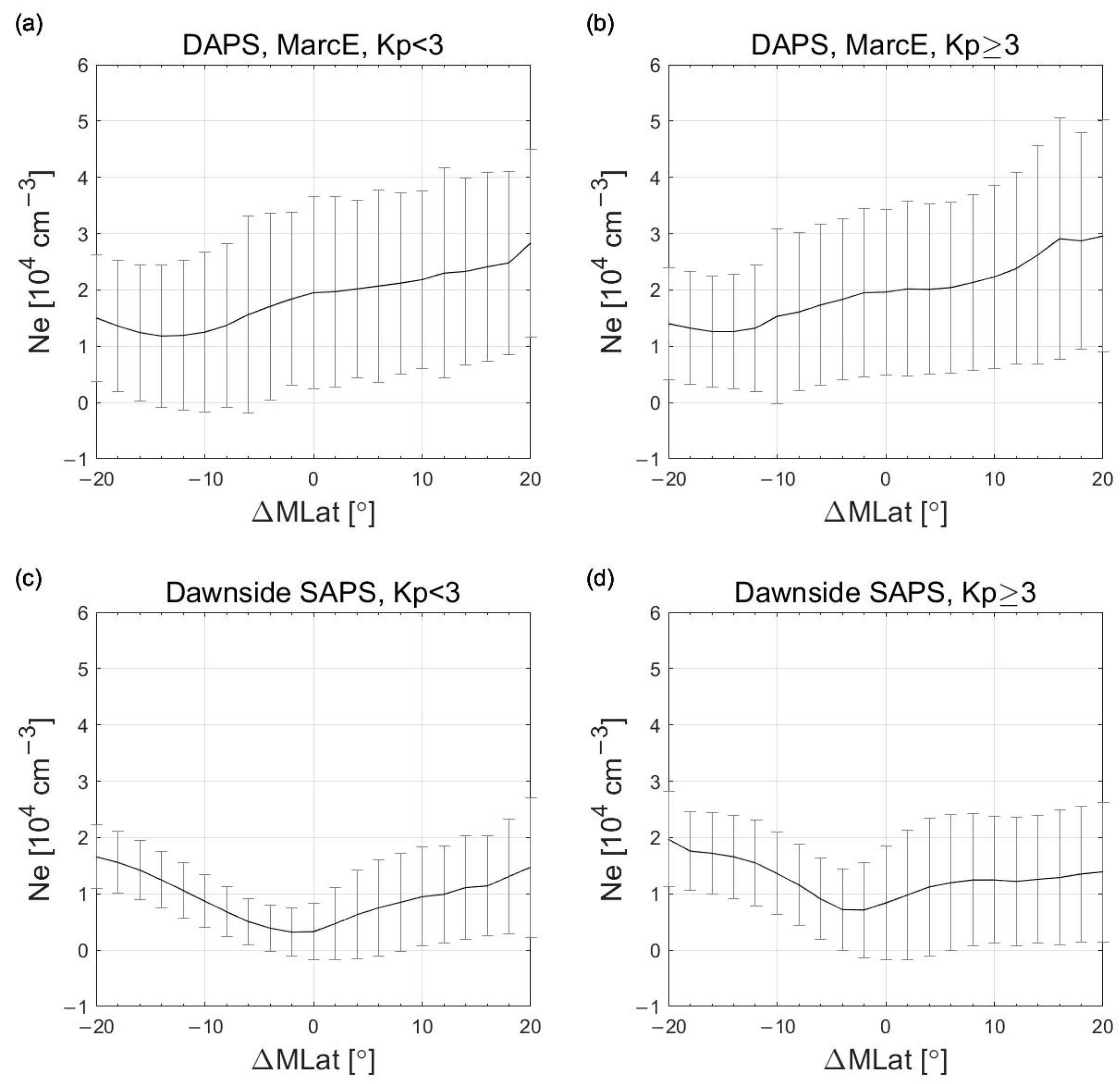
Figure 6.
The event numbers (a) and occurrence frequencies (b) of the SAPS and DAPS as a function of Kp. The black curve is for the DAPS, the blue curve is for the duskside SAPS, and the red curve is for the dawnside SAPS. For DAPS and the duskside SAPS, the scale in the left axis is used, while for the dawnside SAPS, the scale in the right axis is used. The F16 orbit numbers divided by a factor of 4 for better visualization in the dawn and dusk sectors are shown as bars (the scale in the left axis is used).
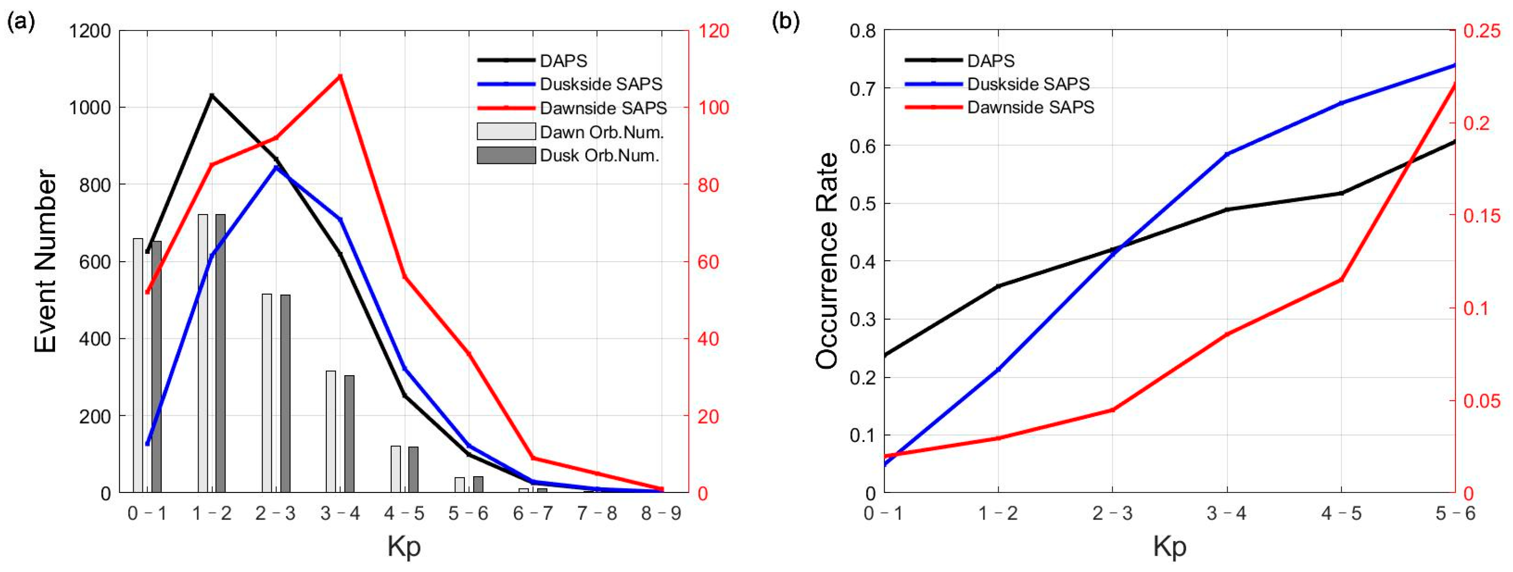
Figure 7.
Correlation of DAPS (a) and SAPS (b) velocity with the upward velocity in the Northern Hemisphere under different geomagnetic activity levels. The correlation coefficient R (DAPS and SAPS), linear fitting line and fitting function (DAPS) are also shown.
Figure 7.
Correlation of DAPS (a) and SAPS (b) velocity with the upward velocity in the Northern Hemisphere under different geomagnetic activity levels. The correlation coefficient R (DAPS and SAPS), linear fitting line and fitting function (DAPS) are also shown.

Figure 8.
Superposed epoch analyses of the ion upward flux for DAPS (a,b) at March equinox and dawnside SAPS events (c,d) without seasonal separation under different geomagnetic activity levels. The 0 key MLat denotes the latitude where the cross-track velocity peaks. The bars show the mean standard deviations of 2° averages.

Figure 9.
Superposed epoch analyses of the ion temperature for DAPS (a,b) at March equinox and dawnside SAPS events (c,d) without seasonal separation under different geomagnetic activity levels. The 0 key MLat denotes the latitude where the cross-track velocity peaks. The bars show the mean standard deviations of 2° averages.
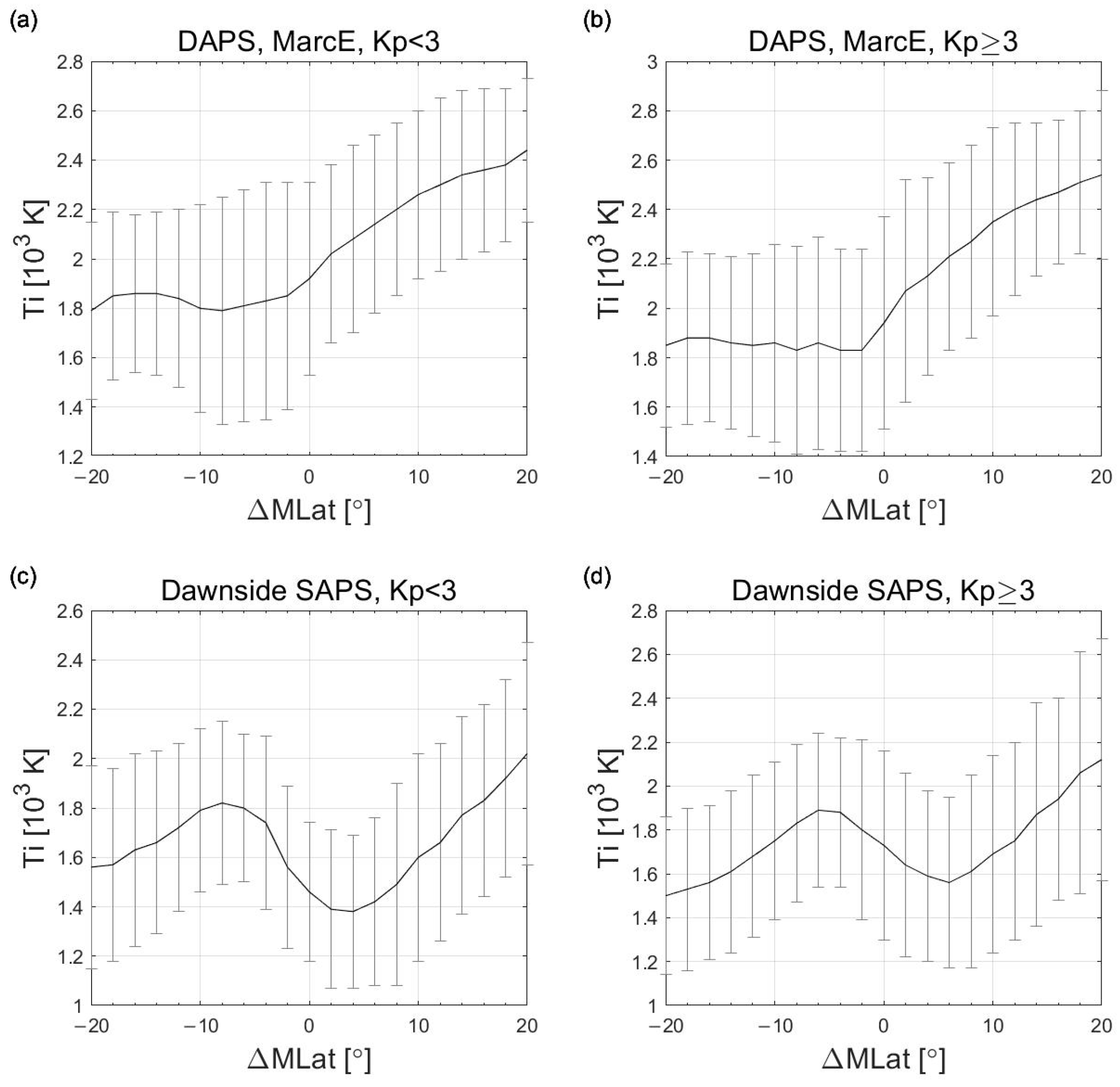
Figure 10.
Superposed epoch analyses of the electron temperature for DAPS (a,b) at March equinox and dawnside SAPS events (c,d) without seasonal separation under different geomagnetic activity levels. The 0 key MLat denotes the latitude where the cross-track velocity peaks. The bars show the mean standard deviations of 2° averages.

Table 1.
The numbers of dawnside SAPS and DAPS events in each season under two different Kp levels. The abbreviation “MarcE” denotes the March equinox, “JuneS” denotes the June solstice, “SeptE” denotes the September equinox, and “DeceS” denotes the December solstice.
Table 1.
The numbers of dawnside SAPS and DAPS events in each season under two different Kp levels. The abbreviation “MarcE” denotes the March equinox, “JuneS” denotes the June solstice, “SeptE” denotes the September equinox, and “DeceS” denotes the December solstice.
| Dawnside SAPS | DAPS | |||||||
|---|---|---|---|---|---|---|---|---|
| Season | Kp < 3 | Kp ≥ 3 | Kp < 3 | Kp ≥ 3 | ||||
| Number of Events | Mean Kp | Number of Events | Mean Kp | Number of Events | Mean Kp | Number of Events | Mean Kp | |
| MarcE | 62 (3.2%) | 1.6 | 69 (13.3%) | 4.2 | 637 (33.1%) | 1.5 | 265 (51.0%) | 3.8 |
| JuneS | 7 (0.4%) | 1.9 | 16 (3.9%) | 4.8 | 597 (30.5%) | 1.4 | 208 (50.2%) | 3.9 |
| SeptE | 82 (4.7%) | 1.4 | 87 (15.0%) | 4.2 | 565 (32.5%) | 1.5 | 305 (52.4%) | 4.1 |
| DeceS | 78 (4.0%) | 1.6 | 43 (9.5%) | 3.8 | 721 (36.8%) | 1.4 | 228 (50.1%) | 3.6 |
Table 2.
The mean velocities of the DAPS and dawnside SAPS at the latitudes where they peak under two different Kp levels. The abbreviation MarcE denotes the March equinox, JuneS denotes the June solstice, SeptE denotes the September equinox, and DeceS denotes the December solstice.
Table 2.
The mean velocities of the DAPS and dawnside SAPS at the latitudes where they peak under two different Kp levels. The abbreviation MarcE denotes the March equinox, JuneS denotes the June solstice, SeptE denotes the September equinox, and DeceS denotes the December solstice.
| Eastward Velocity, Vy (m/s) | DAPS | Dawnside SAPS | |||
|---|---|---|---|---|---|
| Season | MarcE | JuneS | SeptE | DeceS | / |
| Kp < 3 | 536 | 541 | 724 | 717 | 268 |
| Kp ≥ 3 | 704 | 717 | 915 | 807 | 347 |
Table 3.
The mean upflow velocities (Vz) at the latitudes where the DAPS and dawnside SAPS peak under two different Kp levels. The abbreviation MarcE denotes the March equinox, JuneS denotes the June solstice, SeptE denotes the September equinox, and DeceS denotes the December solstice.
Table 3.
The mean upflow velocities (Vz) at the latitudes where the DAPS and dawnside SAPS peak under two different Kp levels. The abbreviation MarcE denotes the March equinox, JuneS denotes the June solstice, SeptE denotes the September equinox, and DeceS denotes the December solstice.
| Upward Velocity, Vz (m/s) | DAPS | Dawnside SAPS | |||
|---|---|---|---|---|---|
| Season | MarcE | JuneS | SeptE | DeceS | / |
| Kp < 3 | 185 | 168 | 273 | 218 | 167 |
| Kp ≥ 3 | 284 | 290 | 384 | 325 | 116 |
Table 4.
The mean plasma density (Ne) at the latitudes where the DAPS and dawnside SAPS peak under two different Kp levels. The abbreviation MarcE denotes the March equinox, JuneS denotes the June solstice, SeptE denotes the September equinox, and DeceS denotes the December solstice.
Table 4.
The mean plasma density (Ne) at the latitudes where the DAPS and dawnside SAPS peak under two different Kp levels. The abbreviation MarcE denotes the March equinox, JuneS denotes the June solstice, SeptE denotes the September equinox, and DeceS denotes the December solstice.
| Plasma Density, Ne (104/cm³) | DAPS | Dawnside SAPS | |||
|---|---|---|---|---|---|
| Season | MarcE | JuneS | SeptE | DeceS | / |
| Kp < 3 | 1.95 | 2.13 | 0.62 | 0.52 | 0.33 |
| Kp ≥ 3 | 1.96 | 1.98 | 0.91 | 0.78 | 0.84 |
Table 5.
The mean ion upward flux at the latitudes where the DAPS and dawnside SAPS peak under two different Kp levels. The abbreviation MarcE denotes the March equinox, JuneS denotes the June solstice, SeptE denotes the September equinox, and DeceS denotes the December solstice.
Table 5.
The mean ion upward flux at the latitudes where the DAPS and dawnside SAPS peak under two different Kp levels. The abbreviation MarcE denotes the March equinox, JuneS denotes the June solstice, SeptE denotes the September equinox, and DeceS denotes the December solstice.
| Upflow Flux (108 cm−2s−1) | DAPS | Dawnside SAPS | |||
|---|---|---|---|---|---|
| Season | MarcE | JuneS | SeptE | DeceS | / |
| Kp < 3 | 2.9 | 3.3 | 1.5 | 0.8 | 0.4 |
| Kp ≥ 3 | 5.1 | 5.3 | 3.6 | 2.3 | 0.7 |
Disclaimer/Publisher’s Note: The statements, opinions and data contained in all publications are solely those of the individual author(s) and contributor(s) and not of MDPI and/or the editor(s). MDPI and/or the editor(s) disclaim responsibility for any injury to people or property resulting from any ideas, methods, instructions or products referred to in the content. |
© 2023 by the authors. Licensee MDPI, Basel, Switzerland. This article is an open access article distributed under the terms and conditions of the Creative Commons Attribution (CC BY) license (https://creativecommons.org/licenses/by/4.0/).
Share and Cite
MDPI and ACS Style
Qian, C.; Wang, H. A Statistical Study of Ion Upflow during Periods of Dawnside Auroral Polarization Streams and Subauroral Polarization Streams. Remote Sens. 2023, 15, 1320. https://doi.org/10.3390/rs15051320
AMA Style
Qian C, Wang H. A Statistical Study of Ion Upflow during Periods of Dawnside Auroral Polarization Streams and Subauroral Polarization Streams. Remote Sensing. 2023; 15(5):1320. https://doi.org/10.3390/rs15051320
Chicago/Turabian StyleQian, Chengyu, and Hui Wang. 2023. "A Statistical Study of Ion Upflow during Periods of Dawnside Auroral Polarization Streams and Subauroral Polarization Streams" Remote Sensing 15, no. 5: 1320. https://doi.org/10.3390/rs15051320
Note that from the first issue of 2016, this journal uses article numbers instead of page numbers. See further details here.