


Stability and Changes in the Spatial Distribution of China’s Population in the Past 30 Years Based on Census Data Spatialization

1
Key Laboratory of Land Surface Pattern and Simulation, Institute of Geographic Sciences and Natural Resources Research, Chinese Academy of Sciences, Beijing 100101, China
2
College of Resources and Environment, University of Chinese Academy of Sciences, Beijing 100049, China
*
Author to whom correspondence should be addressed.
Remote Sens. 2023, 15(6), 1674; https://doi.org/10.3390/rs15061674
Submission received: 17 February 2023
/
Revised: 14 March 2023
/
Accepted: 17 March 2023
/
Published: 20 March 2023
(This article belongs to the Special Issue Remote Sensing Imagery for Mapping Economic Activities)
Abstract
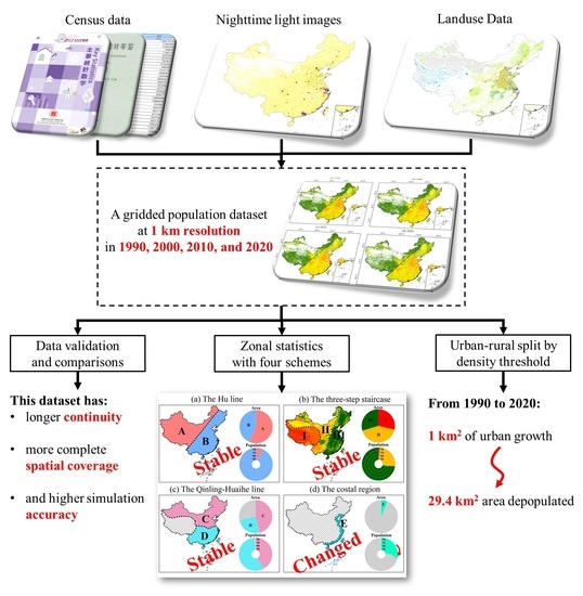
:As the world’s most populous country, China has experienced massive population growth and dramatic regional migration over the past 30 years. From 1990 to 2020, the national population increased by 24.4%, the urban population tripled, and the rural population declined by 41.0%. Combined with complex topographic features, unique characteristics of the population distribution have emerged. Many studies have examined changes in the spatial distribution of the population. However, few studies have examined the stability of certain aspects of this distribution over the last 30 years, particularly at the raster scale, which may provide important information for future research and development plans. Based on land use maps and nighttime light images, China’s census data from 1990 to 2020 was scaled down to a resolution of 1 km using a method called multiple linear regression based on spatial covariates. The results show that there were some striking features of both stability and change in the spatial distribution of China’s population over the past three decades. The population shares divided by the Hu line, the Qinling-Huaihe line, and the three-step staircase have remained almost unchanged. In contrast, the population share of the coastal region has risen from 23.7% to 29.0% during the study period. The urban areas have expanded by 1.35 times and their population has doubled. In addition, for every 1 km2 increase in the urban areas, an area of 29.4 km2 has been depopulated on average. This suggests that urbanization can alleviate population pressure in larger areas. However, the coastal regions and urban and peri-urban areas were the main areas of population density growth, so they required a great deal of attention for ecological protection.
1. Introduction
Over the past three decades, China has experienced rapid urbanization and industrialization [1,2], accompanied by rapid population growth. The national population grew from 1.16 billion in 1990 to 1.44 billion in 2020, an increase of 24.4%. This process has led to a spatial redistribution and reconcentration of the national population. For example, China has experienced a massive migration from rural to urban areas. Between 1990 and 2020, the country’s urbanization rate rose from 26.2% to 63.9%. The urban population has tripled, while the rural population has declined by 41.0% [3,4]. In addition to the trend of migration from rural to urban areas [5,6], other distinctive characteristics of migration have also been noted. This includes the trend of migration from the central and western interior to the southeastern coastal regions [7,8] and from the mountainous areas to the plains [9].
Even though large-scale population movements have occurred, there are still some relatively stable characteristics in the distribution of the population. For example, the population shares on the two sides of the Hu line [10], a traditional dividing line of China’s population density [11], have remained largely stable after more than 80 years of social change [12,13]. On this basis, China’s Premier Li Keqiang has raised the question of whether the Hu line should be broken, whether it can be broken, and how it should be broken [14].
Socioeconomic factors and natural environmental factors both affect the stability and changes in the population distribution. There are significant regional differences in the levels of urbanization and economic development [15,16], which result in variations in population growth and redistribution [17]. On the other hand, natural resources and environmental factors may affect the carrying capacity of the population within a certain region, which can impose constraints on population distribution. Taking topography as an example, China is divided into a three-step staircase, and each step varies greatly in elevation, land cover, and climate [18]. In addition, the Qinling-Huaihe line is regarded as an important geographical dividing line. In existing studies, this line is often used to divide this country into the North and the South of China (Figure 1), since there are great differences between the two sides of this line with respect to climate [19], topography, and many other aspects [20]. In other words, it is necessary to explore the stable and changing aspects of the spatial distribution of China’s population in the past 30 years and the factor(s) that can affect the stability and changes in the population distribution of this country. Studying the long-term trends in population distribution can help us figure out how populations change over time, understand the relationships between population, resources, and the environment, find problems with how resources are used in regional development, and make plans and policies accordingly [21,22,23].
China has conducted seven population censuses since 1949. Census data are relatively accurate for reflecting population size by regions and areas and can provide raw data that are relatively comparable in a time series [24,25]. Many studies have analyzed changes in population shares at scales of regions, provinces, and urban agglomerations over 10- to 20-year periods based on census data [11,12,21,22,26,27,28,29,30]. The population data used in those studies are often at the county or even provincial levels. However, China’s administrative divisions vary greatly in size, with the maximum areas of provincial and county-level administrative regions in mainland China reaching 195 times and 23,800 times the minimum areas, respectively. For the administrative units with a large area, demographic statistics do not reflect the spatial distribution of the population very well, as they may cover a variety of terrains [24]. However, spatially detailed population data is a major input for many natural and socio-economic models, as well as the basis for further research in social and urban sustainability [2] and regional development planning [31]. For example, population datasets are essential for modeling regional climate changes [32,33], land use and urban expansion [34,35], and human well-being [36,37]. They play an important role in other relevant studies of the United Nations [38,39], including their use as indicators for the computation of Sustainable Development Goal 11 [40]. As a result, it is necessary to analyze the distribution patterns of China’s population from statistical units to more fine-grained cells (e.g., raster grids) over the past 30 years.
The spatialization of population data is the process of downscaling data from a lower resolution, usually statistical units, to finer-grained cells. Previous studies have used various methods of spatialization to produce population datasets with high spatial resolution, large areas, and specific time intervals. For example, the Joint Research Center of the European Commission [41] and the Center for International Earth Science Information Network of Columbia University [42] have provided global population density datasets for the years 1975–2020 and 2000–2020, respectively, at 5-year intervals. Although these datasets cover a global scale with a relatively high temporal resolution, the data used for spatialization are not entirely census-based and have larger statistical units [41], thus providing less accuracy in the study area. Meanwhile, some studies have spatialized population data for China in the time periods of pre-2010 [13,26], 2000–2010 [24], and 2000–2020 [21,43]. These datasets lack continuity over a sufficiently long time series to cover the time period of this study, and data are missing in some areas in 2020 (due to the late release of the statistics of China’s 7th census in the Xinjiang region) [43]. Therefore, a spatialized population dataset for China with greater comparability, longer continuity, and more complete spatial coverage is needed for this and other related studies.
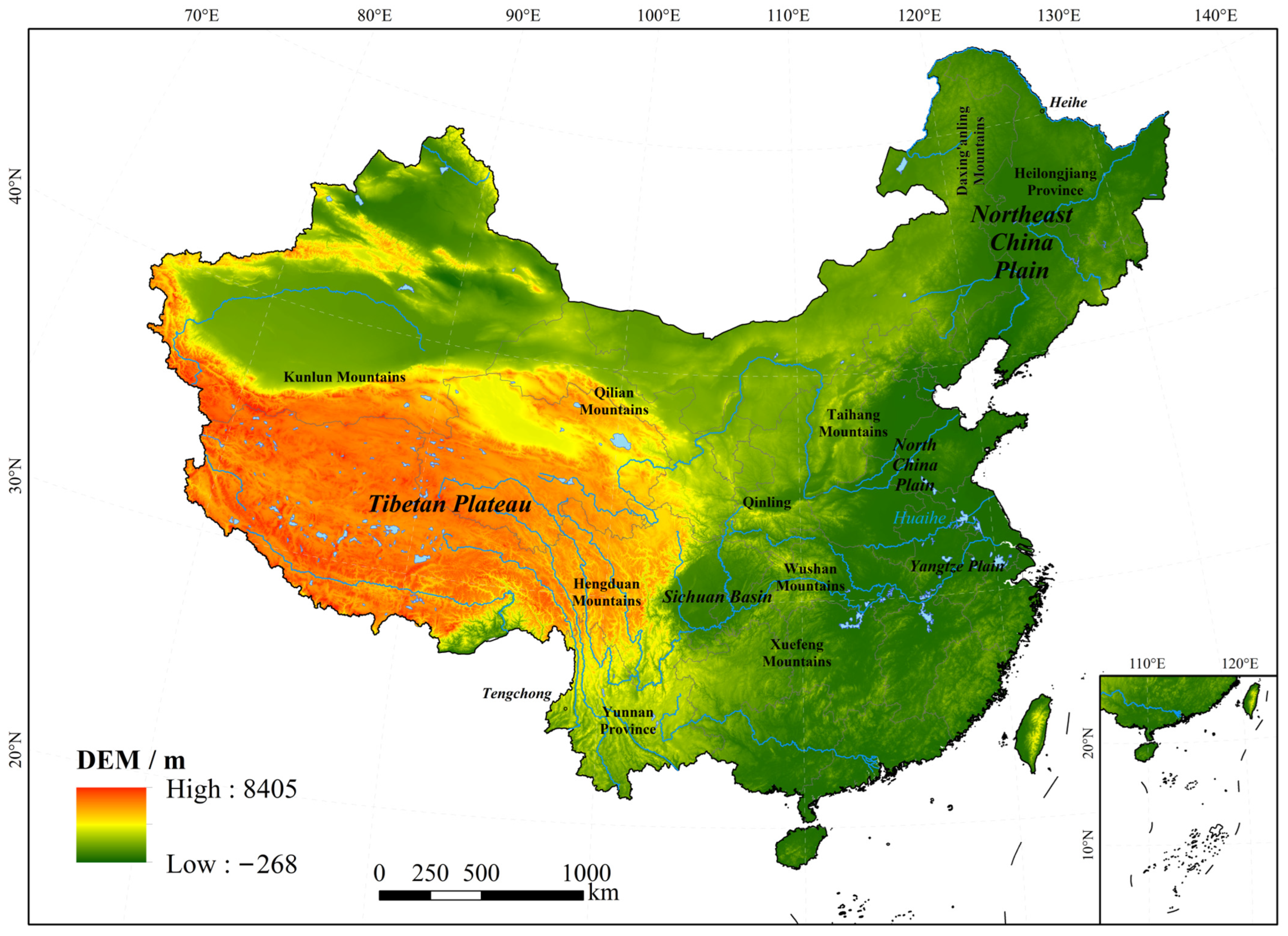
Figure 1.
Natural topography of China with indications of the important toponyms mentioned in this paper.
Figure 1.
Natural topography of China with indications of the important toponyms mentioned in this paper.
There are three main types of methods for spatializing census data [44,45,46,47]: simple area weighting [11,12,21,22,29,48], linear modeling based on spatial covariate weighting [24,26,46], and non-linear modeling [47,49,50]. Among them, the methods of simple area weighting are the simplest, as they simply average the total amount of population onto each grid cell by area. However, the spatial variability of the population distribution within a statistical unit may be ignored. On the other hand, the approaches based on non-linear models, including artificial intelligence modeling, consider complex nonlinear relationships between population distributions and multiple covariates. It may provide higher accuracy, but it makes it difficult to meet their data requirements over a long study period. Finally, the methods of multiple linear regression (MLR) based on spatial covariates have been widely used because of their consistency and comparability across time and because they have relatively high precision [46,47].
Therefore, based on the census, nighttime light (NTL), and land use data, we first used a spatial covariates-based MLR method to spatialize China’s census data at decade intervals from 1990 to 2020 at 1 km grid points. Then, zoning statistics were used to divide the pixel-level population data into four groups based on the Hu line, the three-step staircase, the Qinling-Huaihe line, and the coastal region. Population density thresholds were used to separate urban and rural areas. Next, the aspects of the spatial distribution of China’s population that have changed and those that have remained stable over the past 30 years were examined. Finally, policy implications for urban and regional development, ecological improvement, and resource allocation are provided.
2. Materials and Methods
2.1. Data
2.1.1. Census Data
Population census data were used as the basic data in this study and are listed in Table 1. Population data for Hong Kong and Macau in 1990, 2000, 2010, and 2020 were based on the census results of 1991, 2001, 2011, and 2021, respectively. The population numbers used in this study are for the permanent resident population. These numbers are based on where people lived in the last six months and the results of the census in the same year [51]. The population data at the county level were then matched to the administrative divisions of the corresponding years, as the adjustment of county-level administrative divisions has been frequent and complex in China in the past 30 years.
Population data for some township-level administrative divisions of China’s 6th and 7th censuses were used to validate the spatialization results of the population. The divisions for validation are listed in Table 2.
2.1.2. Nighttime Light (NTL) Data
NTL data, including DMSP/OLS and SNPP/VIIRS images (https://developers.google.com/earth-engine/datasets/catalog, accessed on 1 April 2022), were used to downscale the county-scale population data to the pixel level in this study. The DMSP/OLS images used in this study have been radiance-calibrated based on different satellites and light stages to solve the saturation problem of the sensor. The NTL data were first averaged annually and then resampled onto the resolution of the output population data (1 km). The acquisition and preprocessing of NTL data were carried out on the Google Earth Engine platform. Specifically, the averaged and resampled images from DMSP/OLS in 1992, 2000, and 2010 were employed to spatialize population data in 1990, 2000, and 2010, respectively, and those from SNPP/VIIRS in 2020 (Figure 2) were used to spatialize the population data in 2020. Since the spatialization for each of the four years was processed separately, there was no need to calibrate the four years of data from the different sensors.
2.1.3. Land Use Data
China’s land use data from 1990, 2000, 2010, and 2018 [52] (Figure 3), with a resolution of 100 m, were employed in this study for the population spatialization in 1990, 2000, 2010, and 2020, respectively. The data were visually interpreted mainly based on Landsat images and obtained from the Resource and Environment Science and Data Center, Chinese Academy of Sciences (www.resdc.cn, accessed on 1 April 2022). All cultivated land, water bodies, unused land, and three types of construction land (urban construction land, rural construction land, and other construction land) were employed in this study.
2.2. Spatialization of Population Data
2.2.1. Building the Models for Spatialization with an MLR Model
Previous studies have shown that land use maps and NTL images are highly correlated with human activity and thus can reflect the spatial distribution of the population [24,53,54]. Therefore, based on the land use maps and NTL images of the corresponding years, we first allocated the population census data for administrative division levels onto grid cells, using the MLR method previously described by Tan et al. [24].
The MLR models were constructed at the county scale using census data, mean values of the NTL data, and the area proportions of all cultivated land, urban construction land, rural construction land, and other construction land. The fitting equation for the spatialization of the population in year is as follows:
where represents the population density of county in year ; , , , and represent the area proportions of the cultivated land, urban construction land, rural construction land, and other construction land (hereinafter referred to as “four land classes”) of county in year , respectively; represents the mean value of the NTL data for county in year ; and and are the corresponding weights and intercept terms. The fitting results for each year are shown in Table 3.
2.2.2. Reallocation of Population from the County-Level to 1 km Grid Cells
We used the fitting results in Table 3 to allocate the population onto grid cells with a resolution of 1 km. First, pixels of water areas and unused land were regarded as uninhabited areas in the corresponding years, and the populations of those grid cells were set to zero. Area percentages of the four land classes in each pixel (1 km × 1 km) were then calculated for each year. The results were put into Equation (2) to obtain the simulation results on the pixel level for 1990, 2000, 2010, and 2020.
where represents the population density of pixel in year ; , , , and represent the area proportions of the four land classes of pixel in year , respectively; represents the mean value of the NTL data of pixel in year ; and the values of and are shown in Table 3. Next, the simulation results for the population density for each year were corrected using Equation (3):
where and represent the corrected and uncorrected population densities of pixel in year , represents the total population of county in year , and is the number of pixels in county in year . Finally, the simulation results were validated with the township-level population census data. The validation results reached values of 0.70 and 0.80 for 2010 and 2020, respectively, when verified at the township level. This is better than the WorldPop dataset ( is 0.60 in 2020) [43]. The slopes reached 0.92 and 0.89, respectively (Figure 4), indicating that this method had been tested at the township level with good simulation accuracy.
2.3. Time Period and Regional Divisions
This study analyzed the distribution of China’s population and its regional differences at decade intervals from 1990 to 2020. The four regional divisions are shown in Figure 5.
2.3.1. The Hu Line
The Heihe-Tengchong Line (or the Hu line) is an imaginary line that divides the area of China into two parts with contrasting population densities [10]. It stretches diagonally across China from Heihe, the capital of Heilongjiang Province, in the northeast to Tengchong, the capital of Yunnan Province, in the south (Figure 1). The areas northwest and southeast of the Hu line consist of 57% and 43% of the country’s total area, respectively. In 1935, the part of the Chinese territory (larger than present-day China) southeast of the Hu line accounted for 36% of the total area with 96% of the total population, which illustrates the uneven population distribution of China [10]. From then to 2010, the Hu line could still provide a good overview of the spatial pattern of China’s population [12,13].
2.3.2. The Three-Step Staircase
From the Tibetan Plateau in the southwest to the low-altitude plains along the eastern coast, China’s natural terrain descends gradually as a three-step staircase [18]. The first step is a plateau-alpine region consisting mainly of the Tibetan Plateau. This area reaches an average altitude of over 4000 m and accounts for 29% of the country’s land area. The second step is bounded by the Kunlun Mountains, the Qilian Mountains, and the Hengduan Mountains and descends eastward and northward into a series of plateaus and basins with an average altitude of 1000 to 2000 m. This step contains large arid areas and deserts, accounting for 42% of the national land area. The third step is dominated by plains with a humid monsoon climate and bounded by the Daxing’anling Mountains, the Taihang Mountains, the Wushan Mountains, and the Xuefeng Mountains, with an average elevation of 500 m or less and accounting for about one-quarter of the national land area (Figure 1).
2.3.3. The Qinling-Huaihe Line and the North/South of China
The Qinling-Huaihe line (Figure 1) is an important physical geographic boundary in China. It divides the part of the country outside of the first step into the North and the South [30]. Of the two, the North includes temperate and cold climate zones, covering 46% of the national area, while the South includes subtropical and tropical climate zones, covering 25%. The two parts show great differences in many aspects. For instance, the two parts have very different population growth characteristics [30], agricultural losses [55] from drought and their main causes [19], carbon emissions from household energy use [56], the degree of balanced development in urban and rural areas [20], and whether central heating is provided in winter [57].
2.3.4. The Coastal Region
The coastal region of China is the fastest-growing region of the country’s economy, and it has the highest population inflow. It is also the region most impacted by sea level rise due to global warming and extreme water levels due to high tide levels and storm surges [58,59]. Over 40% of the global population lives within 100 km of the coast, and the share is still rising [60]. From 1975 to 2016, 80% of global deaths due to coastal flooding occurred in that region [61]. For China, about 85% of the area and 89% of the population in the coastal low-lying area, which is more vulnerable to natural disasters and climate change, are located within 100 km of the coastline [62]. Therefore, the land area within 100 km of China’s coastline was defined as the coastal region in this study, and it accounts for 6% of the national area.
2.4. Distinction between Low-, Mid-, and High-Density (Urban) Areas
Previous studies and regulations have put forward some methods to distinguish the different classes of population density. Tan et al. used 200 and 1500 persons/km2 as the thresholds to distinguish between low-, mid-, and high-density regions [24]. For simplicity, this study used 200 and 1500 persons/km2 as the thresholds to distinguish between the low-, mid-, and high-density regions. In addition, a municipal district with a population density of over 1500 persons/km2 is considered the urban area of a city in the 5th national census of China [63]. Therefore, the high-density areas that have a density of over 1500 persons/km2 are considered urban areas in this study.
In conclusion, the census, NTL, and land use data were used to build an MLR-based population spatialization model. The pixel-level population datasets were then obtained with this model. The validation of the data and further analyses, including zonal statistics and the urban-rural split, were then processed. These results in turn provided policy implications for this study. The general flow chart of this study is presented in Figure 6.
3. Results
Based on the methods outlined above, we developed a comparable population raster dataset at 1 km resolution from 1990 to 2020 at decade intervals. Next, we analyzed the characteristics of the changes in the population shares for different geographical regions during the 30 years. The results showed that there were some striking features of both stability and change in the spatial distribution of China’s population in the past three decades (Figure 7).
3.1. Stability of the Spatial Distribution of China’s Population
3.1.1. Population Shares under the Split of the Hu Line
The data indicate that the Hu line was still an important demarcation line for the spatial distribution of China’s population from 1990 to 2020, dividing the nation into two parts with strongly contrasting population densities (Figure 7a). The population density was above 200 persons/km2 for most grid pixels in the area southeast of the line, while it was below 20 persons/km2 for most grid pixels in the northwestern part (Figure 8). Covering about 56.8% of the country’s total area (Figure 5a), the population portion of the northwestern part had no obvious change, increasing from 5.7% to 6.2% in the past 30 years (Figure 7a). The proportions in 2020 and 85 years earlier were similar [10].
3.1.2. Population Shares on the Three-Step Staircase
The population share of each step also changed very little over the past 30 years (Figure 7b). The population share of the first step was the smallest, having increased from 1.0% to 1.2%, while the population share of the third step was the largest, having increased from 71.3% to 72.8% during 1990–2020. Of the three steps, only the population share of the second step has declined over the past 30 years, by 1.7 percentage points.
3.1.3. Population Shares in the North and South of China
The shares of the population in the North and South of China also remained largely stable (Figure 5c). From 1990 to 2020, the northern share of the national population decreased from 42.9% to 40.9%, while the southern share increased from 56.1% to 57.8%. However, the North and the South cover 46.3% and 25.1% of the country’s total area, respectively, so the population density in the North is only about two-fifths of that in the South.
3.2. Changes in the Spatial Distribution of China’s Population
3.2.1. Change in Population Density
During 1990–2020, the population of China grew from 1.16 billion to 1.44 billion, and thus the average population density of the country increased by 24%. In particular, the population density of the South grew more markedly than that of the North, at 28% and 19%, respectively.
In this study, the areas with an absolute population density change of over 10 persons/km2 were considered as the increasing or decreasing density areas (Figure 9). The areas of increasing density were mainly located in and around the large and medium-sized cities. However, the rural areas in the Sichuan Basin, the North China Plain, the Northeast China Plain, and the Yangtze Plain were the concentrated areas of decreasing population density.
From 1990 to 2020, the percentage of the country’s people living in high-density areas went from 26% to 53.5% (Table 4). In contrast, the share of the population located in mid- and low-density regions decreased by 9% and 47%, respectively. From 1990 to 2020, for every 1 km2 increase in high-density areas, 29.4 km2 of the area was depopulated on average.
3.2.2. Changes in Population Share in the Coastal Region of China
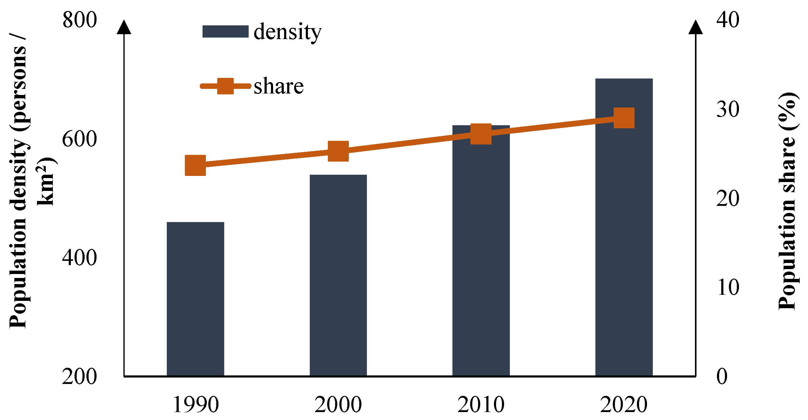
The population share of China’s coastal region showed a clear upward trend during 1990–2020. In 1990, the coastal region carried 23.7% of the population with only 6% of the national land area. By 2020, this share had increased to 29.0%, which was the largest increase among all the geographical divisions (Figure 5d). As a result, the population density of the coastal region increased from 460.1 to 700.7 persons/km2, an increase of 52.3% (Figure 10).
4. Discussion and Policy Implications
This study generated a 1 km resolution population dataset at decade intervals from 1990 to 2020 for China. Compared with other studies on the spatialization of China’s population [13,21,24,26,43], the dataset in this study has a longer temporal continuity and is comparable throughout the time series. Second, unlike previous studies with missing data [21,24,30,43,54], this study collected census data from multiple sources, allowing the output dataset to cover the areas of mainland China, Hong Kong, Macau, and Taiwan, ensuring the most nationwide data completeness. Additionally, the results have been validated at the township level using the census data from 1838 divisions in 2010 and 1796 divisions in 2020 (Table 2), which yielded better validation results for values and slopes (Figure 4) than in previous studies [24] and the WorldPop datasets [43]. In summary, the dataset obtained in this study has longer continuity, more complete spatial coverage, and higher simulation accuracy, thus ensuring a good quantitative depiction of the extent and intensity of the population distribution and variations over the past 30 years.
4.1. Discussion
Some insights can be obtained from the striking features of stability in the spatial distribution of China’s population over the past three decades. (1) The population shares on both sides of the Hu line have not changed very much after nearly 90 years of economic growth and social development, as other studies [11,12] have also found based on the statistics of administrative divisions. Several studies have emphasized that the Hu line has remained generally stable over the past 80 years and is still an important dividing line in China’s demographic geography [12,13,21,29]. These conclusions could respond to the question posed by Premier Li Keqiang [14] that the pattern of China’s population distribution depicted by the Hu line has not been broken and that the current distribution of China’s population is still greatly constrained by topographical factors and the natural background. Since 1999, China’s government has implemented a regional strategic revitalization plan, named “China Western Development”, covering mostly the first and second topographic steps (see Figure 5b). This plan sought to promote rapid economic development and industrialization in the corresponding areas [64] and aimed to slow the outmigration of the population. However, after 20 years of social development, the population shares in the three-step staircase have largely remained stable, so the population goals of this plan were not met. (2) In contrast to the traditional understanding, the consistency of the population shares in the North and the South shows a different trend. Many recent articles [65,66,67] have reported on the migration of China’s population from the north to the south, which is described as “peacocks flying southeast.” However, the population shares of the North and the South have been relatively stable over the past 30 years. This stability is consistent with the findings of previous studies [30] on the population shares of the North and South between 1982 and 2010. Therefore, the natural background still plays a key role in population distribution.
In contrast to the relative stability of certain regions, the changes in population density could provide a scientific basis for ecological construction. For areas with different trends in population density changes, different environmental protection policies should be adopted, and different ecological construction projects should be implemented. (1) The population share of China’s coastal region has increased by five percentage points during the past 30 years (Figure 5d), and its population density has increased by 52.3% (Figure 10). Similarly, the country’s urban areas have expanded 1.35 times, and their share of the population has doubled (Table 4). Several studies have also noted a trend towards population concentration in urban areas [21,22,43], an expansion of high-density (urban) areas [22,24], and an intensification of population inflows in coastal areas [28] and areas around large and medium-sized cities [27,43]. The ecological pressure in these places, including the Yangtze River Delta, the Pearl River Delta, and the Beijing-Tianjin-Hebei region, has increased greatly [68,69,70]. (2) The situation in the mountainous areas of the South is the opposite. Despite the higher overall fertility rate caused by the higher percentage of ethnic minorities [71,72], the populations in these areas have been decreasing in the last decade due to an obvious trend of population emigration. As mass emigration of the populations in the mountainous areas may bring about an improvement in the local vegetation ecology [25,73], the ecological conditions in these areas have improved.
4.2. Policy Implications
The notable features of stability and changes in the spatial distribution of China’s population in the past 30 years may also have some policy implications for regional development and urban planning.
- (1)
- The development of policies and plans should be based on an in-depth understanding of the relationship between people and land; otherwise, achieving their original design objectives will be difficult. Based on respect for the objective law of population distribution and growth, the government can set realistic targets for population development and resource allocation and thus formulate feasible regional and urban development plans.
- (2)
- Areas with rapid population growth, including urban and coastal areas, should receive more attention from the government and scholars. These areas should be the key areas for ecological construction and protection, and important projects and investments related to ecological protection should be more concentrated in these regions.
- (3)
- On the contrary, urbanization may improve the natural environment in vast rural areas by reducing their population pressure. As large numbers of people move into the cities, rural areas should not be the focus of large-scale ecological protection projects at the national level.
5. Conclusions
In this study, based on the census data of 1990, 2000, 2010, and 2020, as well as the regression models established with the proportions of cultivated land and different types of construction land in the land use maps and NTL images as parameters, we developed a continuous and comparable population dataset at 1 km resolution and decadal intervals from 1990 to 2020. We then analyzed the striking features of both stability and change in the spatial distribution of China’s population over the past three decades.
The results showed that the population shares under the splits of the Hu line and the Qinling-Huaihe line, and on the three-step staircase, had remained largely stable over the 30 years, with their shares changing by no more than two percentage points. Among them, the population share northwest of the Hu line increased by only 0.4 percentage points, and that of the South of China increased by 1.8 percentage points. Similarly, the population shares on the three steps of China’s topography did not change noticeably, with the first and third steps increasing by 0.2 and 1.5 percentage points, respectively, and only the second step experiencing a slight decrease.
On the contrary, some geographical divisions experienced large population changes. The population share of the coastal region in the country rose remarkably, by 5.3 percentage points. The shares of the area and population of urban areas increased from 0.5% to 1.3% and from 26.0% to 53.5%, respectively, over the study period. The urban and surrounding areas of large and medium-sized cities were the main areas of population density growth. However, the rural areas in the Great Plains of China experienced a decline in population density.
Finally, and more importantly, for every 1 km2 of urban growth in the country from 1990 to 2020, an average of 29.4 km2 was depopulated.
Author Contributions
Conceptualization, M.T.; methodology, M.T.; software, X.X. and X.L.; validation, X.X.; formal analysis, X.X. and M.T.; data curation, X.X. and X.L.; writing—original draft preparation, X.X.; writing—review and editing, M.T., X.L., X.W. and L.X.; visualization, X.X.; supervision, M.T.; funding acquisition, M.T. All authors have read and agreed to the published version of the manuscript.
Funding
This research was funded by the National Natural Science Foundation of China (grant number: 42271273) and the Third Xinjiang Scientific Expedition Program (grant number: 2021xjkk0902).
Data Availability Statement
The nighttime light data and land use data in this study are accessible publicly, and the URLs are contained within the article.
Conflicts of Interest
The authors declare no conflict of interest.
References
- Wang, Y. Analysis on the evolution of spatial relationship between population and economy in the Beijing-Tianjin-Hebei and Shandong region of China. Sustain. Cities Soc. 2022, 83, 103948. [Google Scholar] [CrossRef]
- Malah, A.; Bahi, H. Integrated multivariate data analysis for Urban Sustainability Assessment, a case study of Casablanca city. Sustain. Cities Soc. 2022, 86, 104100. [Google Scholar] [CrossRef]
- Communiqué of the Fourth National Population Census (No. 1). 1990. Available online: http://www.stats.gov.cn/sj/tjgb/rkpcgb/qgrkpcgb/202302/t20230206_1901990.html (accessed on 16 March 2023).
- Communiqué of the Seventh National Population Census (No. 7). 2021. Available online: http://www.stats.gov.cn/en/PressRelease/202105/t20210510_1817192.html (accessed on 16 March 2023).
- Cai, J.; Wang, G.; Yang, Z. Future trends and spatial patterns of migration in China. Popul. Res. 2007, 31, 9. [Google Scholar]
- Xu, D.; Deng, X.; Huang, K.; Liu, Y.; Yong, Z.; Liu, S. Relationships between labor migration and cropland abandonment in rural China from the perspective of village types. Land Use Policy 2019, 88, 104164. [Google Scholar] [CrossRef]
- Liang, Z.; Ma, Z. China’s floating population: New evidence from the 2000 census. Popul. Dev. Rev. 2004, 30, 467–488. [Google Scholar] [CrossRef]
- Zhu, Y.; Lin, L. Studies on the temporal processes of migration and their spatial effects in China: Progress and prospect. Sci. Geogr. Sin. 2016, 36, 820–828. [Google Scholar]
- Li, S.; Li, X. The mechanism of farmland marginalization in Chinese mountainous areas: Evidence from cost and return changes. J. Geogr. Sci. 2019, 29, 531–548. [Google Scholar] [CrossRef] [Green Version]
- Hu, H.Y. Distribution of Population in China, With Statistics and Maps. Acta Geogr. Sin. 1935, 2, 33–74. [Google Scholar]
- Hu, L.; Liu, Y.; Ren, Y.; Yu, L.; Qu, C. Spatial change of population density boundary in mainland China in recent 80 years. J. Remote Sens. 2015, 19, 928–934. [Google Scholar]
- Li, J.; Lu, D.; Xu, C.; Li, Y.; Chen, M. Spatial heterogeneity and its changes of population on the two sides of Hu Line. Acta Geogr. Sin. 2017, 72, 148–160. [Google Scholar]
- Yang, Q.; Li, L.; Wang, Y.; Wang, X.; Lu, Y. Spatial distribution pattern of population and characteristics of its evolution in China during 1935–2010. Geogr. Res. 2016, 35, 1547–1560. [Google Scholar]
- Lu, D.; Wang, Z.; Feng, Z.; Zeng, G.; Fang, C.; Dong, X.; Liu, S.; Jia, S.; Fang, Y.; Meng, G. Academic debates on Hu Huanyong population line. Geogr. Res 2016, 35, 805–824. [Google Scholar]
- Fang, C.; Liu, X. Temporal and spatial differences and imbalance of China’s urbanization development during 1950–2006. J. Geogr. Sci. 2009, 19, 719–732. [Google Scholar] [CrossRef]
- Deng, X.; Liang, L.; Wu, F.; Wang, Z.; He, S. A review of the balance of regional development in China from the perspective of development geography. J. Geogr. Sci. 2022, 32, 3–22. [Google Scholar] [CrossRef]
- Wang, Q.; Su, M. The effects of urbanization and industrialization on decoupling economic growth from carbon emission—A case study of China. Sustain. Cities Soc. 2019, 51, 101758. [Google Scholar] [CrossRef]
- Hou, H.-Y. Vegetation of China with reference to its geographical distribution. Ann. Mo. Bot. Gard. 1983, 70, 509–549. [Google Scholar] [CrossRef]
- Liang, L.; Zhao, S.-H.; Qin, Z.-H.; He, K.-X.; Chen, C.; Luo, Y.-X.; Zhou, X.-D. Drought Change Trend Using MODIS TVDI and Its Relationship with Climate Factors in China from 2001 to 2010. J. Integr. Agric. 2014, 13, 1501–1508. [Google Scholar] [CrossRef]
- Liu, Y.; Chen, C.; Li, Y. Differentiation regularity of urban-rural equalized development at prefecture-level city in China. J. Geogr. Sci. 2015, 25, 1075–1088. [Google Scholar] [CrossRef]
- Liu, T.; Peng, R.; Zhuo, Y.; Cao, G. China’s changing population distribution and influencing factors: Insights from the 2020 census data. Acta Geogr. Sin. 2022, 77, 381–394. [Google Scholar]
- Mao, Q.; Long, Y.; Wu, K. Spatio-Temporal Changes of Population Density and Urbanization Pattern in China (2000–2010). China City Plan. Rev. 2016, 25, 8–14. [Google Scholar]
- Guan, X.; Wei, H.; Lu, S.; Su, H. Mismatch distribution of population and industry in China: Pattern, problems and driving factors. Appl. Geogr. 2018, 97, 61–74. [Google Scholar] [CrossRef]
- Tan, M.; Li, X.; Li, S.; Xin, L.; Wang, X.; Li, Q.; Li, W.; Li, Y.; Xiang, W. Modeling population density based on nighttime light images and land use data in China. Appl. Geogr. 2018, 90, 239–247. [Google Scholar] [CrossRef]
- Li, S.; Sun, Z.; Tan, M.; Li, X. Effects of rural–urban migration on vegetation greenness in fragile areas: A case study of Inner Mongolia in China. J. Geogr. Sci. 2016, 26, 313–324. [Google Scholar] [CrossRef] [Green Version]
- Gaughan, A.E.; Stevens, F.R.; Huang, Z.; Nieves, J.J.; Sorichetta, A.; Lai, S.; Ye, X.; Linard, C.; Hornby, G.M.; Hay, S.I.; et al. Spatiotemporal patterns of population in mainland China, 1990 to 2010. Sci. Data 2016, 3, 160005. [Google Scholar] [CrossRef] [PubMed] [Green Version]
- Cao, G.; Chen, S.; Liu, T. Changing spatial patterns of internal migration to five major urban agglomerations in China. Acta Geogr. Sin. 2021, 76, 1334–1349. [Google Scholar]
- Wang, X. The Analysis of Evolution of Spatial Pattern of China’s Floating Population and Its Influencing Factors; East China Normal University: Shanghai, China, 2017. [Google Scholar]
- Wang, K.; Deng, Y. Can new urbanization break through the Hu Huanyong Line? Further discussion on the geographical connotations of the Hu Huanyong Line. Geogr. Res. 2016, 35, 11. [Google Scholar]
- Liu, J.; Yang, Q.; Liu, J.; Zhang, Y.; Jiang, X.; Yang, Y. Study on the spatial differentiation of the populations on both sides of the “Qinling-Huaihe Line” in China. Sustainability 2020, 12, 4545. [Google Scholar] [CrossRef]
- UN-DESA. World Population Prospects 2022: Ten Key Messages; UN-DESA: New York, NY, USA, 2022. [Google Scholar]
- Wang, C.; Wang, Z.-H. Projecting population growth as a dynamic measure of regional urban warming. Sustain. Cities Soc. 2017, 32, 357–365. [Google Scholar] [CrossRef] [Green Version]
- Li, J.; Sun, R.; Chen, L. Identifying sensitive population associated with summer extreme heat in Beijing. Sustain. Cities Soc. 2022, 83, 103925. [Google Scholar] [CrossRef]
- Verburg, P.H.; Veldkamp, T.; Bouma, J. Land use change under conditions of high population pressure: The case of Java. Glob. Environ. Change 1999, 9, 303–312. [Google Scholar] [CrossRef]
- Li, Y.; Kong, X.; Zhu, Z. Multiscale analysis of the correlation patterns between the urban population and construction land in China. Sustain. Cities Soc. 2020, 61, 102326. [Google Scholar] [CrossRef]
- Li, S.; Ma, Y. Urbanization, economic development and environmental change. Sustainability 2014, 6, 5143–5161. [Google Scholar] [CrossRef] [Green Version]
- Neil Adger, W. Social Vulnerability to Climate Change and Extremes in Coastal Vietnam. World Dev. 1999, 27, 249–269. [Google Scholar] [CrossRef]
- UN-Habitat. World Cities Report 2022: Envisaging the Future of Cities; UN-Habitat: Nairobi, Kenya, 2022. [Google Scholar]
- UN-DESA. 2018 Revision of World Urbanization Prospects; UN-DESA: New York, NY, USA, 2018. [Google Scholar]
- Report of the Inter-agency and Expert Group on Sustainable Development Goal Indicators (Revised). In Annex IV: Final List of Proposed Sustainable Development Goal Indicators; United Nations Economic and Social Counsil: New York, NY, USA, 2017; Available online: https://sustainabledevelopment.un.org/content/documents/11803Official-List-of-Proposed-SDG-Indicators.pdf (accessed on 26 January 2023).
- Schiavina, M.; Freire, S.; MacManus, K. GHS-POP R2022A—GHS Population Grid Multitemporal (1975–2030). European Commission, Joint Research Centre. 2022. Available online: https://doi.org/10.2905/D6D86A90-4351-4508-99C1-CB074B022C4A (accessed on 29 January 2023).
- Center for International Earth Science Information Network—CIESIN—Columbia University. Gridded Population of the World, Version 4 (GPWv4): Population Density Adjusted to Match 2015 Revision UN WPP Country Totals, Revision 11. 2018. Available online: https://doi.org/10.7927/H4F47M65 (accessed on 29 January 2023).
- Teng, F.; Wang, Y.; Wang, M.; Wang, L. Monitoring and Analysis of Population Distribution in China from 2000 to 2020 Based on Remote Sensing Data. Remote Sens. 2022, 14, 6019. [Google Scholar] [CrossRef]
- Wardrop, N.; Jochem, W.; Bird, T.; Chamberlain, H.; Clarke, D.; Kerr, D.; Bengtsson, L.; Juran, S.; Seaman, V.; Tatem, A. Spatially disaggregated population estimates in the absence of national population and housing census data. Proc. Natl. Acad. Sci. USA 2018, 115, 3529–3537. [Google Scholar] [CrossRef] [Green Version]
- Leyk, S.; Gaughan, A.E.; Adamo, S.B.; de Sherbinin, A.; Balk, D.; Freire, S.; Rose, A.; Stevens, F.R.; Blankespoor, B.; Frye, C. The spatial allocation of population: A review of large-scale gridded population data products and their fitness for use. Earth Syst. Sci. Data 2019, 11, 1385–1409. [Google Scholar] [CrossRef] [Green Version]
- Liu, X.; Xin, L. Assessment of the Efficiency of Cultivated Land Occupied by Urban and Rural Construction Land in China from 1990 to 2020. Land 2022, 11, 941. [Google Scholar] [CrossRef]
- Liu, Z. Dynamic Population Exposure and Anomaly Response Pattern Mining of Typhoon Events Using Big Data; Chinese Academy of Sciences: Beijing, China, 2019. [Google Scholar]
- Holt, J.B.; Lo, C.; Hodler, T.W. Dasymetric estimation of population density and areal interpolation of census data. Cartogr. Geogr. Inf. Sci. 2004, 31, 103–121. [Google Scholar] [CrossRef]
- Robinson, C.; Hohman, F.; Dilkina, B. A deep learning approach for population estimation from satellite imagery. In Proceedings of the 1st ACM SIGSPATIAL Workshop on Geospatial Humanities, Redondo Beach, CA, USA, 7–10 November 2017; pp. 47–54. [Google Scholar]
- Fang, Y.; Jawitz, J.W. High-resolution reconstruction of the United States human population distribution, 1790 to 2010. Sci. Data 2018, 5, 180067. [Google Scholar] [CrossRef] [Green Version]
- Communiqué of the Seventh National Population Census (No. 3). 2021. Available online: http://www.stats.gov.cn/en/PressRelease/202105/t20210510_1817188.html (accessed on 16 March 2023).
- Xu, X.; Liu, J.; Zhang, S.; Li, R.; Yan, C.; Wu, S. China’s Multi-Period Land Use Land Cover Remote Sensing Monitoring Data Set (CNLUCC); Resource and Environment Data Cloud Platform: Beijing, China, 2018. [Google Scholar]
- Sun, W.; Zhang, X.; Wang, N.; Cen, Y. Estimating Population Density Using DMSP-OLS Night-Time Imagery and Land Cover Data. IEEE J. Sel. Top. Appl. Earth Obs. Remote Sens. 2017, 10, 2674–2684. [Google Scholar] [CrossRef]
- Wang, L.; Wang, S.; Zhou, Y.; Liu, W.; Hou, Y.; Zhu, J.; Wang, F. Mapping population density in China between 1990 and 2010 using remote sensing. Remote Sens. Environ. 2018, 210, 269–281. [Google Scholar] [CrossRef]
- Qiang, Z.; Lanying, H.; Jingjing, L.; Qingyan, C. North–south differences in Chinese agricultural losses due to climate-change-influenced droughts. Theor. Appl. Climatol. 2018, 131, 719–732. [Google Scholar] [CrossRef]
- Xu, L.; Qu, J.; Han, J.; Zeng, J.; Li, H. Distribution and evolutionary in household energy-related CO2 emissions (HCEs) based on Chinese north–south demarcation. Energy Rep. 2021, 7, 6973–6982. [Google Scholar] [CrossRef]
- Deng, Y.; Gao, Q.; Yang, T.; Wu, B.; Liu, Y.; Liu, R. Indoor solid fuel use and incident arthritis among middle-aged and older adults in rural China: A nationwide population-based cohort study. Sci. Total Environ. 2021, 772, 145395. [Google Scholar] [CrossRef] [PubMed]
- Fang, J.-Y.; Shi, P.-J. A review of coastal flood risk research under global climate change. Prog. Geogr. 2019, 38, 625–636. [Google Scholar]
- Dasgupta, S.; Wheeler, D.; Bandyopadhyay, S.; Ghosh, S.; Roy, U. Coastal dilemma: Climate change, public assistance and population displacement. World Dev. 2022, 150, 105707. [Google Scholar] [CrossRef]
- The Intergovernmental Oceanographic Commission of UNESCO Enhancing Coastal Resilience during the UN Ocean Decade. Available online: https://www.oceandecade.org/news/enhancing-coastal-resilience-during-the-un-ocean-decade/ (accessed on 26 August 2022).
- Hu, P.; Zhang, Q.; Shi, P.; Chen, B.; Fang, J. Flood-induced mortality across the globe: Spatiotemporal pattern and influencing factors. Sci. Total Environ. 2018, 643, 171–182. [Google Scholar] [CrossRef]
- Shi, M. A Study of Population Distribution and Population Vulnerability to Natural Hazards in Low Elevation Coastal Zone of China. Master’s Thesis, Shanghai Normal University, Shanghai, China, 2012. [Google Scholar]
- Regulations on the Statistical Division of Urban and Rural Areas (for Trial Implementation). Available online: http://www.stats.gov.cn/tjsj/pcsj/rkpc/5rp/html/append7.htm (accessed on 17 September 2022).
- Chen, Y.; Zhang, D. Evaluation and driving factors of city sustainability in Northeast China: An analysis based on interaction among multiple indicators. Sustain. Cities Soc. 2021, 67, 102721. [Google Scholar] [CrossRef]
- Ren, Z. China’s Great Migration Report. 2021. Available online: https://www.yicai.com/news/101077169.html (accessed on 2 October 2021).
- Li, H. Data of 20 Years Prove That “Peacocks Flying Southeast” Uninterrupted. Available online: http://ep.ycwb.com/epaper/ycwb/html/2020-03/17/content_130_245058.htm (accessed on 2 October 2022).
- Kaifeng. Peacocks Flying Southeast! Who Is the Next City of 10 Million People? Available online: https://www.21jingji.com/article/20210609/herald/47f4e2d5fc21f9848b83d1a83632edf9.html (accessed on 2 October 2022).
- Abernethy, V.D. Carrying capacity: The tradition and policy implications of limits. Ethics Sci. Environ. Politics 2001, 2001, 9–18. [Google Scholar] [CrossRef]
- Lane, M. The carrying capacity imperative: Assessing regional carrying capacity methodologies for sustainable land-use planning. Land Use Policy 2010, 27, 1038–1045. [Google Scholar] [CrossRef] [Green Version]
- Wei, Y.; Huang, C.; Lam, P.T.I.; Yuan, Z. Sustainable urban development: A review on urban carrying capacity assessment. Habitat Int. 2015, 46, 64–71. [Google Scholar] [CrossRef]
- Yan, Z.; Hui, L.; Wenbin, J.; Liuxue, L.; Yuemei, L.; Bohan, L.; Lili, W. Third birth intention of the childbearing-age population in mainland China and sociodemographic differences: A cross-sectional survey. BMC Public Health 2021, 21, 2280. [Google Scholar] [CrossRef] [PubMed]
- Zhang, J.; Ding, S.; Hu, X. Analysis of spatial and temporal impact differences of birth rate in mainland China. Sci. Rep. 2022, 12, 17396. [Google Scholar] [CrossRef]
- Li, W.; Tan, M. Spatial redistribution of populations in mountainous areas and its impact on vegetation change in southwest China: A riverside case study. Acta Ecol. Sin. 2018, 38, 8879–8887. [Google Scholar]
Figure 2.
NTL image data for 2020 (from SNPP-VIIRS). Water bodies and unused land have been removed.
Figure 2.
NTL image data for 2020 (from SNPP-VIIRS). Water bodies and unused land have been removed.
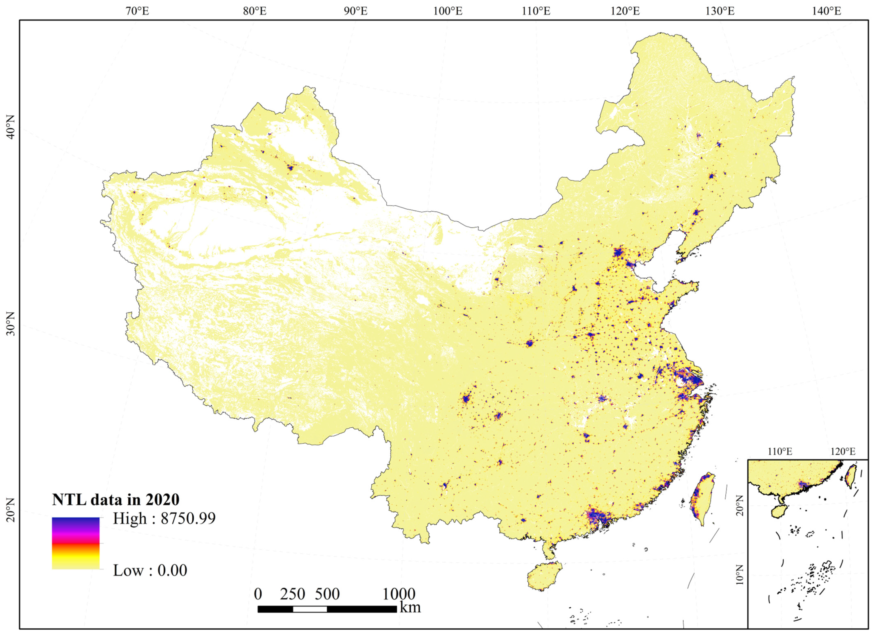
Figure 3.
Land use data for 2018. The land use classes used in this study are cultivated land, water bodies, unused land, and three types of construction land, i.e., urban construction land, rural construction land, and other construction land. Other classes are labeled as colorless.
Figure 3.
Land use data for 2018. The land use classes used in this study are cultivated land, water bodies, unused land, and three types of construction land, i.e., urban construction land, rural construction land, and other construction land. Other classes are labeled as colorless.

Figure 4.
Validation results of the spatialization method in the years 2010 (a) and 2020 (b).

Figure 5.
Regional divisions. Regions A and B in panel (a) represent the areas northwest and southeast of the Hu line; regions I, II, and III in panel (b) represent the first, second, and third steps of China’s natural terrain; regions C and D in panel (c) represent the division of the North and South of China; and region E in panel (d) is the coastal region within 100 km of China’s coastline. The pie graph in the lower left corner of each panel represents the share of each region in the national total.
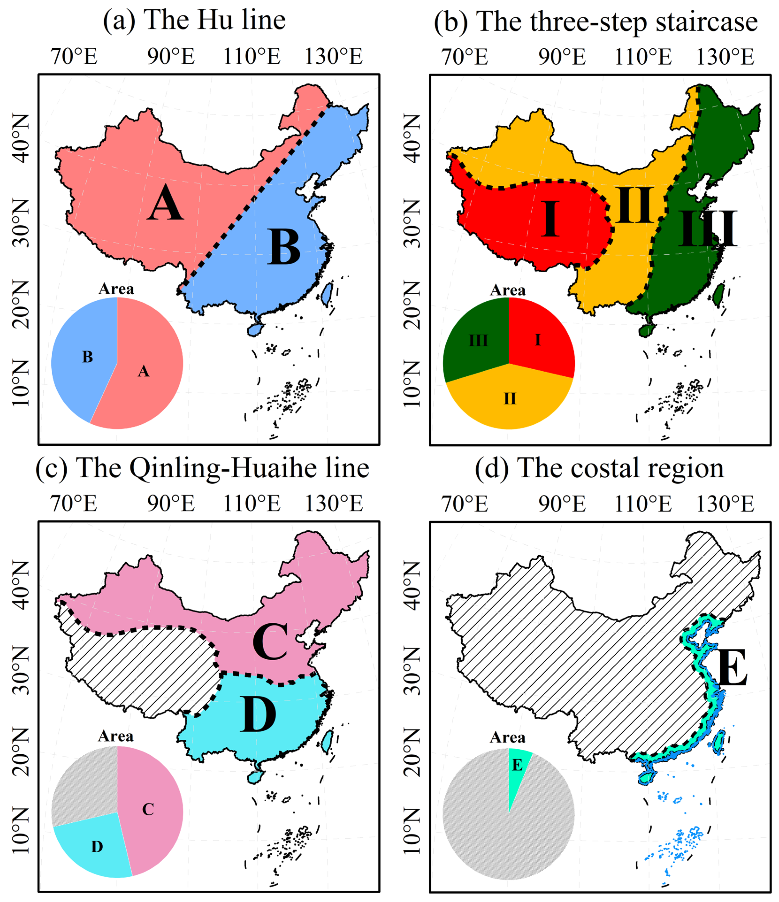
Figure 6.
General flow chart of this study.

Figure 7.
Population shares of each region in the national total. The sector rings A–E and I–III represent the regions in Figure 5 with the same notation.
Figure 7.
Population shares of each region in the national total. The sector rings A–E and I–III represent the regions in Figure 5 with the same notation.
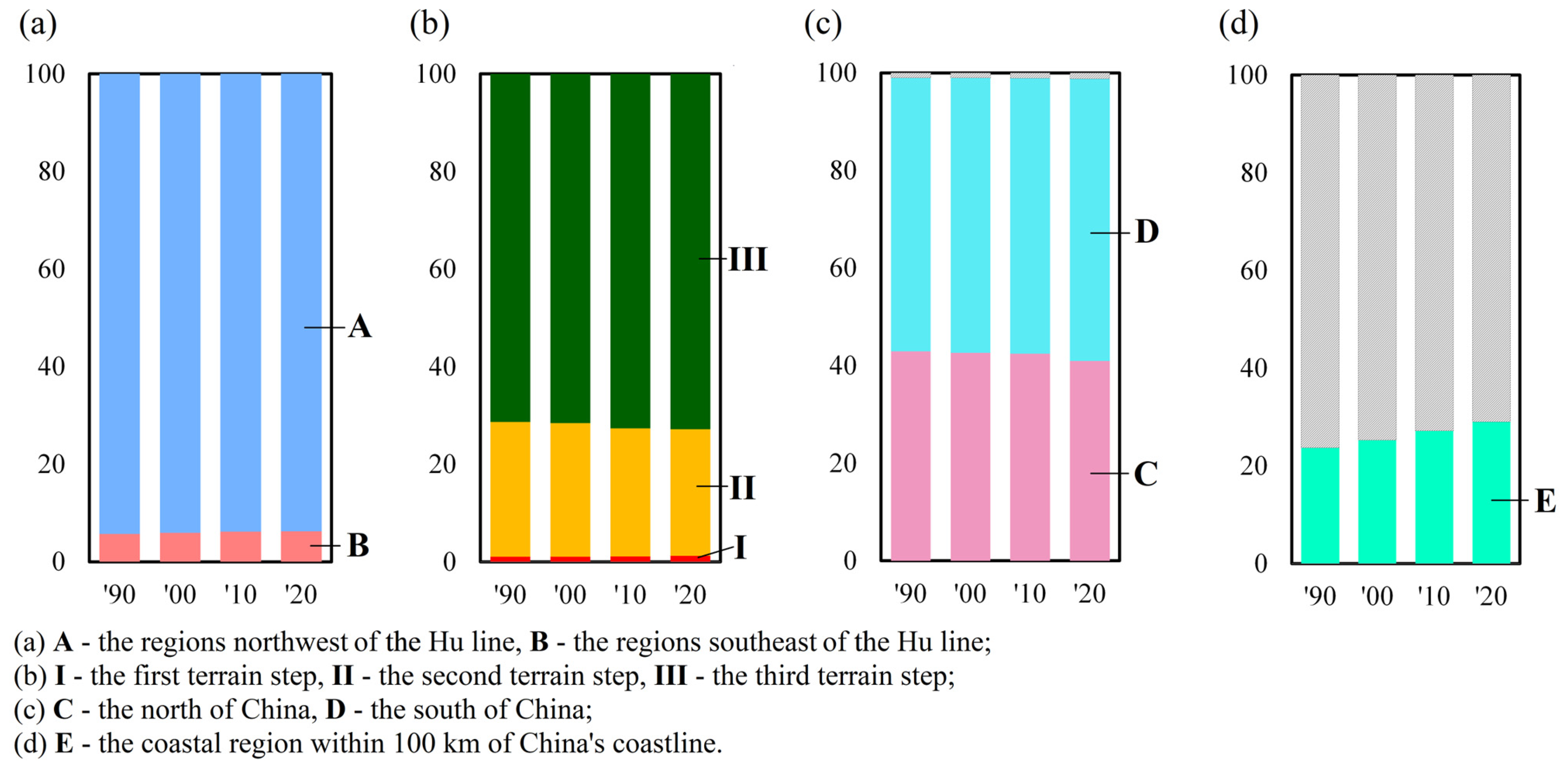
Figure 8.
Population densities in 1990, 2000, 2010, and 2020.
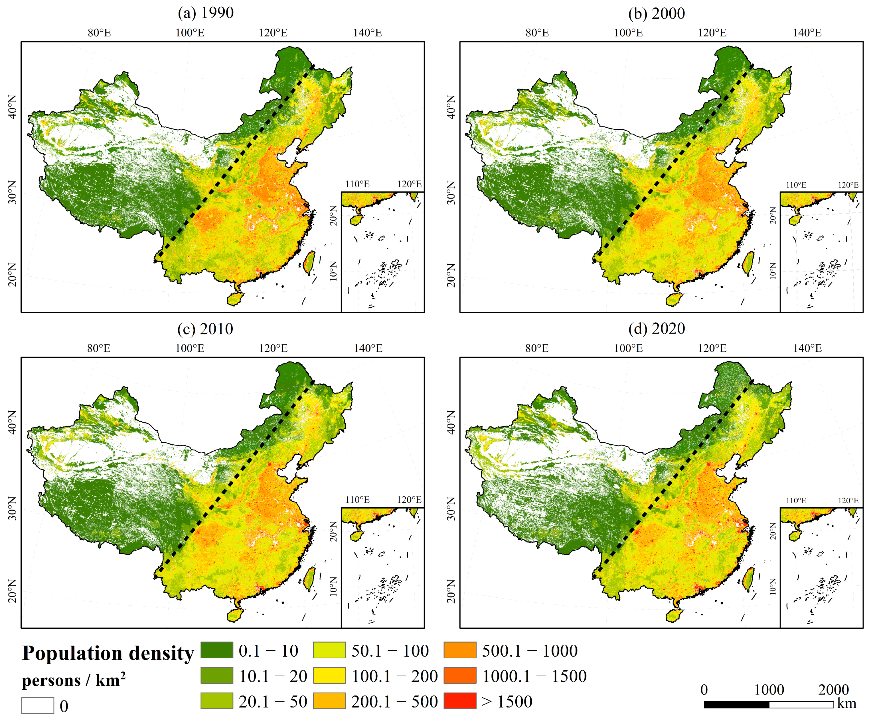
Figure 9.
Changes in population density in China during 1990–2020.

Figure 10.
Changes in the population share and density of China’s coastal region.

Table 1.
Source of population data for the four regions of China.
| Regions | Years | Data Scale | Data Source |
|---|---|---|---|
| Mainland China | 1990, 2000, 2010, 2020 | Prefectural-level for Xinjiang in 2020, county-level for other regions and years | The 4th, 5th, 6th, and 7th National Population Census of China |
| Hong Kong | 1991, 2001, 2011, 2021 | Region-wide | Population census in Hong Kong in 1991, 2001, 2011, and 2021 |
| Macau | 1991, 2001, 2011, 2021 | Region-wide | The 13th, 14th, 15th, and 16th population census in Macau |
| Taiwan Area | 1990, 2000, 2010, 2020 | County-level for 2020, region-wide for other years | Taiwan Population and Housing Census in 1990, 2000, 2010, and 2020 |
Table 2.
List of counties and townships used to validate the results. The numbers of administrative units used for testing differ between 2010 and 2020, as the township-level divisions changed slightly between 2010 and 2020.
Table 2.
List of counties and townships used to validate the results. The numbers of administrative units used for testing differ between 2010 and 2020, as the township-level divisions changed slightly between 2010 and 2020.
| Province-Level Divisions | Cities (Number of Counties in Parentheses) | |
|---|---|---|
| 1 | Beijing Municipality | Beijing (16) |
| 2 | Shanxi Province | Taiyuan (10), Jincheng (6), Shuozhou (6) |
| 3 | Jilin Province | Liaoyuan (4) |
| 4 | Zhejiang Province | Ningbo (10) |
| 5 | Anhui Province | Huainan (7), Suzhou (5) |
| 6 | Hunan Province | Xiangtan (5) |
| 7 | Guangdong Province | Shaoguan (10), Zhaoqing (8), Yangjiang (4), Dongguan (1), Zhongshan (1) |
| 8 | Shaanxi Province | Yulin (12) |
| 9 | Ningxia Hui Autonomous Region | Yinchuan (6), Shizuishan (3), Wuzhong (5), Guyuan (5), Zhongwei (3) |
| County-level divisions | 127 in all. | |
| Township-level divisions | 1838 township-level divisions in 2010, and 1796 township-level divisions in 2020. | |
Table 3.
Fitting results of the weight and intercept terms for each year.
| 1990 | 15.298 | 104.636 | 18.667 | 8.671 | 0.774 | 6.711 | 0.6384 |
| 2000 | 11.791 | 145.668 | 53.877 | 56.129 | 0.046 | 8.473 | 0.8183 |
| 2010 | 11.293 | 133.493 | 37.455 | 66.618 | 0.094 | 8.436 | 0.7466 |
| 2020 | 10.438 | 82.191 | 23.986 | 50.950 | 1.332 | 7.676 | 0.9098 |
Table 4.
Changes in the population density distribution of China in 1990–2020.
| Population Density Regions | Population Density (Persons/km2) * | Area (104 km2) | Population (106 Persons) | ||||||
|---|---|---|---|---|---|---|---|---|---|
| 1990 | 2000 | 2010 | 2020 | 1990 | 2000 | 2010 | 2020 | ||
| Low-density | 0–20 | 314.72 | 297.15 | 291.57 | 273.30 | 16.09 | 15.61 | 16.00 | 16.90 |
| 20–50 | 88.71 | 81.74 | 87.50 | 101.54 | 30.12 | 28.50 | 30.53 | 35.64 | |
| 50–100 | 93.01 | 114.17 | 117.20 | 117.90 | 66.51 | 82.71 | 85.00 | 84.41 | |
| 100–200 | 79.12 | 92.83 | 93.56 | 84.85 | 112.47 | 130.92 | 132.25 | 119.28 | |
| Mid-density | 200–500 | 88.59 | 91.71 | 94.86 | 87.14 | 295.61 | 294.92 | 304.60 | 273.00 |
| 500–1500 | 48.98 | 34.81 | 26.01 | 18.59 | 334.99 | 250.31 | 184.42 | 141.61 | |
| High-density | 1500–3000 | 2.30 | 2.51 | 2.74 | 4.22 | 47.19 | 51.18 | 57.41 | 89.45 |
| >3000 | 2.98 | 3.98 | 5.51 | 8.19 | 253.76 | 417.64 | 553.13 | 682.61 | |
* Population density includes the upper boundary and excludes the lower boundary.
Disclaimer/Publisher’s Note: The statements, opinions and data contained in all publications are solely those of the individual author(s) and contributor(s) and not of MDPI and/or the editor(s). MDPI and/or the editor(s) disclaim responsibility for any injury to people or property resulting from any ideas, methods, instructions or products referred to in the content. |
© 2023 by the authors. Licensee MDPI, Basel, Switzerland. This article is an open access article distributed under the terms and conditions of the Creative Commons Attribution (CC BY) license (https://creativecommons.org/licenses/by/4.0/).
Share and Cite
MDPI and ACS Style
Xu, X.; Tan, M.; Liu, X.; Wang, X.; Xin, L. Stability and Changes in the Spatial Distribution of China’s Population in the Past 30 Years Based on Census Data Spatialization. Remote Sens. 2023, 15, 1674. https://doi.org/10.3390/rs15061674
AMA Style
Xu X, Tan M, Liu X, Wang X, Xin L. Stability and Changes in the Spatial Distribution of China’s Population in the Past 30 Years Based on Census Data Spatialization. Remote Sensing. 2023; 15(6):1674. https://doi.org/10.3390/rs15061674
Chicago/Turabian StyleXu, Xiaofan, Minghong Tan, Xiaoyu Liu, Xue Wang, and Liangjie Xin. 2023. "Stability and Changes in the Spatial Distribution of China’s Population in the Past 30 Years Based on Census Data Spatialization" Remote Sensing 15, no. 6: 1674. https://doi.org/10.3390/rs15061674
Note that from the first issue of 2016, this journal uses article numbers instead of page numbers. See further details here.