
Assessing Shallow Soft Deposits through Near-Surface Geophysics and UAV-SfM: Application in Pocket Beaches Environments

 , , , ,
  and
and
Abstract
:1. Introduction
2. Area of Study
2.1. The Maltese Archipelago
2.2. Case Studies
3. Materials and Methods
3.1. SfM Photogrammetric Survey
3.2. Electrical Resistivity Tomography
3.3. Ambient Seismic Noise Measurements
4. Results
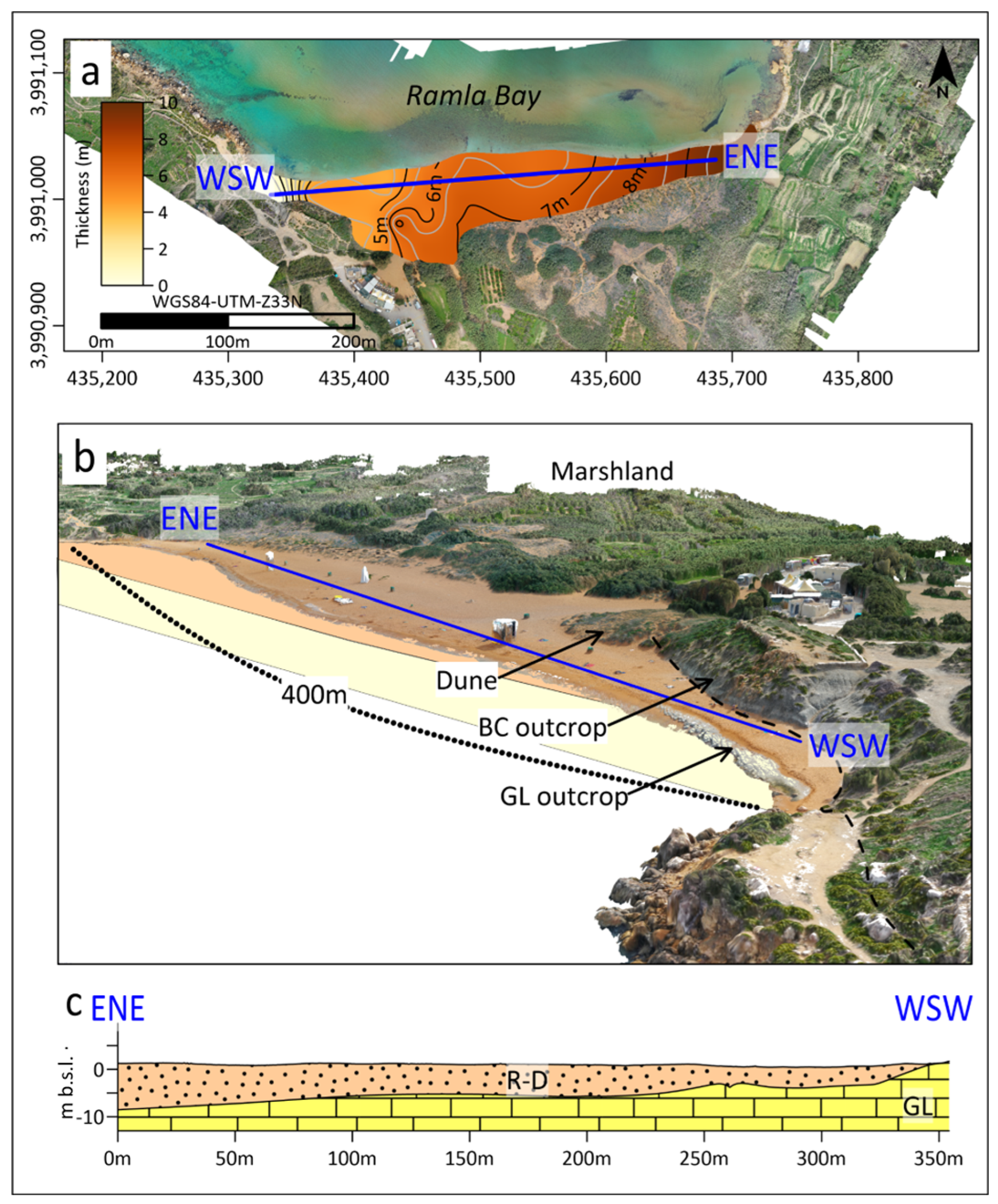
4.1. Photogrammetric Analysis
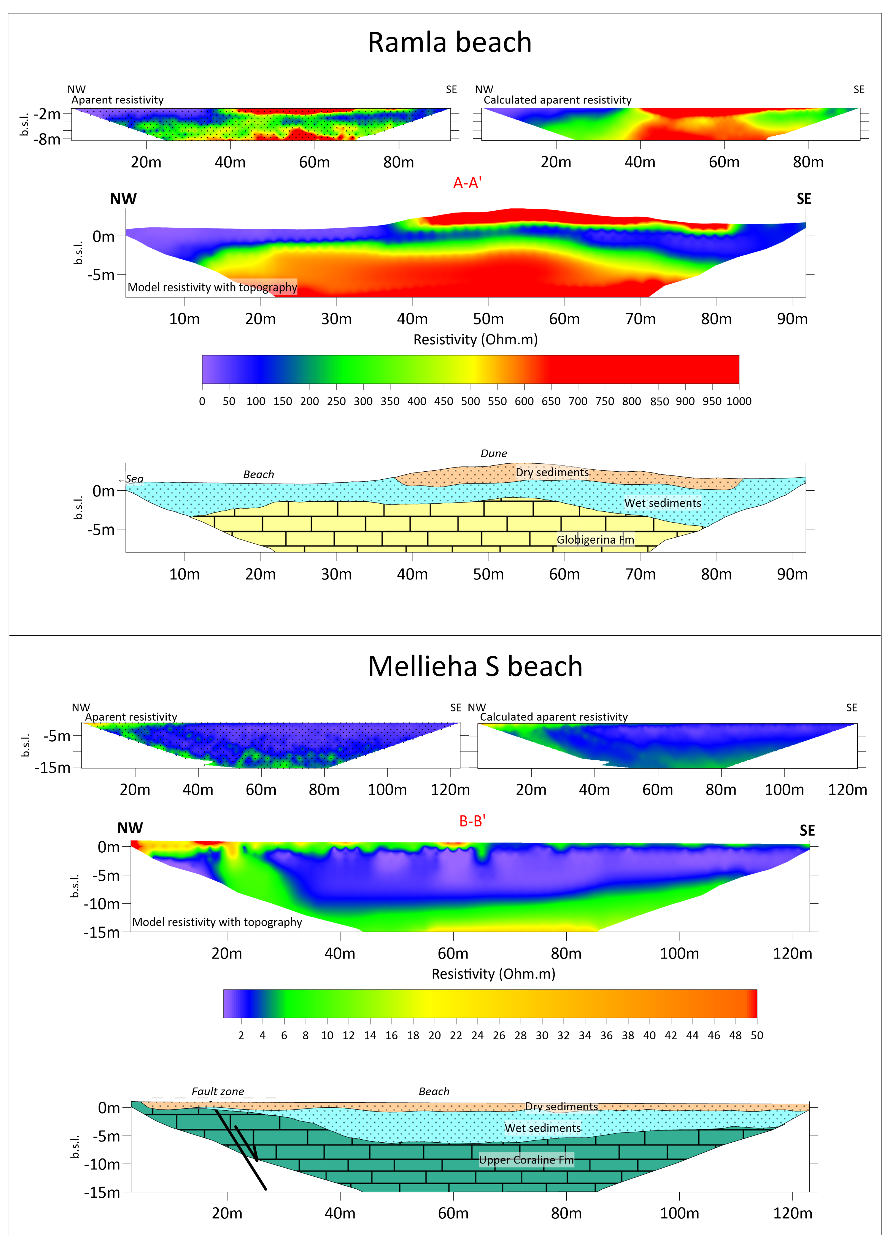
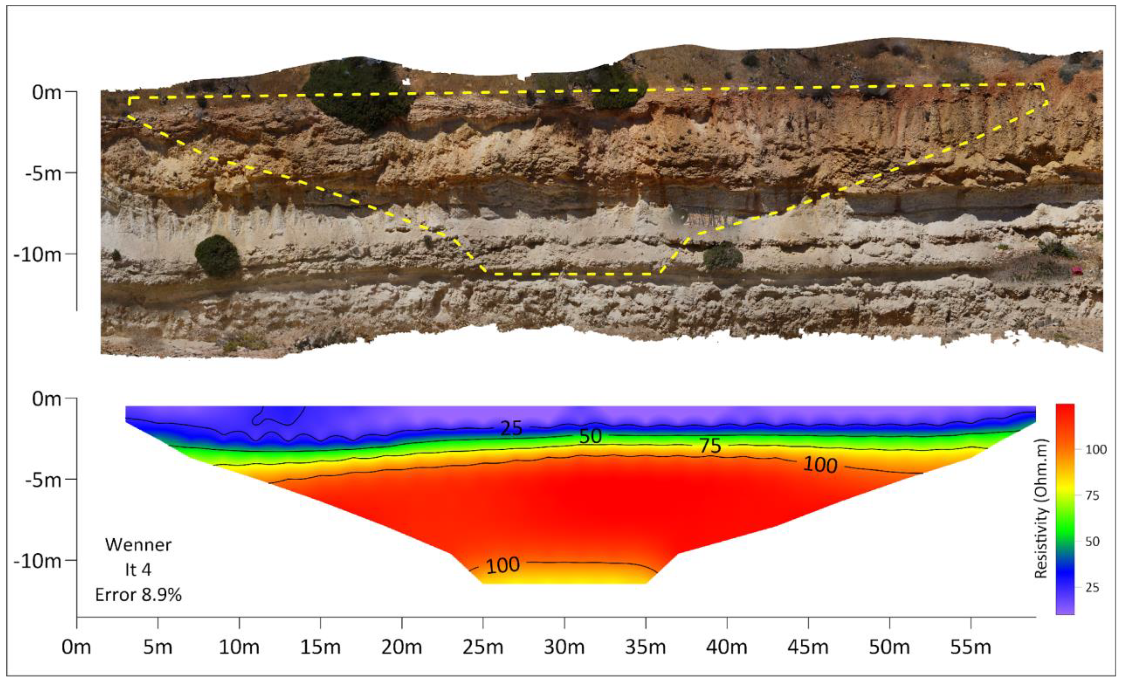
4.2. ERT Results
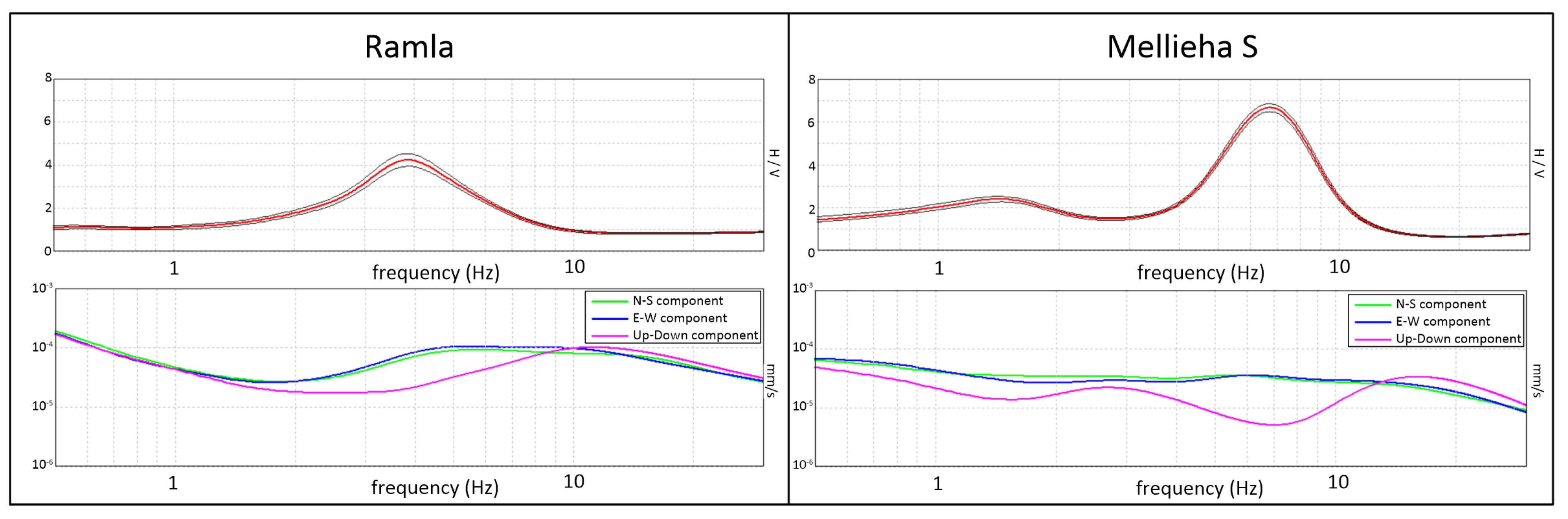
4.3. HVSR Results
4.4. Sediment Thickness Estimation from HVSR
5. Discussion
6. Conclusions
Author Contributions
Funding
Data Availability Statement
Conflicts of Interest
References
- Do, K.; Yoo, J. Morphological Response to Storms in an Embayed Beach Having Limited Sediment Thickness. Estuar. Coast. Shelf Sci. 2020, 234, 106636. [Google Scholar] [CrossRef]
- Cooper, N.J.; Pontee, N.I. Appraisal and Evolution of the Littoral ‘Sediment Cell’Concept in Applied Coastal Management: Experiences from England and Wales. Ocean Coast. Manag. 2006, 49, 498–510. [Google Scholar] [CrossRef]
- Morgan, D.; Gunn, D.; Payo, A.; Raines, M. Passive Seismic Surveys for Beach Thickness Evaluation at Different England (UK) Sites. J. Mar. Sci. Eng. 2022, 10, 667. [Google Scholar] [CrossRef]
- Nakamura, Y. A Method for Dynamic Characteristics Estimation of Subsurface Using Microtremor on the Ground Surface. Railw. Tech. Res. Inst. Q. Rep. 1989, 30, 25–33. [Google Scholar]
- Okada, H.; Suto, K. The Microtremor Survey Method; Society of Exploration Geophysicists: Houston, TX, USA, 2003; ISBN 978-1-56080-174-0. [Google Scholar]
- Villani, F.; D’Amico, S.; Panzera, F.; Vassallo, M.; Bozionelos, G.; Farrugia, D.; Galea, P. Shallow high-resolution geophysical investigation along the western segment of the Victoria Lines Fault (island of Malta). Tectonophysics 2018, 724–725, 220–233. [Google Scholar] [CrossRef]
- Johnson, C.; Lane, J. Statistical Comparison of Methods for Estimating Sediment Thickness from Horizontal-to-Vertical Spectral Ratio (Hvsr) Seismic Methods: An Example from Tylerville, Connecticut, Usa. In Proceedings of the Symposium on the Application of Geophysics to Engineering and Environmental Problems, Denver, CO, USA, 20–24 March 2016; pp. 317–323. [Google Scholar]
- Liang, D.; Gan, F.; Zhang, W.; Jia, L. The Application of HVSR Method in Detecting Sediment Thickness in Karst Collapse Area of Pearl River Delta, China. Environ. Earth Sci. 2018, 77, 259. [Google Scholar] [CrossRef]
- Alonso-Pandavenes, O.; Torres, G.; Torrijo, F.J.; Garzón-Roca, J. Basement Tectonic Structure and Sediment Thickness of a Valley Defined Using HVSR Geophysical Investigation, Azuela Valley, Ecuador. Bull. Eng. Geol. Environ. 2022, 81, 210. [Google Scholar] [CrossRef]
- Mohamed, A.M.E.; El-Hussain, I.; Deif, A.; Al-Jabri, K.; Al-Habsi, Z.; El-Hady, S. Near-Surface Site Characterization at Quriyat City, Sultanate of Oman Using HVSR and MASW Techniques. Arab. J. Geosci. 2015, 9, 23. [Google Scholar] [CrossRef]
- Nelson, S.; McBride, J. Application of HVSR to Estimating Thickness of Laterite Weathering Profiles in Basalt. Earth Surf. Process. Landf. 2019, 44, 1365–1376. [Google Scholar] [CrossRef]
- Nguyen, F.; Jongmans, D.; Pirard, E. Near-Surface Geophysical Imaging and Detection of Slow Active Faults. Ph.D. Thesis, Faculty of Applied Sciences, Liège University, Liège, Belgium, 2005. [Google Scholar]
- Soupios, P.; Papadopoulos, N.; Papadopoulos, I.; Kouli, M.; Vallianatos, F.; Sarris, A.; Manios, T. Application of Integrated Methods in Mapping Waste Disposal Areas. Environ. Geol. 2007, 53, 661–675. [Google Scholar] [CrossRef]
- Danneels, G.; Bourdeau, C.; Torgoev, I.; Havenith, H.-B. Geophysical Investigation and Dynamic Modelling of Unstable Slopes: Case-Study of Kainama (Kyrgyzstan). Geophys. J. Int. 2008, 175, 17–34. [Google Scholar] [CrossRef]
- Benjumea, B.; Macau, A.; Gabàs, A.; Bellmunt, F.; Figueras, S.; Cirés, J. Integrated Geophysical Profiles and H/V Microtremor Measurements for Subsoil Characterization†. Near Surf. Geophys. 2011, 9, 413–425. [Google Scholar] [CrossRef]
- Gallipoli, M.R.; Giocoli, A.; Piscitelli, S. Joint Application of Low-Cost, Fast Executable and Non-Invasive Geophysical Techniques during Emergency and Microzonation Study: Hints from L’Aquila (Italy) Earthquake. In Proceedings of the Geotechnical and Geophysical Site Characterization: Proceedings of the 4th International Conference on Site Characterization ISC-4, Porto de Galinhas, Brazil, 18–21 September 2012; Volume 1, pp. 1477–1484. [Google Scholar]
- Sauret, E.S.G.; Beaujean, J.; Nguyen, F.; Wildemeersch, S.; Brouyere, S. Characterization of Superficial Deposits Using Electrical Resistivity Tomography (ERT) and Horizontal-to-Vertical Spectral Ratio (HVSR) Geophysical Methods: A Case Study. J. Appl. Geophys. 2015, 121, 140–148. [Google Scholar] [CrossRef]
- Abu Zeid, N.; Corradini, E.; Bignardi, S.; Nizzo, V.; Santarato, G. The Passive Seismic Technique ‘HVSR’ as a Reconnaissance Tool for Mapping Paleo-Soils: The Case of the Pilastri Archaeological Site, Northern Italy. Archaeol. Prospect. 2017, 24, 245–258. [Google Scholar] [CrossRef]
- Zarroca, M.; Bach, J.; Linares, R.; Pellicer, X.M. Electrical Methods (VES and ERT) for Identifying, Mapping and Monitoring Different Saline Domains in a Coastal Plain Region (Alt Empordà, Northern Spain). J. Hydrol. 2011, 409, 407–422. [Google Scholar] [CrossRef]
- Colica, E.; D’Amico, S.; Iannucci, R.; Martino, S.; Gauci, A.; Galone, L.; Galea, P.; Paciello, A. Using Unmanned Aerial Vehicle Photogrammetry for Digital Geological Surveys: Case Study of Selmun Promontory, Northern of Malta. Environ. Earth Sci. 2021, 80, 551. [Google Scholar] [CrossRef]
- Furlani, S.; Antonioli, F.; Colica, E.; D’Amico, S.; Devoto, S.; Grego, P.; Gambin, T. Sea Caves and Other Landforms of the Coastal Scenery on Gozo Island (Malta): Inventory and New Data on Their Formation. Geosciences 2023, 13, 164. [Google Scholar] [CrossRef]
- Leucci, G.; Persico, R.; De Giorgi, L.; Lazzari, M.; Colica, E.; Martino, S.; Iannucci, R.; Galone, L.; D’Amico, S. Stability Assessment and Geomorphological Evolution of Sea Natural Arches by Geophysical Measurement: The Case Study of Wied Il-Mielah Window (Gozo, Malta). Sustainability 2021, 13, 12538. [Google Scholar] [CrossRef]
- Bowman, D.; Guillén, J.; López, L.; Pellegrino, V. Planview Geometry and Morphological Characteristics of Pocket Beaches on the Catalan Coast (Spain). Geomorphology 2009, 108, 191–199. [Google Scholar] [CrossRef]
- Dehouck, A.; Dupuis, H.; Sénéchal, N. Pocket Beach Hydrodynamics: The Example of Four Macrotidal Beaches, Brittany, France. Mar. Geol. 2009, 266, 1–17. [Google Scholar] [CrossRef]
- Pranzini, E.; Rosas, V.; Jackson, N.L.; Nordstrom, K.F. Beach Changes from Sediment Delivered by Streams to Pocket Beaches during a Major Flood. Geomorphology 2013, 199, 36–47. [Google Scholar] [CrossRef]
- Turi, A.; Picollo, M.; Valleri, G. Mineralogy and Origin of the Carbonate Beach Sediments of Malta and Gozo, Maltese Islands. Boll. Soc. Ceol. Ital. 1990, J09, 367–374. [Google Scholar]
- Gatt, P. Controls on Plio-Quaternary Foreland Sedimentation in the Region of the Maltese Islands. Boll. Soc. Geol. Ital. 2007, 126, 119–129. [Google Scholar]
- Deidun, A.; Gauci, R.; Schembri, J.A.; Šegina, E.; Gauci, A.; Gianni, F.; Gutierrez, J.A.; Sciberras, A.; Sciberras, J. Comparative Median Grain Size Assessment through Three Different Techniques for Sandy Beach Deposits on the Maltese Islands (Central Mediterranean). J. Coast. Res. 2013, 165, 1757–1761. [Google Scholar] [CrossRef]
- Sammut, S.; Gauci, R.; Drago, A.; Gauci, A.; Azzopardi, J. Pocket Beach Sediment: A Field Investigation of the Geodynamic Processes of Coarse-Clastic Beaches on the Maltese Islands (Central Mediterranean). Mar. Geol. 2017, 387, 58–73. [Google Scholar] [CrossRef]
- Gatt, P. Embayment Morphometrics, Granulometry and Carbonate Mineralogy of Sandy Beaches in the Maltese Islands. Mar. Geol. 2021, 432, 106394. [Google Scholar] [CrossRef]
- Randazzo, G.; Italiano, F.; Micallef, A.; Tomasello, A.; Cassetti, F.P.; Zammit, A.; D’Amico, S.; Saliba, O.; Cascio, M.; Cavallaro, F.; et al. WebGIS Implementation for Dynamic Mapping and Visualization of Coastal Geospatial Data: A Case Study of BESS Project. Appl. Sci. 2021, 11, 8233. [Google Scholar] [CrossRef]
- Farrugia, M.T. Public Perceptions on Coastal Erosion in the Maltese Islands: A Case Study of St George’s Bay (St Julians) and Pretty Bay (Birżebbuġa). Nat. Hazards 2017, 86, 587–604. [Google Scholar] [CrossRef]
- Cooke, B.C.; Jones, A.R.; Goodwin, I.D.; Bishop, M.J. Nourishment Practices on Australian Sandy Beaches: A Review. J. Environ. Manag. 2012, 113, 319–327. [Google Scholar] [CrossRef]
- Pedley, H.M.; House, M.R.; Waugh, B. The Geology of Malta and Gozo. Proc. Geol. Assoc. 1976, 87, 325–341. [Google Scholar] [CrossRef]
- Pedley, H.M. The Ghar Lapsi Limestones: Sedimentology of a Miocene Intra-Shelf Graben; University of Malta Press: Msida, Malta, 1987. [Google Scholar]
- Pedley, M. The Calabrian Stage, Pleistocene Highstand in Malta: A New Marker for Unravelling the Late Neogene and Quaternary History of the Islands. J. Geol. Soc. 2011, 168, 913–926. [Google Scholar] [CrossRef]
- Gauci, M.J.; Deidun, A.; Schembri, P.J. Faunistic Diversity of Maltese Pocket Sandy and Shingle Beaches: Are These of Conservation Value? Oceanologia 2005, 47, 219–241. [Google Scholar]
- Ashby, T. Roman Malta. J. Rom. Stud. 1915, 5, 23–80. [Google Scholar] [CrossRef]
- Mifsud, C. Revisiting Ramla L-Ħamra Villa—New Discoveries and Observations on the Roman Villa Complex in Xagħra, Gozo. Open Archaeol. 2021, 7, 84–97. [Google Scholar] [CrossRef]
- Colica, E.; Galone, L.; D’Amico, S.; Gauci, A.; Iannucci, R.; Martino, S.; Pistillo, D.; Iregbeyen, P.; Valentino, G. Evaluating Characteristics of an Active Coastal Spreading Area Combining Geophysical Data with Satellite, Aerial, and Unmanned Aerial Vehicles Images. Remote Sens. 2023, 15, 1465. [Google Scholar] [CrossRef]
- Everett, M.E. Near-Surface Applied Geophysics; Cambridge University Press: Cambridge, UK, 2013; ISBN 978-1-107-01877-8. [Google Scholar]
- Loke, M.H. Electrical Imaging Surveys for Environmental and Engineering Studies. 1999. Available online: https://pages.mtu.edu/~ctyoung/LOKENOTE.PDF (accessed on 29 October 2023).
- Loke, M.H.; Dahlin, T. A Comparison of the Gauss–Newton and Quasi-Newton Methods in Resistivity Imaging Inversion. J. Appl. Geophys. 2002, 49, 149–162. [Google Scholar] [CrossRef]
- Loke, M.H.; Acworth, I.; Dahlin, T. A Comparison of Smooth and Blocky Inversion Methods in 2D Electrical Imaging Surveys. Explor. Geophys. 2003, 34, 182–187. [Google Scholar] [CrossRef]
- Naudet, V.; Lazzari, M.; Perrone, A.; Loperte, A.; Piscitelli, S.; Lapenna, V. Integrated Geophysical and Geomorphological Approach to Investigate the Snowmelt-Triggered Landslide of Bosco Piccolo Village (Basilicata, Southern Italy). Eng. Geol. 2008, 98, 156–167. [Google Scholar] [CrossRef]
- Mas-Pla, J.; Rodríguez-Florit, A.; Zamorano, M.; Roqué, C.; Menció, A.; Brusi, D. Anticipating the Effects of Groundwater Withdrawal on Seawater Intrusion and Soil Settlement in Urban Coastal Areas. Hydrol. Process. 2013, 27, 2352–2366. [Google Scholar] [CrossRef]
- Bard, P.-Y. Guidelines for the Implementation of the H/V Spectral Ratio Technique on Ambient Vibrations-Measurements, Processing and Interpretations. Available online: https://scholar.google.com/scholar?cluster=14085203609344808715&hl=en&oi=scholarr (accessed on 29 October 2023).
- Buquet, D.; Sirieix, C.; Anschutz, P.; Malaurent, P.; Charbonnier, C.; Naessens, F.; Bujan, S.; Lecroart, P. Shape of the Shallow Aquifer at the Fresh Water–Sea Water Interface on a High-Energy Sandy Beach. Estuar. Coast. Shelf Sci. 2016, 179, 79–89. [Google Scholar] [CrossRef]
- Pischiutta, M.; Villani, F.; D’Amico, S.; Vassallo, M.; Cara, F.; Di Naccio, D.; Farrugia, D.; Di Giulio, G.; Amoroso, S.; Cantore, L.; et al. Results from Shallow Geophysical Investigations in the Northwestern Sector of the Island of Malta. Phys. Chem. Earth Parts A/B/C 2017, 98, 41–48. [Google Scholar] [CrossRef]
- Iannucci, R.; Martino, S.; Paciello, A.; D’Amico, S.; Galea, P. Investigation of Cliff Instability at Għajn Ħadid Tower (Selmun Promontory, Malta) by Integrated Passive Seismic Techniques. J. Seism. 2020, 24, 897–916. [Google Scholar] [CrossRef]
- Ibs-von Seht, M.; Wohlenberg, J. Microtremor Measurements Used to Map Thickness of Soft Sediments. Bull. Seismol. Soc. Am. 1999, 89, 250–259. [Google Scholar] [CrossRef]
- Farrugia, D.; Paolucci, E.; D’Amico, S.; Galea, P. Inversion of Surface Wave Data for Subsurface Shear Wave Velocity Profiles Characterized by a Thick Buried Low-Velocity Layer. Geophys. J. Int. 2016, 206, 1221–1231. [Google Scholar] [CrossRef]
- Bignardi, S. The Uncertainty of Estimating the Thickness of Soft Sediments with the HVSR Method: A Computational Point of View on Weak Lateral Variations. J. Appl. Geophys. 2017, 145, 28–38. [Google Scholar] [CrossRef]
- Journel, A.G.; Rossi, M.E. When Do We Need a Trend Model in Kriging? Math. Geol. 1989, 21, 715–739. [Google Scholar] [CrossRef]
- Kalambet, Y.; Kozmin, Y.; Samokhin, A. Comparison of Integration Rules in the Case of Very Narrow Chromatographic Peaks. Chemom. Intell. Lab. Syst. 2018, 179, 22–30. [Google Scholar] [CrossRef]


| Site | Mellieha Bay | Ramla Bay |
|---|---|---|
| Date | October 2019 | October 2019 |
| Processed images | 573 | 892 |
| Flight altitude | 70 m | 75 m |
| Frontal overlap | 80% | 80% |
| Lateral overlap | 75% | 75% |
| GCPs | 21 | 35 |
| Ramla Bay | Mellieha Bay | |
|---|---|---|
| Point Cloud | ||
| Points | 638,628 of 745,883 | 221,216 of 311,141 |
| RMS reprojection error | 0.178743 (0.928461 pix) | 0.214614 (0.567595 pix) |
| Max reprojection error | 3.86717 (47.1645 pix) | 2.86192 (28.6239 pix) |
| Mean key point size | 4.11674 pix | 2.19475 pix |
| Point colors | 3 bands, uint8 | 3 bands, uint8 |
| Average tie point multiplicity | 4.39553 | 7.87079 |
| Dense Point Cloud | ||
| Points | 81,101,105 | 39,735,110 |
| Point colors | 3 bands, uint8 | 3 bands, uint8 |
| Model | ||
| Faces | 4,937,852 | 2,389,756 |
| Vertices | 2,531,384 | 1,229,757 |
| Vertex colors | 3 bands, uint8 | 3 bands, uint8 |
| Texture | 8096 × 8096, 4 bands, uint8 | 9096 × 9096, 4 bands, uint8 |
| Source data | Dense cloud | Dense cloud |
| DEM | ||
| Size | 29,338 × 22,523; 5.66 cm/px | 23,579 × 27,507; 5.9 cm/px |
| Source data | Dense cloud | Dense cloud |
| Orthomosaic | ||
| Size | 94,923 × 54,443; 1.42 cm/px | 52,139 × 64,799; 1.48 cm/px |
| Colors | 3 bands, uint8 | 3 bands, uint8 |
Disclaimer/Publisher’s Note: The statements, opinions and data contained in all publications are solely those of the individual author(s) and contributor(s) and not of MDPI and/or the editor(s). MDPI and/or the editor(s) disclaim responsibility for any injury to people or property resulting from any ideas, methods, instructions or products referred to in the content. |
© 2023 by the authors. Licensee MDPI, Basel, Switzerland. This article is an open access article distributed under the terms and conditions of the Creative Commons Attribution (CC BY) license (https://creativecommons.org/licenses/by/4.0/).
Share and Cite
Galone, L.; D’Amico, S.; Colica, E.; Iregbeyen, P.; Galea, P.; Rivero, L.; Villani, F. Assessing Shallow Soft Deposits through Near-Surface Geophysics and UAV-SfM: Application in Pocket Beaches Environments. Remote Sens. 2024, 16, 40. https://doi.org/10.3390/rs16010040
Galone L, D’Amico S, Colica E, Iregbeyen P, Galea P, Rivero L, Villani F. Assessing Shallow Soft Deposits through Near-Surface Geophysics and UAV-SfM: Application in Pocket Beaches Environments. Remote Sensing. 2024; 16(1):40. https://doi.org/10.3390/rs16010040
Chicago/Turabian StyleGalone, Luciano, Sebastiano D’Amico, Emanuele Colica, Peter Iregbeyen, Pauline Galea, Lluís Rivero, and Fabio Villani. 2024. "Assessing Shallow Soft Deposits through Near-Surface Geophysics and UAV-SfM: Application in Pocket Beaches Environments" Remote Sensing 16, no. 1: 40. https://doi.org/10.3390/rs16010040