Physics-Informed Deep Learning Inversion with Application to Noisy Magnetotelluric Measurements

Abstract

Despite demonstrating exceptional inversion production for synthetic data, the application of deep learning (DL) inversion methods to invert realistic magnetotelluric (MT) measurements, which are inevitably contaminated by noise in acquisition, poses a significant challenge. Hence, to facilitate DL inversion for realistic MT measurements, this work explores developing a noise-robust MT DL inversion method by generating targeted noisy training datasets and constructing a physics-informed neural network. Different from most previous works that only considered the noise of one fixed distribution and level, we propose three noise injection strategies and compare their combinations to mitigate the adverse effect of measurement noise on MT DL inversion results: (1) add synthetic relative noise obeying Gaussian distribution; (2) propose a multiwindow Savitzky–Golay (MWSG) filtering scheme to extract potential and possible noise from the target field data and then introduce them into training data; (3) create an augmented training dataset based on the former two strategies. Moreover, we employ the powerful Swin Transformer as the backbone network to construct a U-shaped DL model (SwinTUNet), based on which a physics-informed SwinTUNet (PISwinTUNet) is implemented to further enhance its generalization ability. In synthetic examples, the proposed noise injection strategies demonstrate impressive inversion effects, regardless of whether they are contaminated by familiar or unfamiliar noise. In a field example, the combination of three strategies drives PISwinTUNet to produce considerably faithful reconstructions for subsurface resistivity structures and outperform the classical deterministic Occam inversions. The experimental results show that the proposed noise-robust DL inversion method based on the noise injection strategies and physics-informed DL architecture holds great promise in processing MT field data.

1. Introduction

The magnetotelluric (MT) [1,2] method, serving as a non-invasive tool for investigating the Earth’s subsurface, has garnered extensive utilization across various geophysical prospecting scenarios, encompassing crust and upper mantle imaging; geothermal reservoir identification; mineral, oil and gas exploration; etc. Inversion holds a pivotal role in the interpretation of MT measurements (the collected Earth’s natural electric and magnetic fields at its surface). It retrieves the underground resistivity structure from a series of derived apparent resistivity and phase data from the MT measurements. Conventional deterministic inversion methods, such as Gauss–Newton [3,4], Occam [5,6] and nonlinear conjugate gradient [7,8] approaches, have demonstrated favorable outcomes in practice. Nevertheless, these methods employ local search algorithms and are susceptible to the initial model, thus possibly encountering the local minimum problem. Stochastic inversion methods, such as the Bayesian [9] and the quantum genetic [10] approaches, strive to search for the global optimal solution. Unfortunately, these methods entail significant computational costs and, hence, are infrequently adopted to solve geophysical inverse problems in practical tasks.

With the rapid advancement of the deep learning (DL) technique and its recent widespread utilization in geoscience disciplines, applying DL to tackle geophysical inverse problems has emerged as a valuable substitute for conventional inversion methods. The DL-based inversion process generally consists of three stages: training data generation, deep neural network construction and training, and network prediction and subsurface structure imaging. Despite the potentially time-consuming nature of the network training procedure, once adequately performed, the network prediction is extremely efficient, allowing for instant inversion. This characteristic is significantly practical and desirable when processing massive geophysical data and making prompt decisions during field work. Numerous studies have contributed to applying DL techniques in the context of geophysical inverse problems. For instance, Araya-Polo et al. [11] proposed a modular inversion approach based on DL to realize seismic tomography. Das et al. [12] employed a convolutional neural network (CNN) to facilitate seismic impedance inversion. Bai et al. [13] and Wu et al. [14] both used CNNs to perform one-dimensional (1D) airborne transient electromagnetic inversion. Puzyrev and Swidinsky [15] and Moghadas [16] presented 1D DL inversion strategies based on CNNs for electromagnetic and transient electromagnetic induction data. For MT inversion, Ling et al. [17] conducted 1D audio magnetotelluric inversion using deep residual networks. Wang et al. [18] and Liao et al. [19] attempted to invert 2D MT data using CNN and the improved deep belief network, respectively. The DL models in the aforementioned studies are optimized in a completely data-driven way, where the networks derive the mapping relationship between the network input (measurements) and output (geophysical models) directly and solely from the created training dataset. Though a fully data-driven approach can empower DL inversion methods with high automation and is easy to implement, it necessitates constructing a massive representative training dataset to ensure good generalization performance and a robust inversion effect for unfamiliar data, which could pose challenges considering the computational and time costs. To address this issue, a number of more recent works attempted to design physics-informed neural networks (PINNs) or impose priori information constraints to build robust inversion networks. For example, Zhang et al. [20] used seismic data and a priori initial model as one input for network training to perform seismic inversion, partially overcoming the dilemma that the real survey had limited labelled data. Sun et al. [21] and Liu et al. [22] incorporated a forward module modeling the physics of wave propagation into a network training loop, in the form of employing a physics-driven data misfit as the loss function, to achieve unsupervised DL direct current resistivity inversion. Similarly, Liu et al. [23] and Jin et al. [24] coupled the physics-driven data misfit and the data-driven model misfit as the loss function to regulate network training. Nevertheless, though a PINN or a priori information-constrained DL inversion approach has been demonstrated in these works to be more noise-resistant than a completely data-driven one, it still struggles to provide satisfactory outcomes when confronted with geophysical measurements compromised by noise interference.

In realistic exploration scenarios, MT measurements are inevitably corrupted by noise. This unfavorable condition necessitates a more noise-robust DL inversion method to ensure the production of faithful inversion results. Matsuoka [25] mathematically demonstrated that the addition of noise to input data during network back-propagation learning, in some circumstances, can lead to significant improvements in generalization performance. Goodfellow et al. [26] showed that introducing noise to the training data can be adopted to improve the generalization ability of a DL method. Currently, to the best of our knowledge, most existing MT DL inversions use noise-free training data to conduct network training. A few works (e.g., Liu et al. [17] and Liu et al. [27]) have employed the noisy training data to implement MT DL inversion, but they only considered the noise of one fixed distribution and level without further exploration. Hence, in this work, we further explore facilitating DL inversion for noisy MT measurements by introducing noise in training data to train the network. Herein, three strategies and their combinations for adding noise in training data are proposed and compared to develop a robust MT DL inversion method: (1) add synthetic Gaussian distribution noise; (2) propose a multiwindow Savitzky–Golay (MWSG) filtering scheme to extract potential and possible noise from the target field data to be inverted; (3) create an augmented training dataset based on strategies (1) and (2). Moreover, to accurately mine the implicit mapping embedded in data, we introduce Swin Transformer [28,29,30] as the backbone network to design and construct a U-shaped DL model (SwinTUNet), based on which a physics-informed SwinTUNet (PISwinTUNet) is built by integrating MT forward module governing wave propagation in network training loop following Liu et al. [23]. Synthetic and field inversion examples showcase that our noise-robust DL inversion method based on the proposed noise injection strategies and physics-informed DL architecture is expected to be applicable and versatile in realistic MT prospecting scenarios.

2. Problem Statement

Due to the challenges in collecting high-quality realistic MT measurements and associated resistivity models delineating realistic underground structures, synthetic datasets (composed of synthetic resistivity models and the corresponding simulated apparent resistivity and phase data; the former serve as the target output and the latter act as the input) provide a valuable alternative for network training. One commonly used synthetic resistivity model generation method, also employed in this study, is to generate a series of layered resistivity models characterized by smoothly varying resistivity values. The associated simulated apparent resistivity and phase, similar to the ones shown in Figure 1, vary smoothly with the measurement frequencies. However, realistic MT measurements are usually distorted by various types of noise. Though noise reduction methods can be applied to mitigate the adverse effect of noise, it highly depends on domain knowledge and individual experience, and may lead to over-abatement and inevitably increase time and labor burden. Even after noise reduction operation, more often, the denoised MT measurements still contain residual interference. As a result, as displayed in Figure 1, the derived apparent resistivity and phase exhibit fluctuations and irregularities in curves that noticeably deviate from the synthetic ones. This is one of the primary factors that renders DL inversion methods challenging when inverting actual MT data.

To quantitatively illustrate and analyze the inversion performance of deep learning models trained with noise-free datasets on both noise-free and noisy MT data, we conducted the following set of experiments. The data preparation method described in Section 3.3 was used to generate a noise-free training dataset consisting of 800,000 samples (resistivity model-apparent resistivity and phase pairs; the former serves as the target output and the latter act as the input). Likewise, a noise-free test dataset of 20,000 samples was created, and we also generated a noisy test dataset by injecting 5% uniform random noise into this noise-free test dataset. Subsequently, we trained the proposed physics-informed SwinTUNet (PISwinTUNet) (see Section 3.3) using the constructed training datasets of 50,000, 100,000, 200,000, 400,000 and 800,000 samples, respectively, after which the trained networks were loaded to invert both the noise-free and noisy test datasets. Figure 2 shows the model and data misfit (see definitions in Section 3.3) comparison results of the noise-free and noisy test datasets. Evidently, as the training samples grow in number, the model and data misfits of the noise-free test dataset exhibit a gradual decline trend. Conversely, when it comes to the noisy test dataset, the model and data misfits first increase rapidly and then fluctuate around a high of 0.55. The experimental results demonstrate that the DL inversion methods severely degrade in inversion performance when encountering unfamiliar data that are significantly different from the synthetic data for network training, and an increase in training dataset size does not contribute to the improvement of the inversion performance. Hence, in this work, we propose three strategies and their combinations for adding noise in training data to mitigate the adverse effect of noise interference and promote DL inversion application in realistic MT exploration scenarios.

3. Methods

3.1. Neural Network Architecture

In the geophysical community, DL inversion modeling has been dominated by convolutional neural networks. Nevertheless, the receptive field of convolutional kernels is limited, which forces the network to focus on local features and weakens its ability to model long-term dependencies within data. Since 2017, transformers [31] have gained widespread popularity in natural language processing tasks due to their exceptional long-term dependency modeling capability. Very recently, the Swin Transformer (SwinT) [28,29], developed on pure transformer architecture, has been proposed to address vision tasks and shows promising application effect. Presently, SwinTs serve as the backbone network for building DL models across a wide spectrum of visual tasks.

In this work, we introduce SwinT as the backbone network to design and construct a U-shaped DL model SwinTUNet (Figure 3a). To accommodate our 1D MT inverse regression problem, a 1D SwinT block (Figure 3b) is developed by adapting the initial SwinT V2 [29] that was first proposed to solve 2D vision tasks. In our implementation, apparent resistivity and phase are employed as dual-channel input data with a size of $B\times L\times 2$ ($B$, batch size; $L$, length of input data). The resistivity models are used as output data with a size of $B\times R$ ($R$, length of output data). The proposed SwinTUNet is composed of an Encoder module, a Bottleneck layer, a Decoder module and three Skip Connection layers. The Encoder produces hierarchical feature maps with progressively declining resolutions and the Bottleneck layer mines deep feature representations within the data. The Skip Connection layer is designed to integrate shallow and deep-level feature information. The Decoder is intended to perform upsampling and, together with the Encoder, jointly build hierarchical representations. Among these components, the Patch Partition layer splits the input data into nonoverlapping patches ($B\times L/4\times 8$), the Linear Embedding layer maps the feature data to dimension $C$, and two cascading 1D SwinT blocks are responsible for feature extraction and transformation. As depicted in Figure 3b, a 1D SwinT block comprises two consecutive SwinT layers. The first one encompasses a standard 1D window multihead self-attention module (WMSA) and the latter one comprises a 1D shifted window MSA (SW-MSA), both followed by a set of LayerNorm (LN), two-layer multilayer perceptron (MLP) with Gaussian error linear unit nonlinearity [32,33], and residual connection [34,35] modules. With the shifted window partitioning approach, the two consecutive SwinT layers are computed as follows:

$$\begin{array}{l}{\widehat{x}}^n=\mathrm{LN}\left(\mathrm{W}-\mathrm{MSA}\left(x^{n-1}\right)\right)+x^{n-1},\\ x^n=\mathrm{LN}\left(\mathrm{MLP}\left({\widehat{x}}^n\right)\right)+{\widehat{x}}^n,\\ {\widehat{x}}^{n+1}=\mathrm{LN}\left(\mathrm{SW}-\mathrm{MSA}\left(x^n\right)\right)+x^n,\\ x^{n+1}=\mathrm{LN}\left(\mathrm{MLP}\left({\widehat{x}}^{n+1}\right)\right)+{\widehat{x}}^{n+1}\end{array}$$

(1)

where $\widehat{x}$ and $x$ represent the output features. Moreover, the Patch Merging layer performs spatial resolution downsampling. The Patch Expanding layer is developed to enable upsampling without convolution or interpolation, and the Linear Projection layer adjusts the network output to match the output in dimension. In the following implementations, parameters $B$, $C$, $L$ and $R$ are set to 128, 32, 128 and 50, respectively.

3.2. Noisy Injection Strategies

In realistic MT exploration scenarios, the noise can arise from multiple sources, including instrumental errors, various human and environmental factors. Therefore, it is extremely difficult to model all types of noise and then inject them into the training data to improve the inversion performance for noisy MT data. The Central Limit Theorem [36] states that, for a large number of mutually independent random variables, the distribution of their normalized sum approaches a Gaussian distribution as the limit. When dealing with multisource noises, they can be considered as independent random variables with different probability distributions. According to the Central Limit Theorem, as the number of noise sources increases, their normalized sum converges to a Gaussian distribution. Hence, compared to other types or distributions of noise, Gaussian noise does have its rationale. When the source of real noise is complex, Gaussian noise can be regarded as a simple and good analogue of real noise. In this work, we propose three strategies and their combinations for injecting noise in training data based on Gaussian distribution noise and a multiwindow Savitzky–Golay filter.

3.2.1. Strategy One

Add synthetic relative noise of a specific level obeying Gaussian distribution into the training data. In our DL inversion scheme, apparent resistivity and phase data are employed as dual-channel input data. Then, noisy input (apparent resistivity and phase) data can be obtained following:

$$\left\{\begin{array}{l}{{\rho }^{\prime }}_{\mathrm{a}}={\rho }_{\mathrm{a}}\times \left(1+\lambda \times g\right)\\ {\phi }^{\prime }=\phi \times \left(1+\lambda \times g\right)\end{array}\right.$$

(2)

where ${\rho }_{\mathrm{a}}$ and $\phi$ denote the apparent resistivity and phase vector, respectively, $\lambda$ represents the noise level, and $g$ is the pseudo-random number vector following a standard normal distribution with the same size as ${\rho }_{\mathrm{a}}$ or $\phi$.

3.2.2. Strategy Two

We propose a multiwindow Savitzky–Golay (MWSG) filtering scheme to extract potential and possible noise from the target field data to be inverted and then inject the noise into the training data.

The Savitzky–Golay (SG) filter, initially proposed by Savitzky and Golay [37] and renowned for its data smoothing capabilities, has found extensive application in various domains, encompassing geosciences, medicine and analytical chemistry. The SG filter is capable of data smoothing without compromising the retention of valid information. Two pivotal parameters of the SG filter are window size and polynomial order. Typically, optimizing the window size while maintaining a fixed polynomial order is a more appropriate choice. For a given order, a larger window size results in a smoother outcome, albeit at the cost of attenuating sharp fluctuations, whereas a smaller window size permits the SG filter to snugly fit the data but at the expense of sacrificing smoothness. Inspired by this property and characteristic, we propose a multiwindow SG (MWSG) filtering scheme to extract potential and possible noise embedded in the target field data and then introduce them into the training data.

In this study, the polynomial order of the SG filter is set to 3 following the recommendations of Chen et al. [38] and Luo et al. [39]. Consider an actual apparent resistivity data sequence ${\rho }_{\mathrm{a}-\mathrm{actual}}$ and the corresponding phase data sequence ${\phi }_{\mathrm{actual}}$, both of length $L_{\mathrm{actual}}$ (equivalent to the number of acquisition frequencies). Because a longer sequence can ameliorate the deleterious impact of the edge effect of the SG filter [38,40], we apply linear interpolation to transform $\left({\rho }_{\mathrm{a}-\mathrm{actual}},{\phi }_{\mathrm{actual}}\right)$ to $\left({\rho }_{\mathrm{a}-\mathrm{interp}},{\phi }_{\mathrm{interp}}\right)$ of length $L$ (input size of SwinTUNet). As depicted in Figure 4, the procedural steps are detailed below.

• Set the polynomial order $n$ as 3 and predefine the multiple window set $W$ encompassing $m$ windows with different sizes (the window size has to be odd; [39,40]). The window set $W$ can be formulated as:

  $$W:\left\{w_i:2i+1,2\le i\le m\right\}$$

  (3)

  where $w_i$ represents the ith window with a size of $2i+1$. Following Liu et al. [41], the largest window size is set to 65 ($L_{\mathrm{interp}}/2+1$), and thus, the corresponding window number $m$ is 31.
• Randomly select an $\left({\rho }_{\mathrm{a}-\mathrm{actual}},{\phi }_{\mathrm{actual}}\right)$ from the MT field dataset and convert it to $\left({\rho }_{\mathrm{a}-\mathrm{interp}},{\phi }_{\mathrm{interp}}\right)$ using linear interpolation.
• Randomly select a target window $w_i$ from the window set $W$ and apply the SG filter to smooth $\left({\rho }_{\mathrm{a}-\mathrm{interp}},{\phi }_{\mathrm{interp}}\right)$. Express the smoothed $\left({\rho }_{\mathrm{a}-\mathrm{interp}},{\phi }_{\mathrm{interp}}\right)$ as $\left({\rho }_{\mathrm{a}-\mathrm{smooth}},{\phi }_{\mathrm{smooth}}\right)$.
• Extract the potential and possible noise from $\left({\rho }_{\mathrm{a}-\mathrm{interp}},{\phi }_{\mathrm{interp}}\right)$ and $\left({\rho }_{\mathrm{a}-\mathrm{smooth}},{\phi }_{\mathrm{smooth}}\right)$ following:

  $$\left\{\begin{array}{l}nois{e}_{\rho }=\frac{{\rho }_{\mathrm{a}-\mathrm{interp}} - {\rho }_{\mathrm{a}-\mathrm{smooth}}}{{\rho }_{\mathrm{a}-\mathrm{smooth}}}\\ nois{e}_{\phi }=\frac{{\phi }_{\mathrm{interp}} - {\phi }_{\mathrm{smooth}}}{{\phi }_{\mathrm{smooth}}}\end{array}\right.$$

  (4)

  where $nois{e}_{\rho }$ and $nois{e}_{\phi }$ denote the extracted noises from the actual apparent resistivity and phase data, respectively.
• Generate a noise-free synthetic training sample following the data preparation method described in the following Section 3.3, and obtain the noisy training input data by adding the extracted noises $nois{e}_{\rho }$ and $nois{e}_{\phi }$ in the apparent resistivity and phase data following:

  $$\left\{\begin{array}{l}{{\rho }^{\prime }}_{\mathrm{a}}={\rho }_{\mathrm{a}}\left(1+nois{e}_{\rho }\right)\\ {\phi }^{\prime }=\phi \left(1+nois{e}_{\phi }\right)\end{array}\right.$$

  (5)

  where ${{\rho }^{\prime }}_{\mathrm{a}}$ and ${\phi }^{\prime }$ denote the noisy apparent resistivity and phase data, respectively.
• Repeat steps 2 to 5 until the noisy training dataset is built.

3.2.3. Strategy Three

Duplicate the noise-free synthetic training dataset. Then, use strategy one to add Gaussian relative noise with different noise levels ($\lambda$), or/and strategy two to add the extracted potential and possible noise from the target field data, in the apparent resistivity and phase data. Then, combine these noisy apparent resistivity and phase datasets to create an augmented noisy training dataset.

3.3. DL Inversion Scheme

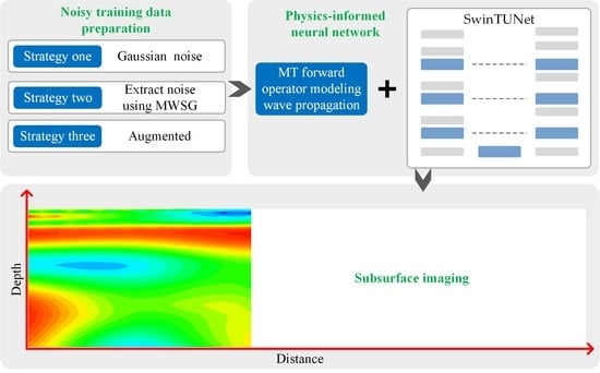
As depicted in Figure 5, the proposed noise-robust DL MT inversion workflow based on a physics-informed neural network model is composed of three stages: noisy training dataset creation, PISwinTUNet building, and inversion and subsurface imaging.

During stage 1, we first applied cubic spline interpolation to generate 100,000 layered resistivity models characterized by smoothly varying resistivity values. Each model comprises 50 layers, with layer thicknesses determined in accordance with Liu et al. [23]. Within the target depth of 10 km, there are 44 layers, while an additional five extended layers are distributed between the target depth and the bottom depth of 50 km. The 50th layer, beneath 50 km, is a homogeneous half-space with infinite thickness. The resistivity values assigned to these 50 layers spanned logarithmically from 1 to 10,000 $\Omega \mathrm{m}$. Subsequently, the apparent resistivity and phase responses were computed for these resistivity models by MT forwarding using a spectrum of 64 frequencies ranging from 0.001 to 1000 Hz. Given that the input size of network was specified as 128, the apparent resistivity and phase sequences were linearly interpolated to match this length. Consequently, a noise-free synthetic dataset, denoted as NoiseFree, was created for network training and validation. This dataset encompasses 100,000 samples, with each sample representing one distinct response–model pair.

Then, the proposed three noise injection strategies were used to prepare noisy training datasets based on the created dataset NoiseFree. For comparison in the following synthetic data inversion examples, we triplicated the dataset NoiseFree to generate three noisy training datasets using noise injection strategy one, named Gaussian1%, Gaussian2% and Gaussian3%, which were contaminated by Gaussian relative noise at 1%, 2% and 3% levels, respectively. Based on the noise injection strategy three, we combined these three datasets to generate an augmented noisy training dataset, named AugGaussian. In the following field data inversion example, noise injection strategy two was employed to extract the potential and possible noise from the MT field data and, together with the other two noise injection strategies, to create a target-oriented noisy training dataset.

During stage 2, we implemented a PINN to establish the mapping from the apparent resistivity and phase to the resistivity model. In this framework, the forward operator, governing MT wave propagation, becomes an integral part in the network training loop, manifesting as a combination of data-driven model misfit and physics-driven data misfit in the form of a loss function. This type of PINN, as previously demonstrated by Liu et al. [23], is designed to adhere to the underlying physical principles of the inverse problem. It results in the construction of more robust networks with superior generalization capabili-ties compared to fully data-driven approaches. In this study, the model misfit ${\zeta }_{\mathrm{model}}$ quantifies the disparities between the predicted resistivity model $\widehat{\rho }$ and the expected re-sistivity model $\rho$, and the data misfit ${\zeta }_{\mathrm{data}}$ quantifies the differences between the orig-inal noise-free input data $d$ (original noise-free rather than noisy apparent resistivity ${\rho }_{\mathrm{a}}$ and phase $\phi$) and the MT responses $\widehat{d}$ (${\widehat{\rho }}_{\mathrm{a}}$ and $\widehat{\phi }$) computed from $\widehat{\rho }$. The formulation of the loss function is as below:

$$\begin{array}{cc}\hfill \Gamma \left(d,\rho ,\theta \right)& ={\zeta }_{\mathrm{model}}\left(\widehat{\rho },\rho \right)+{\zeta }_{\mathrm{data}}\left(\widehat{d},d\right)\hfill \\ \hfill & =\sqrt{\frac{1}{TM}{\displaystyle \sum _{i=1}^T{\displaystyle \sum _{j=1}^M{\left({\widehat{\rho }}_{ij}-{\rho }_{ij}\right)}^2}}}+\sqrt{\frac{1}{TN}{\displaystyle \sum _{i=1}^T{\displaystyle \sum _{j=1}^N{\left({\widehat{d}}_{ij}-d_{ij}\right)}^2}}}\hfill \\ \hfill & =\sqrt{\frac{1}{TM}{\displaystyle \sum _{i=1}^T{\displaystyle \sum _{j=1}^M{\left(\mathrm{Net}{\left(d,\theta \right)}_{ij}-{\rho }_{ij}\right)}^2}}}+\sqrt{\frac{1}{TN}{\displaystyle \sum _{i=1}^T{\displaystyle \sum _{j=1}^N{\left(\mathrm{Forw}{\left(\mathrm{Net}\left(d,\theta \right)\right)}_{ij}-d_{ij}\right)}^2}}}\hfill \end{array}$$

(6)

where $\mathrm{Net}$ symbolizes the trained network parameterized by $\theta$, $\mathrm{Forw}$ corresponds the MT forwarding operation, $T$ represents the training sample number, and $M$, $N$ denote the lengths of the output and input sequences, respectively. Additionally, ${\zeta }_{\mathrm{model}}$ and ${\zeta }_{\mathrm{data}}$ also serve as the evaluation metrics in the subsequent synthetic examples. In the course of the training process, eighty percent of samples were allocated for network training, with the remaining reserved for validating. The input ${\rho }_{\mathrm{a}}$, $\phi$ and expected output $\rho$ were normalized using

$$\left\{\begin{array}{l}{\tilde{\rho }}_{\mathrm{a}}=\frac{{\rho }_{\mathrm{a}} - {\mu }_0}{{\sigma }_0}\\ \tilde{\phi }=\frac{\phi - {\mu }_1}{{\sigma }_1}\\ \tilde{\rho }=\lg \left(\rho \right)\end{array}\right.$$

(7)

where ${\mu }_0$ and ${\sigma }_0$ are the average and standard deviation of ${\rho }_{\mathrm{a}}$, ${\mu }_1$ and ${\sigma }_1$ are the average and standard deviation of $\phi$.

During stage 3, the actual apparent resistivity–phase sequence pairs derived from the real-world MT measurements collected from MT stations, acting as a batch of input data, were directly fed into the properly trained PISwinTUNet for instant inversions, thus realizing subsurface resistivity structure retrieval and imaging.

4. Results

The detailed settings of network hyperparameters in the course of network training are shown in

Table 1. The detailed settings of network hyperparameters in the course of network training.

Hyperparameter	Configuration
Total epoch	200
Batch size	128
Optimizer	Adam with default parameters [42]
Learning rate	The initial value is 0.01, and in case the validating loss demonstrates no reduction or remains the same for five consecutive epochs, it will be decreased by a factor of 0.8
Early stopping	The training procedure will be terminated if the validation loss demonstrates no reduction or remains constant over a span of 50 consecutive epochs

. Generally, one single epoch corresponds to one complete iteration wherein the full training data are passed to update network parameters. The network modeling, training and prediction were executed using the open-source library Pytorch on a GPU-accelerated desktop equipped with an Intel Core i7-9700 CPU at 3.00 GHz and 32-GB RAM. The GPU utilized was the RTX A5000 with 24 g VRAM.

4.1. Synthetic Example with Familiar Noise

This section examines the proposed robust inversion method on synthetic MT data contaminated by familiar noise, which are also subjected to a Gaussian distribution but with different noise levels. As shown in Figure 6a, we generated a synthetic subsurface resistivity profile with a length of 40 km, a depth of 10 km and 81 MT measurement sites at 500 m intervals. The forwarding simulation was conducted to obtain the corresponding MT responses (apparent resistivity and phase) using the open-source library MTpy [43]. Following the noise injection strategy in Section 3.2.1, Gaussian relative noise at 1%, 3% and 5% levels was introduced into the apparent resistivity and phase data, respectively, thus forming three noisy MT datasets, ExGaussian1%, ExGaussian3% and ExGaussian5%, for inversion comparison. We first trained the proposed physics-informed DL model PISwinTUNet on the training datasets NoiseFree, Gaussian1%, Gaussian2%, Gaussian3% and AugGaussian created in Section 3.3, respectively. Then, the properly trained PISwinTUNets were used to invert the three noisy MT datasets. We also reproduced the MWSG (different from ours) smoothing technique newly developed by Liu et al. [41], which has demonstrated its effectiveness on noisy MT data, and combined it with our PISwinTUNet, named PISwinTUNet-smooth, for inversion comparison.

The inversion results are illustrated in Figure 6. From left to right, three columns correspond to the reconstructed subsurface resistivity models from ExGaussian1%, ExGaussian3% and ExGaussian5%, respectively. All six methods can reveal the general resistivity changing trends and distribution characteristics and delineate the approximate extents of low- and high-resistivity anomaly zones. Obviously, PISwinTUNet trained on NoiseFree degraded severely in retrieving the resistivity value, boundary and morphology of anomaly zones. PISwinTUNet-smooth, also trained on NoiseFree, showed a significant improvement in inversion effect, but still underestimated the resistivity value and spatial distribution of anomaly zones. The proposed PISwinTUNets trained on Gaussian1%, Gaussian2%, Gaussian3% and AugGaussian produced more reliable inversion results, even when dealing with MT data distorted by noise at higher levels, such as ExGaussian3% and ExGaussian5%. In contrast, PISwinTUNet coupled with AugGaussian delivered the most accurate and spatially continuous reconstructions of subsurface resistivity models, all of which were almost identical to the true model. The associated model and data misfits are shown in

Table 2. Model and data misfit comparison results of TestGaussian1%, TestGaussian3% and TestGaussian5% from the six inversion methods.

Inversion Data	Inversion Method (PISwinTUNet+)	Inversion Misfit
		1% Gaussian Noise		3% Gaussian Noise		5% Gaussian Noise
		Model Misfit	Data Misfit	Model Misfit	Data Misfit	Model Misfit	Data Misfit
Synthetic example in Figure 6	NoiseFree	0.1439	0.0406	0.2526	0.1307	0.4187	0.2753
	Smoothing technique [38]	0.0717	0.0207	0.0960	0.0349	0.1628	0.0630
	Gaussian1%	0.0355	0.0099	0.0463	0.0195	0.0892	0.0324
	Gaussian2%	0.0393	0.0078	0.0470	0.0101	0.0676	0.0139
	Gaussian3%	0.0393	0.0080	0.0417	0.0095	0.0505	0.0121
	AugGaussian	0.0418	0.0062	0.0414	0.0082	0.0435	0.0104
Test set consisting of 20,000 samples	NoiseFree	0.2740	0.1647	0.4766	0.3619	0.6227	0.5414
	Smoothing technique [38]	0.1657	0.0653	0.1934	0.1153	0.2370	0.1670
	Gaussian1%	0.0407	0.0130	0.0805	0.0253	0.1191	0.0438
	Gaussian2%	0.0335	0.0117	0.0463	0.0154	0.0670	0.0215
	Gaussian3%	0.0337	0.0124	0.0409	0.0143	0.0536	0.0177
	AugGaussian	0.0256	0.0088	0.0309	0.0109	0.0406	0.0143

, and the quantitative comparison results confirm the validity of the proposed noise injection strategies in promoting DL inversion application.

It can be observed that PISwinTUNet trained on Gaussian1% achieved the best model misfit performance when inverting ExGaussian1%. This phenomenon potentially resulted from the limited test samples (81 MT measurement sites in Figure 6a). Therefore, to present more convincing results, three test datasets, TestGaussian1%, TestGaussian3% and TestGaussian5%, were generated for inversion comparison following Section 3.3, which all consisted of 20,000 samples and were contaminated by Gaussian relative noise at 1%, 3% and 5% levels, respectively. The comparison results are shown in Table 2. As the noise level increased, six inversion methods exhibited a natural decline trend in both model and data misfit performance. By comparison, the proposed PISwinTUNets trained on Gaussian1%, Gaussian2%, Gaussian3% and AugGaussian significantly outperformed the other two inversion methods. Evidently, AugGaussian drove PISwinTUNet to achieve the best inversion effect for all three noisy test sets.

4.2. Synthetic Example with Unfamiliar Noise

This section is intended to further assess the proposed robust DL inversion method on synthetic MT data contaminated by unfamiliar noise. The synthetic example for inversion test here differs from the training data, not only in noise level but also in distribution. We regenerated a synthetic subsurface resistivity profile (see Figure 7a) and calculated the associated apparent resistivity and phase. Similar to the example in Section 4.1, uniform distribution relative noise rather than Gaussian relative noise at 1%, 3% and 5% levels was introduced into the apparent resistivity and phase data, respectively, forming three noisy MT datasets, ExUniform1%, ExUniform3% and ExUniform5%, for inversion comparison. PISwinTUNets trained on NoiseFree, Gaussian1%, Gaussian2%, Gaussian3% and AugGaussian, together with PISwinTUNet-smooth, were applied to make predictions.

Figure 7 presents the recovered subsurface resistivity models from six inversion methods. The associated model and data misfit performance are shown in

Table 3. Model and data misfit comparison results of TestUniform1%, TestUniform3% and TestUniform5% from the six inversion methods.

Inversion Data	Inversion Method (PISwinTUNet+)	Inversion Misfit
		1% Uniform Noise		3% Uniform Noise		5% Uniform Noise
		Model Misfit	Data Misfit	Model Misfit	Data Misfit	Model Misfit	Data Misfit
Synthetic example in Figure 7	NoiseFree	0.1260	0.0515	0.2415	0.1425	0.3749	0.2678
	Smoothing technique [38]	0.0591	0.0175	0.1139	0.0330	0.1112	0.0497
	Gaussian1%	0.0419	0.0090	0.0474	0.0126	0.0521	0.0195
	Gaussian2%	0.0345	0.0088	0.0381	0.0091	0.0407	0.0124
	Gaussian3%	0.0317	0.0099	0.0342	0.0101	0.0338	0.0107
	AugGaussian	0.0290	0.0059	0.0294	0.0059	0.0298	0.0070
Test set consisting of 20,000 samples	NoiseFree	0.2062	0.1122	0.3655	0.2438	0.4723	0.3600
	Smoothing technique [38]	0.1639	0.0567	0.1738	0.0837	0.1917	0.1136
	Gaussian1%	0.0344	0.0118	0.0541	0.0164	0.0782	0.0240
	Gaussian2%	0.0319	0.0114	0.0366	0.0127	0.0449	0.0151
	Gaussian3%	0.0329	0.0123	0.0351	0.0129	0.0396	0.0143
	AugGaussian	0.0251	0.0087	0.0270	0.0093	0.0303	0.0106

. It is clear that PISwinTUNet trained on NoiseFree encountered severe degradation in inversion effect with the increasing noise level in the MT data, particularly when inverting ExUniform3% and ExUniform5%. PISwinTUNet-smooth provided acceptable but unimpressive inversion results. Though the MT data for inversion differed from the training data in both noise distribution and level and were unfamiliar to PISwinTUNets trained on Gaussian1%, Gaussian2%, Gaussian3% and AugGaussian, these four methods all yielded fairly satisfactory inversion results. The recovered resistivity models from the former three still deviated more or less from the true model for ExUniform3% or ExUniform5%. In contrast, PISwinTUNet trained on AugGaussian produced the most accurate reconstructions and exhibited remarkable capability in restoring the spatial continuity of resistivity structures.

To obtain more generalized comparison results, we also generated three test datasets, TestUniform1%, TestUniform3% and TestUniform5%, all consisting of 20,000 samples and contaminated by uniform distribution relative noise at 1%, 3% and 5% levels, respectively. The detailed quantitative comparison results of model and data misfits are presented in Table 3. Similarly, PISwinTUNets based on the proposed noise injection strategies significantly outperformed PISwinTUNet-smooth and PISwinTUNet trained on the noise-free dataset. PISwinTUNet trained on AugGaussian possessed the best anti-noise capability.

4.3. Field Example

To verify the practicability of the proposed noise-robust DL inversion method and demonstrate the superiority of noise injection strategy two in real-world MT exploration scenarios, we employed the publicly available MT field data collected by Adelaide University in South Australia (see Figure 8a). As shown in Figure 8b, the study area exhibits relatively flat terrain, and the survey line is about 20 km in length with 39 measurement sites. The recording frequency spans the range from 0.001068 to 293 Hz.

Following Section 3.3, we used the same resistivity model configurations to generate a new noise-free training dataset NoiseFree composed of 100,000 samples and quadruplicate it. A synthetic augmented noisy training dataset, AugGaussian, was first created by introducing Gaussian relative noise at 1%, 2% and 3% levels into three of the noise-free datasets, respectively, following noise injection strategies one and three. Then, noise injection strategy two was applied to extract the potential and possible noise from the actual apparent resistivity and phase data, which were subsequently used together with noise injection strategy three and the created dataset AugGaussian to construct a target-oriented augmented noisy training dataset, named AugMWSG. Finally, PISwinTUNets trained on AugGaussian and AugMWSG and PISwinTUNet-smooth trained on NoiseFree were applied to invert the field data. We benchmarked these methods against the classical deterministic Occam [5] inversion method. During Occam inversions, the initial model was a 100 $\Omega \mathrm{m}$ uniform half-space and the number of iterations was set to 30.

A phase tensor analysis [44] was conducted using the open-source library MTpy [43] to investigate the underground resistivity structure from the MT field data. Figure 9 displays cross-sectional phase tensor ellipses, normalized using the maximum phase value ${\phi }_{\max }$. The ellipses in Figure 9a,b are color-coded based on the minimum phase tensor value ${\phi }_{\min }$ and skew angle $\beta$, respectively. It is evident that the underground resistivity structure can be characterized into three segments as we delve deeper (corresponding to decreasing frequencies). In the frequency band of 293 to 10 Hz, ${\phi }_{\min }$ typically exceeds 45° and $\beta$ mostly remains below 3 in absolute magnitude, reflecting that there exist conductive regions near the Earth’s surface and the corresponding resistivity structure tends to be 1D or 2D. Within the 10 to 0.1 Hz frequency range, ${\phi }_{\min }$ is noticeably less than 45°, implying that there are highly resistive zones. For frequencies between 0.1 and 0.001068 Hz, ${\phi }_{\min }$ shows slight deviations from 45°, indicating relatively low-resistivity zones at greater depths. The absolute value of $\beta$ in the latter two frequency bands is predominantly larger than 3, indicating a trend toward a 3D resistivity structure. In brief, as depth increases, the underground resistivity structure of the study area can be characterized by a low–high–low resistivity pattern. The shallow zones tend to have a simple resistivity structure, while deeper structures are likely to be more intricate.

Figure 10 illustrates the retrieved underground resistivity structure profiles along the survey line from Occam (Figure 10a), PISwinTUNet-smooth (Figure 10b), and PISwinTUNets trained on AugGaussian (Figure 10c) and AugMWSG (Figure 10d), respectively. Evidently, the four methods produced quite compatible inversion results. The retrieved resistivity structures all show a pattern of low–high–low resistivity with increasing depth and can be characterized as follows: within the depth of 1500 m, it tends to be a uniformly layered conductive model; the deeper zones beneath 1500 m become intricate in their resistivity structure; and the high-resistivity anomaly is predominantly found between the depths of 1500 and 5000 m. These features align with the results from the phase tensor analysis, supporting the credibility of our inversions. By comparison, PISwinTUNet coupled with AugMWSG delivered results more comparable with Occam than PISwinTUNet-smooth and PISwinTUNet trained on AugGaussian. It can be observed that the latter two methods overestimated the resistivity values in localized highly resistive zones.

For a detailed and intuitive inversion performance assessment between the four methods, we computed the corresponding MT responses from the recovered resistivity models and compared them with the actual measurements. Figure 11 presents the comparison results: from top to bottom, the left column shows the actual apparent resistivity profile and the simulated apparent resistivity profiles from Occam, PISwinTUNet-smooth, and PISwinTUNets trained on AugGaussian and AugMWSG, respectively; the right column is the corresponding normalized residual [5] profiles, which were calculated between the actual and simulated apparent resistivity data. The normalized residual was computed following [5]:

$$\mathrm{residual}=\frac{{\rho }_{\mathrm{a}}-{\widehat{\rho }}_{\mathrm{a}}}{s}$$

(8)

where ${\rho }_{\mathrm{a}}$ and ${\widehat{\rho }}_{\mathrm{a}}$ are the actual and simulated apparent resistivity, respectively. $s$ denotes the actual data standard error (data uncertainty). As vividly shown in Figure 11, the simulated apparent resistivity data from four inversion methods agreed well with the actual data. In contrast, PISwinTUNet coupled with AugMWSG achieved the best residual performance, slightly outperforming Occam. The root mean square (RMS) of residuals from the two methods were 1,155,210 and 1,196,579, respectively. PISwinTUNet-smooth and PISwinTUNet trained on AugGaussian showed larger residuals (RMSs of residuals were 1,542,988 and 1,934,684, respectively) and were noticeably inferior to the former two methods. Though PISwinTUNet trained on AugGaussian fell behind the other three methods in inversion performance, the proposed noise injection strategies one and three, adding Gaussian relative noise and creating an augmented noisy training dataset, equipped the network to address realistic MT data and produce good constructions for subsurface resistivity structures. Noise injection strategy two, based on the proposed MWSG filtering scheme, can extract the specific actual noise hidden in MT field data and thus enables the network to yield more faithful and reliable inversion results.

5. Discussion and Conclusions

As quantitatively analyzed in Section 2, when the MT data to be inverted are significantly different from the training data, the DL inversion methods demonstrate severe degradation in inversion effects and the increase in training dataset size does not contribute to the improvement in DL inversion performance. Realistic MT measurements are usually corrupted by noise. This unfavorable condition necessitates a noise-robust DL inversion method to produce faithful reconstructions for the subsurface resistivity structure. Hence, this work explores developing a noise-robust DL inversion method for MT subsurface imaging. The added noise in training data can act as a regularizer during the network training process. Three noise injection strategies and their combinations for introducing noise in training data are proposed to mitigate the adverse effect of measurement noise and facilitate DL inversion for noisy MT data. We also employ the powerful Swin Transformer and UNet to construct a physics-informed DL model, named PISwinTUNet, to enhance the information mining ability.

In synthetic examples, the proposed noise injection strategies (one and three) for adding noise in training data demonstrate a promising inversion effect for noisy MT data, regardless of whether they are contaminated by familiar or unfamiliar noise (differ from training data in noise distribution or/and level). Furthermore, it can be seen in both Table 2 and Table 3 that the training dataset with a higher level of noise demonstrates better performance for MT data contaminated by noise at high levels. For example, Gaussian3% performs better than Gaussian1% and Gaussian2% when inverting TestGaussian5%. Nevertheless, when dealing with TestGaussian1%, though Gaussian2% is superior to Gaussian1%, Gaussian3% exhibits a degradation trend both in model and data misfits. This means that a higher level of noise added to the training data would not necessarily contribute to the inversion for MT data contaminated by noise at lower levels, which indirectly demonstrates the superiority and necessity of our augmented training dataset building strategy.

In the field example, we applied PISwinTUNets trained on AugGaussian and AugMWSG to invert MT data, and compared them with the classical deterministic Occam inversion method [5] and the PISwinTUNet combined with the smoothing technique newly developed by Liu et al. [38]. The four methods produced quite compatible inversion results. However, due to the fact that noise within field data is unknown and possibly complex, PISwinTUNet trained on AugGaussian is inferior to the other three methods in residual performance and reconstructing high-resistivity zones. Hence, a multiwindow Savitzky–Golay (MWSG) filtering scheme shown in noise injection two is further proposed to extract potential and possible noise from the field data, thus, together with the other two noise injection strategies, constructing a target-oriented augmented noisy training dataset. The comparison results show that PISwinTUNet trained on AugMWSG achieves the most faithful inversion results, which demonstrates the effectiveness of the noise injection strategy two.

In conclusion, noise-free and noisy MT data are significantly and essentially different in data characteristics, which is one of the primary factors that render DL inversion methods challenging to invert realistic MT data. However, though noise can arise from multiple sources and vary in type, its effect on the MT data is to cause fluctuations and perturbations in the apparent resistivity and phase curves. Hence, the proposed noise injection strategies enable the constructed noisy training data to be similar to the realistic MT data in terms of data characteristics, thereby facilitating the practical applications of DL inversion methods. The proposed noise injection strategies can be applied to other similar electromagnetic DL inversions. In future work, we will extend them to facilitate the application of 2D (or 3D) MT DL inversion.

References

- Tikhonov, A.N. Determination of the electrical characteristics of the deep strata of the earth’s crust. Dolk. Acad. Nauk. SSSR 1950, 73, 295–311. [Google Scholar]
- Cagniard, L. Basic Theory of the Magnetotelluric Method of Geophysical Prospecting. Geophysics 1953, 18, 605–635. [Google Scholar] [CrossRef]
- Grayver, A.V.; Streich, R.; Ritter, O. Three-dimensional parallel distributed inversion of CSEM data using a direct forward solver. Geophys. J. Int. 2013, 193, 1432–1446. [Google Scholar] [CrossRef]
- Liu, Y.; Yin, C.C. 3D inversion for multipulse airborne transient electromagnetic data. Geophysics 2016, 81, E401–E408. [Google Scholar] [CrossRef]
- Constable, S.C.; Parker, R.L.; Constable, C.G. Occam’s inversion: A practical algorithm for generating smooth models from electromagnetic sounding data. Geophysics 1987, 52, 289–300. [Google Scholar] [CrossRef]
- Siripunvaraporn, W.; Egbert, G. An efficient data-subspace inversion method for 2-D magnetotelluric data. Geophysics 2000, 65, 791–803. [Google Scholar] [CrossRef]
- Newman, G.A.; Alumbaugh, D.L. Three-dimensional magnetotelluric inversion using non-linear conjugate gradients. Geophys. J. Int. 2002, 140, 410–424. [Google Scholar] [CrossRef]
- Kelbert, A.; Egbert, G.D.; Schultz, A. Non-linear conjugate gradient inversion for global EM induction: Resolution studies. Geophys. J. Int. 2008, 173, 365–381. [Google Scholar] [CrossRef]
- Xiang, E.; Guo, R.; Dosso, S.E.; Liu, J.; Dong, H.; Ren, Z. Efficient Hierarchical Trans-Dimensional Bayesian Inversion of Magnetotelluric Data. Geophys. J. Int. 2018, 213, 1751–1767. [Google Scholar] [CrossRef]
- Luo, H.M.; Wang, J.Y.; Zhu, P.M.; Shi, X.M.; He, G.M.; Chen, A.P.; Wei, M. Quantum genetic algorithm and its application in magnetotelluric data inversion. Chin. J. Geophys. 2009, 52, 260–267. [Google Scholar]
- Araya-Polo, M.; Jennings, J.; Adler, A.; Dahlke, T. Deep-learning tomography. Lead. Edge 2018, 37, 58–66. [Google Scholar] [CrossRef]
- Das, V.; Pollack, A.; Wollner, U.; Mukerji, T. Convolutional neural network for seismic impedance inversion. Geophysics 2019, 84, R869–R880. [Google Scholar] [CrossRef]
- Bai, P.; Vignoli, G.; Viezzoli, A.; Nevalainen, J.; Vacca, G. (Quasi-) Real-Time Inversion of Airborne Time-Domain Electromagnetic Data via Artificial Neural Network. Remote Sens. 2020, 12, 3440. [Google Scholar] [CrossRef]
- Wu, S.H.; Huang, Q.H.; Zhao, L. Convolutional neural network inversion of airborne transient electromagnetic data. Geophys. Prospect. 2021, 69, 1761–1772. [Google Scholar] [CrossRef]
- Puzyrev, V. Deep learning electromagnetic inversion with convolutional neural networks. Geophys. J. Int. 2019, 218, 817–832. [Google Scholar] [CrossRef]
- Moghadas, D. One-dimensional deep learning inversion of electromagnetic induction data using convolutional neural network. Geophys. J. Int. 2020, 222, 247–259. [Google Scholar] [CrossRef]
- Ling, W.; Pan, K.; Ren, Z.; Xiao, W.; He, D.; Hu, S.; Liu, Z.; Tang, J. One-Dimensional Magnetotelluric Parallel Inversion Using a ResNet1D-8 Residual Neural Network. Comput. Geosci. 2023, 180, 105454. [Google Scholar] [CrossRef]
- Wang, H.; Liu, W.; Xi, Z.Z. Nonlinear inversion for magnetotelluric sounding based on deep belief network. J. Cent. South Univ. 2019, 26, 2482–2494. [Google Scholar] [CrossRef]
- Liao, X.; Shi, Z.; Zhang, Z.; Yan, Q.; Liu, P. 2D Inversion of Magnetotelluric Data Using Deep Learning Technology. Acta Geophys. 2022, 70, 1047–1060. [Google Scholar] [CrossRef]
- Zhang, J.; Li, J.; Chen, X.; Li, Y.; Huang, G.; Chen, Y. Robust Deep Learning Seismic Inversion with a Priori Initial Model Constraint. Geophys. J. Int. 2021, 225, 2001–2019. [Google Scholar] [CrossRef]
- Sun, J.; Niu, Z.; Innanen, K.A.; Li, J.; Trad, D.O. A theory-guided deep-learning formulation and optimization of seismic waveform inversion. Geophysics 2020, 85, R87–R99. [Google Scholar] [CrossRef]
- Liu, B.; Pang, Y.; Jiang, P.; Liu, Z.; Liu, B.; Zhang, Y.; Cai, Y.; Liu, J. Physics-Driven Deep Learning Inversion for Direct Current Resistivity Survey Data. IEEE Trans. Geosci. Remote Sens. 2023, 61, 5906611. [Google Scholar] [CrossRef]
- Liu, W.; Wang, H.; Xi, Z.; Zhang, R.; Huang, X. Physics-Driven Deep Learning Inversion with Application to Magnetotelluric. Remote Sens. 2022, 14, 3218. [Google Scholar] [CrossRef]
- Jin, Y.; Shen, Q.; Wu, X.; Chen, J.; Huang, Y. A Physics-Driven Deep-Learning Network for Solving Nonlinear Inverse Problems. Petrophys.-SPWLA J. Form. Eval. Reserv. Descr. 2020, 61, 86–98. [Google Scholar] [CrossRef]
- Matsuoka, K. Noise Injection into Inputs in Back-Propagation Learning. IEEE Trans. Syst. Man. Cyb. 1992, 22, 436–440. [Google Scholar] [CrossRef]
- Goodfellow, I.; Bengio, Y.; Courville, A. Regularization for Deep Learning. 2016, pp. 216–261. Available online: https://www.deeplearningbook.org/contents/regularization.html (accessed on 28 July 2023).
- Liu, W.; Lü, Q.; Yang, L.; Lin, P.; Wang, Z. Application of Sample-Compressed Neural Network and Adaptive-Clustering Algorithm for Magnetotelluric Inverse Modeling. IEEE Geosci. Remote Sens. Lett. 2021, 18, 1540–1544. [Google Scholar] [CrossRef]
- Liu, Z.; Lin, Y.; Cao, Y.; Hu, H.; Wei, Y.; Zhang, Z.; Lin, S.; Guo, B. Swin Transformer: Hierarchical Vision Transformer Using Shifted Windows. In Proceedings of the 2021 IEEE/CVF International Conference on Computer Vision (ICCV), Online, 10–17 October 2021. [Google Scholar]
- Liu, Z.; Hu, H.; Lin, Y.; Yao, Z.; Xie, Z.; Wei, Y.; Ning, J.; Cao, Y.; Zhang, Z.; Dong, L.; et al. Swin Transformer V2: Scaling Up Capacity and Resolution. In Proceedings of the 2022 IEEE/CVF Conference on Computer Vision and Pattern Recognition (CVPR), New Orleans, LA, USA, 18–24 June 2022. [Google Scholar]
- Bai, D.; Lu, G.; Zhu, Z.; Zhu, X.; Tao, C.; Fang, J.; Li, Y. Prediction Interval Estimation of Landslide Displacement Using Bootstrap, Variational Mode Decomposition, and Long and Short-Term Time-Series Network. Remote Sens. 2022, 14, 5808. [Google Scholar] [CrossRef]
- Vaswani, A.; Shazeer, N.; Parmar, N.; Uszkoreit, J.; Jones, L.; Gomez, A.N.; Kaiser, Ł.; Polosukhin, I. Attention is all you need. arXiv 2017, arXiv:1706.03762. [Google Scholar]
- Hendrycks, D.; Gimpel, K. Gaussian Error Linear Units (GELUs). arXiv 2016, arXiv:1606.08415. [Google Scholar]
- Bai, D.; Lu, G.; Zhu, Z.; Zhu, X.; Tao, C.; Fang, J. Using Electrical Resistivity Tomography to Monitor the Evolution of Landslides’ Safety Factors under Rainfall: A Feasibility Study Based on Numerical Simulation. Remote Sens. 2022, 14, 3592. [Google Scholar] [CrossRef]
- He, K.; Zhang, X.; Ren, S.; Sun, J. Deep residual learning for image recognition. In Proceedings of the IEEE Conference on Computer Vision and Pattern Recognition, Las Vegas, NV, USA, 26 June–1 July 2016. [Google Scholar]
- Bai, D.; Lu, G.; Zhu, Z.; Tang, J.; Fang, J.; Wen, A. Using time series analysis and dual-stage attention-based recurrent neural network to predict landslide displacement. Environ. Earth Sci. 2022, 81, 509. [Google Scholar] [CrossRef]
- Sheng, Z.; Xie, S.Q.; Pan, C.Y. Probability Theory and Mathematical Statistic, 4th ed.; Higher Education Press: Beijing, China, 2008. [Google Scholar]
- Savitzky, A.; Golay, M.J.E. Smoothing and Differentiation of Data by Simplified Least Squares Procedures. Anal. Chem. 1964, 36, 1627–1639. [Google Scholar] [CrossRef]
- Chen, J.; Jönsson, P.; Tamura, M.; Gu, Z.; Matsushita, B.; Eklundh, L. A Simple Method for Reconstructing a High-Quality NDVI Time-Series Data Set Based on the Savitzky–Golay Filter. Remote Sens. Environ. 2004, 91, 332–344. [Google Scholar] [CrossRef]
- Luo, J.; Ying, K.; He, P.; Bai, J. Properties of Savitzky–Golay Digital Differentiators. Digit. Signal Process. 2005, 15, 122–136. [Google Scholar] [CrossRef]
- Gorry, P.A. General Least-Squares Smoothing and Differentiation by the Convolution (Savitzky-Golay) Method. Anal. Chem. 1990, 62, 570–573. [Google Scholar] [CrossRef]
- Liu, W.; Wang, H.; Xi, Z.; Zhang, R. Smooth Deep Learning Magnetotelluric Inversion Based on Physics-Informed Swin Transformer and Multiwindow Savitzky–Golay Filter. IEEE Trans. Geosci. Remote Sens. 2023, 61, 4505214. [Google Scholar] [CrossRef]
- Kingma, D.P.; Ba, J. Adam: A method for stochastic optimization. arXiv 2014, arXiv:1412.6980. [Google Scholar]
- Krieger, L.; Peacock, J.R. MTpy: A Python Toolbox for Magnetotellurics. Comput. Geosci. 2014, 72, 167–175. [Google Scholar] [CrossRef]
- Caldwell, T.G.; Bibby, H.M.; Brown, C. The magnetotelluric phase tensor. Geophys. J. Int. 2004, 158, 457–469. [Google Scholar] [CrossRef]
Figure 1.
Illustrative instances of synthetic and realistic apparent resistivity and phase data. The synthetic apparent resistivity and phase data are computed from one layered resistivity model generated following Section 3.3.
Figure 2.
Model and data misfit comparison results of noise-free and noisy test datasets for the proposed PISwinTUNet trained with noise-free datasets. The model misfit quantifies the discrepancies between the predicted resistivity model and the target resistivity model. The data misfit quantifies the differences between the original noise-free input data (rather than noisy apparent resistivity and phase) and the MT responses (apparent resistivity and phase) computed from the predicted resistivity model.
Figure 3.
(a) Architecture of the developed DL model SwinTUNet. (b) Architecture of the developed 1D SwinT block.
Figure 4.
Overview of the noise extraction and injection based on the proposed MWSG filtering scheme.
Figure 5.
Procedural workflow of the proposed noise-robust DL MT inversion scheme.
Figure 6.
Inversion results of synthetic example with familiar noise from the six inversion methods: (a) True resistivity model; (b–s) Recovered resistivity model. From (left) to (right), three columns correspond to the recovered subsurface resistivity models from ExGaussian1%, ExGaussian3% and ExGaussian5%, respectively.
Figure 7.
Inversion results of synthetic example with unfamiliar noise from the six inversion methods: (a) True resistivity model; (b–s) Recovered resistivity model. From (left) to (right), three columns correspond to the recovered subsurface resistivity models from ExUniform1%, ExUniform3% and ExUniform5%, respectively.
Figure 8.
Field maps of the MT survey. (a) Location of the survey area marked by red star; (b) Survey sites recording the surface MT measurements, marked by red triangles.
Figure 9.
Pseudosections of phase tensor ellipses along the survey line. (a) Section view of phase tensor ellipses; (b) Section view of skew angles.
Figure 10.
Field data inversion results from the four inversion methods. (a) Occam; (b) PISwinTUNet-smooth; (c) PISwinTUNet trained on AugGaussian; (d) PISwinTUNet trained on AugMWSG.
Figure 11.
Comparison results of actual MT measurements and simulated MT responses. (a–e) display the actual apparent resistivity and the simulated apparent resistivity from the retrieved resistivity models of Occam, PISwinTUNet-smooth, PISwinTUNet trained on AugGaussian and PISwinTUNet trained on AugMWSG, respectively. (f–i) present the corresponding residual maps.