Estimating Fraction of Absorbed Photosynthetically Active Radiation of Winter Wheat Based on Simulated Sentinel-2 Data under Different Varieties and Water Stress

Abstract

The fraction of absorbed photosynthetically active radiation ($f\mathrm{P}\mathrm{A}\mathrm{R}$) is an important parameter reflecting the level of photosynthesis and growth status of vegetation, and is widely used in energy cycling, carbon cycling, and vegetation productivity estimation. In agricultural production, $f\mathrm{P}\mathrm{A}\mathrm{R}$ is often combined with the light use efficiency model to estimate crop yield. Therefore, accurate estimation of PAR is of great importance for improving the accuracy of crop yield estimation and ensuring national food security. Existing studies based on vegetation indices have not considered the effects of genetic variety, light, and water stress on $f\mathrm{P}\mathrm{A}\mathrm{R}$ estimation. This study uses ground-based reflectance data to simulate 21 common Sentinel-2 vegetation indices and compare their estimation ability for winter wheat $f\mathrm{P}\mathrm{A}\mathrm{R}$. The stability of the vegetation index with the highest correlation in inverting $f\mathrm{P}\mathrm{A}\mathrm{R}$ under different cultivars, light, and water stress was tested, and then the model was validated at the satellite scale. Finally, a sensitivity analysis was performed. The results showed that the index model based on modified NDVI (MNDVI) had the highest correlation not only throughout the critical phenological period of winter wheat (${\mathrm{R}}^2$ of 0.6649) but also under different varieties, observation dates, and water stress (${\mathrm{R}}^2$ of 0.918, 0.881, and 0.830, respectively). It even performed the highest ${\mathrm{R}}^2$ of 0.8312 at the satellite scale. Moreover, through comparison, we found that considering water stress and variety differences can improve the estimation accuracy of $f\mathrm{P}\mathrm{A}\mathrm{R}$. The study showed that using MNDVI for $f\mathrm{P}\mathrm{A}\mathrm{R}$ estimation is not only feasible but also has high accuracy and stability, providing a reference for rapid and accurate estimation of $f\mathrm{P}\mathrm{A}\mathrm{R}$ by Sentinel-2 and further exploring the potential of Sentinel-2 data for high-resolution $f\mathrm{P}\mathrm{A}\mathrm{R}$ mapping.

1. Introduction

Winter wheat is one of the major food crops in China. By monitoring and estimating winter wheat yield, the growth status of wheat in the field can be obtained in a timely manner, which is an important reference for food market supply and its stability supply [1]. In addition, by keeping track of winter wheat yield, the government can adjust grain reserves, and import and export policies in a timely manner to achieve stable market supply and price control, which is important for maintaining market order, increasing farmers’ income, and ensuring national food security [2].

With the advancement of satellite technology and image processing algorithms, remote sensing technology can quickly obtain wide-area and high-resolution image data of vast agricultural fields, thereby achieving near real-time monitoring and prediction of crop growth and yield [3]. The principle of remote sensing monitoring of crop yield is to observe and analyze the characteristics of crop reflection, radiation, or absorption of electromagnetic energy in different spectral bands, establish models related to crop yield, and infer crop growth and yield [4,5]. To achieve near real-time crop yield prediction based on remote sensing technology, it is necessary to quickly obtain parameter data for high-precision and wide-area models. How to efficiently obtain the parameters for a wide-range yield model based on remote sensing data has become an urgent and essential issue to be addressed. A large number of yield estimation studies, especially winter wheat yield, have been conducted based on remote sensing technology, such as empirical statistical models [6], light use efficiency models [7], crop models [8], and machine learning models [9,10].

Light use efficiency (LUE) models have been shown to accurately and widely estimate winter wheat yield [7,11]. The fraction of absorbed photosynthetically active radiation ($f\mathrm{P}\mathrm{A}\mathrm{R}$) is an essential variable in the calculation of vegetation gross primary productivity (GPP) based on LUE models, and it is one of the important parameters in ecological balance and carbon sink estimation [12]. $f\mathrm{P}\mathrm{A}\mathrm{R}$ is defined as the ratio of photosynthetically active radiation ($\mathrm{P}\mathrm{A}\mathrm{R}$) absorbed by crops or vegetation cover to the total incident photosynthetically active radiation and represents the ability of vegetation to perform photosynthesis, participate in carbon cycling, and maintain energy balance. In addition, $f\mathrm{P}\mathrm{A}\mathrm{R}$ is an important parameter in many ecosystem productivity models, crop yield estimation models, and gross primary productivity estimates [13]. Rapid and accurate estimation of $f\mathrm{P}\mathrm{A}\mathrm{R}$ can improve the accuracy of crop yield estimates, which is important for crop management and food security.

Current methods for obtaining $f\mathrm{P}\mathrm{A}\mathrm{R}$ can be categorized into four main approaches: (1) Ground-based measurements, where instruments such as Sunscan and AccuPAR are used to measure multiple canopy incidence, canopy reflectance, ground incidence and ground reflectance at measurement points to calculate $f\mathrm{P}\mathrm{A}\mathrm{R}$; (2) Estimation of vegetation indices using remote sensing, which indirectly calculates $f\mathrm{P}\mathrm{A}\mathrm{R}$ by establishing linear or non-linear relationships between vegetation indices and $f\mathrm{P}\mathrm{A}\mathrm{R}$ [14,15]; (3) Physical models, such as the porosity method and three-dimensional radiation transfer models, which estimate $f\mathrm{P}\mathrm{A}\mathrm{R}$ by simulating the transmission and absorption of light in vegetation based on the spectral characteristics of the vegetation and environmental factors. Often LAI and $f\mathrm{P}\mathrm{A}\mathrm{R}$ are inverted together, as LAI estimation also uses radiation transfer models [16,17]; (4) Machine learning, which involves constructing radiation transfer models between $f\mathrm{P}\mathrm{A}\mathrm{R}$ and remote sensing data using methods such as remote sensing data and neural networks. Ground-based measurements are laborious and time-consuming at large scales. Machine learning methods require a large number of training samples, and the transferability of the trained models has yet to be verified [18,19].

Currently, many scientists have calculated global vegetation fPAR and published numerous products that are updated regularly. Most of these calculations are based on physical models, including MODIS $f\mathrm{P}\mathrm{A}\mathrm{R}$ and LAI products [20], with a temporal resolution of up to 4 days/500 m. The GLASS product [21] has a temporal resolution of 8 days/250 m, and Hi-GLASS couples physical models with machine learning algorithms and achieves a 30 m $f\mathrm{P}\mathrm{A}\mathrm{R}$ inversion using Landsat satellite data [22]. The same products include MISR [23], MERIS [24], SeaWiFS [25], and GEOV1 [26] and so on. These products have spatial resolutions ranging from 500 m to 50 km and temporal resolutions mostly ranging from 8 days to 1 month. Most products are calculated based on radiative transfer models or neural network algorithms [27]. However, there is still no globally scaled long-term time series product available. Scholars around the world have conducted significant research on vegetation productivity based on existing products, contributing to important studies at large temporal and spatial scales [4,28]. In the North China Plain, the winter wheat planting to harvesting period is approximately from mid to late March to early June, spanning about 3 months. The cropping structure in this region is complex, with fragmented and heterogeneous wheat plots. Even with the use of 30 m spatial resolution $f\mathrm{P}\mathrm{A}\mathrm{R}$ products, the presence of mixed pixels remains possible. Ground-based measurement methods cannot provide comprehensive $f\mathrm{P}\mathrm{A}\mathrm{R}$ data and integrating physical models and machine learning methods into existing cloud computing platforms presents challenges. Existing products often require extensive computation prior to release, making real-time release within the plant growth cycle challenging. The vegetation index has been proven to be an effective parameter for vegetation monitoring, as it exhibits a more comprehensive ability to reflect the growth status of the preparation in comparison to the reflectance [29]. Therefore, the vegetation index method has become a relatively simple and feasible way to quickly estimate large amounts of real-time $f\mathrm{P}\mathrm{A}\mathrm{R}$ data.

Many studies have shown a good linear or non-linear relationship between vegetation indices and $f\mathrm{P}\mathrm{A}\mathrm{R}$, which are widely used in lighting efficiency models such as the GLO-PEM model [30], the VPM model [31], and the EC-LUE model [11]. In these models, the relationship between vegetation indices and $f\mathrm{P}\mathrm{A}\mathrm{R}$ is defined as $f\mathrm{P}\mathrm{A}\mathrm{R}=a\times \mathrm{V}\mathrm{I}+b$ [32]. Other studies have also suggested that $f\mathrm{P}\mathrm{A}\mathrm{R}=a\times {\mathrm{e}}^{b\mathrm{V}\mathrm{I}}$ [27]. Relevant studies on the calculation of $f\mathrm{P}\mathrm{A}\mathrm{R}$ using vegetation indices are listed in the Appendix A.

In a previous study, $f\mathrm{P}\mathrm{A}\mathrm{R}$ estimation was conducted in Shandong Province in the North China Plain [33]. Spectral radiometers were used to simulate reflectance bands of Sentinel-2 data and calculate several vegetation indices for $f\mathrm{P}\mathrm{A}\mathrm{R}$ estimation. Ground experiments were conducted during the jointing, heading, and flowering stages of winter wheat. The experimental results suggested that the red edge band made a significant contribution to the $f\mathrm{P}\mathrm{A}\mathrm{R}$ calculation. However, the experiments did not take into account the important factors of different levels of water stress in wheat and the differences between varieties. It remains to be investigated whether the linear relationship between $f\mathrm{P}\mathrm{A}\mathrm{R}$ and vegetation indices is altered by water stress and variety differences. Therefore, this study mainly focuses on the following tasks: (1) finding vegetation indices suitable for calculating winter wheat $f\mathrm{P}\mathrm{A}\mathrm{R}$ at different growth stages, varieties, and water stress levels and establishing a correlation model between vegetation indices and $f\mathrm{P}\mathrm{A}\mathrm{R}$; (2) evaluating the estimation accuracy of the model under different varieties, water stress levels and growth stages; and (3) assessing the reliability of the model at the satellite scale.

2. Materials and Methods

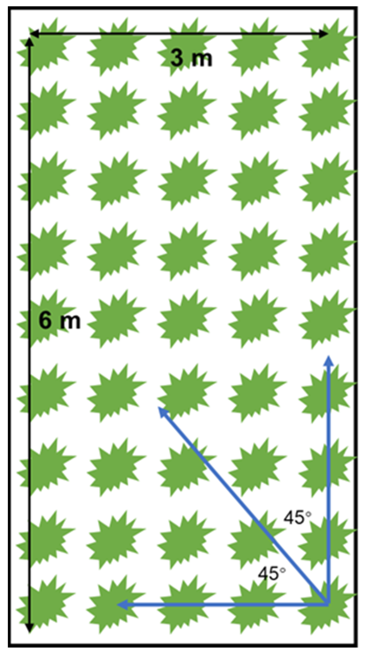
2.1. Study Area

The study area was located in the experimental base of Dryland Agriculture Research Institute of Hebei Academy of Agriculture and Forestry Sciences in Shenzhou City (SZ). The coordinates of the site are 37°54′15.63′′N, 115°42′29.32′′E. It is located in a warm temperate semi-arid region with monsoon climate. It has distinct continental climate characteristics, with distinct seasons and simultaneous occurrence of rain and heat. The average annual temperature is 13.4 °C, and the annual precipitation is 486 mm, which is suitable for the growth of grain crops. The soil in this area is light loam, which is rich in mineral nutrients but deficient in organic matter and available nitrogen and phosphorus nutrients. In addition, Zhoukou City (ZK) in the southern part of North China Plain and Huaibei City (HB) in the eastern part were used to verify the applicability of the selected vegetation indices in different regions. ZK is located at 33°03′–34°20′N and 114°05′–115°39′E, with a total area of about 11,959 square kilometers, and is one of the major grain production bases in the country. HB is located at 116°24′–117°03′E and 33°16′–34°10′N, with an average annual precipitation of 760 mm to 840 mm. At the same time, both regions were subjected to multiple artificial irrigations during the winter wheat growing season, and the growth conditions of winter wheat differed significantly from SZ.

The experiment was conducted in a split-plot model in a randomized complete block design in 2023, with three blocks. The field plots received the different levels of irrigation (IS—

Table 1. Irrigation time and amount of irrigation for the irrigation schemes in the experiment.

Irrigation Scheme	Irrigation Data	Phenological Phase	Total Irrigation Volume (m3 ha−1)
IS-A	2 April 2023	Jointing Flowering	1500
IS-B	None	None	0
IS-C	28 November 2022	Overwintering	750
IS-D	7 March 2023	Regreen	750
IS-E	2 April 2023	Jointing	750
IS-F	9 April 2023	Jointing	750
IS-G	16 April 2023	Booting	750

), and 11 common winter wheat varieties in the North China Plain were distributed in the subplots: T1 (Chang8744), T2 (Shimai22), T3 (Luyuan472), T4 (Shimai15), T5 (HengH1603), T6 (Xinmai28), T7 (Jimai418), T8 (Shannong28), T9 (Nongda212), T10 (Heng4399), and T11 (Jimai22).

Therefore, a total of 231 ground plots were set up, with each plot measuring 1.5 × 6 m, with an area of 9 square meters per plot, and 11 winter wheat varieties were randomly planted in these plots. The distribution of all plots and the distribution of each variety observed for each IS from left to right are shown in Figure 1.

The winter wheat seeds in all plots were sown on 15 October 2022, at a planting density of 375 plants per square meter. The basal fertilizer applied during sowing consisted of pure nitrogen fertilizer (225 kg ha⁻¹), P₂O₅ (112.5 kg ha⁻¹), and K₂O (112.5 kg ha⁻¹). No additional fertilizer was applied during the growing season.

2.2. Ground Data Collection

2.2.1. $f\mathrm{P}\mathrm{A}\mathrm{R}$ Data

$f\mathrm{P}\mathrm{A}\mathrm{R}$ was measured by the SunScan plant canopy analyzer (Produced by Delta-T in the UK), which consists of a 1 m probe and a handheld PDA. The probe contains a total of 64 quantum sensors and is connected to the PDA using an RS-232 cable. When measuring the $f\mathrm{P}\mathrm{A}\mathrm{R}$ of each plot, the incident light and effective radiation were measured separately for 3 canopy incident (${\mathrm{P}\mathrm{A}\mathrm{R}}_{\mathrm{i}\mathrm{n}-\mathrm{c}\mathrm{a}\mathrm{n}}$), 3 canopy reflectance (${\mathrm{P}\mathrm{A}\mathrm{R}}_{\mathrm{r}\mathrm{e}-\mathrm{c}\mathrm{a}\mathrm{n}}$), 3 soil incident (${\mathrm{P}\mathrm{A}\mathrm{R}}_{\mathrm{i}\mathrm{n}-\mathrm{s}\mathrm{o}\mathrm{i}\mathrm{l}}$), and 3 soil reflectance measurements (${\mathrm{P}\mathrm{A}\mathrm{R}}_{\mathrm{r}\mathrm{e}-\mathrm{s}\mathrm{o}\mathrm{i}\mathrm{l}}$) of photosynthetically active radiation (PAR). The $f\mathrm{P}\mathrm{A}\mathrm{R}$ of the plot was obtained by averaging these three measurements. The spatial relationship between the probe and the winter wheat plots is shown in Figure 2. Due to the time-consuming nature of $f\mathrm{P}\mathrm{A}\mathrm{R}$ observations, to ensure that all measurements were completed between 10 a.m. and 2 p.m., only one replicate experiment for each water treatment was selected for ground data collection, resulting in a total of 77 ground plot measurements per session. The horizontal angle between adjacent measurements was set to 45°. The $f\mathrm{P}\mathrm{A}\mathrm{R}$ of each plot is defined as:

$$f\mathrm{P}\mathrm{A}\mathrm{R}=\frac{{\mathrm{P}\mathrm{A}\mathrm{R}}_{\mathrm{i}\mathrm{n}-\mathrm{c}\mathrm{a}\mathrm{n}}-{\mathrm{P}\mathrm{A}\mathrm{R}}_{\mathrm{r}\mathrm{e}-\mathrm{c}\mathrm{a}\mathrm{n}}-\left({\mathrm{P}\mathrm{A}\mathrm{R}}_{\mathrm{i}\mathrm{n}-\mathrm{s}\mathrm{o}\mathrm{i}\mathrm{l}}-{\mathrm{P}\mathrm{A}\mathrm{R}}_{\mathrm{r}\mathrm{e}-\mathrm{s}\mathrm{o}\mathrm{i}\mathrm{l}}\right)}{{\mathrm{P}\mathrm{A}\mathrm{R}}_{\mathrm{i}\mathrm{n}-\mathrm{c}\mathrm{a}\mathrm{n}}}$$

(1)

2.2.2. Spectral Reflectance Data

Winter wheat canopy hyperspectral data were collected using a spectroradiometer (Field Spec 4, wavelength range: 350–2500 nm, spectral resolution: 1 nm) manufactured by ASD (Analytical Spectral Devices Inc., Boulder, CO, USA). The measurements were carried out between 10.00 and 14.00 in good weather conditions and with sufficient illumination. A whiteboard was used for reflectance calibration. The measurement position was approximately 0.5 m from the wheat canopy. At the same position as the $f\mathrm{P}\mathrm{A}\mathrm{R}$ measurement, 10 canopy spectral curves were obtained and their average was taken as the spectral reflectance curve of the plot. The near-ground hyperspectral data were then fitted to the reflectance of different bands from the Sentinel-2 satellite using the spectral response function [34].

The date 28 March represents the early tillering stage for winter wheat, 28 April is the end of tillering and the start of grain filling, and 2 May is the early grain filling stage for winter wheat. The total ground base measurements were performed at two complete phenological stages of tillering and heading, but also early grain filling data, covering the main growth phenophases of winter wheat. The dates and weather conditions of ground data collection are shown in

Table 2. Dates of reflectance and $f\mathrm{P}\mathrm{A}\mathrm{R}$ measurements and the weather conditions.

Date	28 March	30 March	1 April	8 April	11 April	13 April	15 April	18 April	27 April	29 April	2 May
$f\mathrm{P}\mathrm{A}\mathrm{R}$	√	√	√	√	√	√	√	√	√	√	√
Reflec.	√	√	√	√	√	√	√	√	√	√	√
Weather 1	C	C/S	S	S/R	S	C	C	C	C/S	S	C/R

¹ C represents cloudy, S represents sunny, R represents rain, / indicates weather changes, such as S/R indicating sunny to rainy.

.

2.3. Sentinel-2 Data

Sentinel-2 data were used in this study. These data provide high spatial resolution surface reflectance products in 13 bands with a revisit period of approximately 5 days (twin satellites) and a spatial resolution ranging from 10 m to 60 m. They have high application value in agricultural monitoring. Sentinel-2 data at the L2A level, obtained from the Copernicus Data Open Access Hub (https://scihub.copernicus.eu/dhus/#/home (accessed on 15 January 2020)), were used in this study. Vegetation indices were calculated using SNAP 9.0.0 software, and the Biophysical Processor tool was used to calculate $f\mathrm{P}\mathrm{A}\mathrm{R}$ in the field area and to analyze the relationship between satellite winter wheat vegetation indices and $f\mathrm{P}\mathrm{A}\mathrm{R}$. This tool relies mainly on radiative transfer models to generate a comprehensive database of vegetation characteristics and reflectance and then trains a neural network to estimate canopy characteristics from reflectance, providing canopy data with a maximum spatial resolution of 10 m, such as LAI, $f\mathrm{P}\mathrm{A}\mathrm{R}$ and fraction vegetation coverage (FVC).

In this study, Sentinel-2 L2A data were downloaded from early March to late May in SZ. A total of 90 winter wheat plots were obtained by combining high-resolution Google Earth images. Among them, 60 plots were used as training samples and 30 plots as validation samples. These training samples are randomly and uniformly distributed within the selected spatial region of the experimental area. Based on a 100-tree random forest classifier, winter wheat mapping was performed with an overall classification accuracy of 96%. The obtained spatial distribution data of winter wheat were used to mask vegetation indices and $f\mathrm{P}\mathrm{A}\mathrm{R}$ to verify the correlation between satellite vegetation indices and $f\mathrm{P}\mathrm{A}\mathrm{R}$ during key phenological periods.

In order to verify the applicability of the selected vegetation indices in other regions of the North China Plain, the same processing method was used to select winter wheat areas in ZK and HB, and the $f\mathrm{P}\mathrm{A}\mathrm{R}$ values based on the physical model were used to verify the applicability of the $f\mathrm{P}\mathrm{A}\mathrm{R}$ values obtained based on vegetation indices in different regions.

Due to the different bandwidths between the high-spectral data measured by the ASD spectrometer and the Sentinel-2 data, in order to simultaneously compare the applicability of different vegetation indices at different scales, it is necessary to use the satellite’s spectral response function to convert ground spectral data into satellite band reflectance. The method [23] was referenced to establish a one-to-one correspondence between ground reflectance and satellite reflectance. Sentinel 2 data were acquired simultaneously from two satellites, A and B, but there is a certain difference in the central wavelengths of the two satellites (https://sentiwiki.copernicus.eu/web/s2-mission#Acquisition-Resolutions (accessed on 15 January 2020)). In order to facilitate the simulation of ASD data as the reflection of Sentinel 2 data, we have compromised the central wavelengths of the two satellites. For example, the central wavelength of the blue band for Sentinel 2a was 492.7 nm, while was 492.3 for Sentinel 2b. Therefore, we chose 492.5 nm as the center wavelength for the simulation and performed similar processing on other bands. The correspondence between the ASD spectrometer and the satellite is shown in Appendix B.

2.4. Vegetation Indices

A total of 21 common vegetation indices were used to analyze their correlation with ground measured $f\mathrm{P}\mathrm{A}\mathrm{R}$. These vegetation indices have been used to estimate $f\mathrm{P}\mathrm{A}\mathrm{R}$ for different vegetation types and have shown varying degrees of estimation capability. Therefore, the aim of this study is to evaluate their ability to estimate $f\mathrm{P}\mathrm{A}\mathrm{R}$ during the main growth stages of winter wheat. Their definitions and calculation methods are shown in

Table 3. The different vegetation indices used in this study and their calculation methods based on the reflectance bands of the Sentinel 2 data.

Index Name	Definition of Indices 1	Index Name	Definition of Indices 1
NDVI	$\frac{\mathrm{B}8 - \mathrm{B}4}{\mathrm{B}8 + \mathrm{B}4}$	MNDVI	$\frac{0.5 \times \mathrm{B}8 - \mathrm{B}4}{0.5 \times \mathrm{B}8 + \mathrm{B}4}$
EVI	$2.5 \times \frac{\mathrm{B}8 - \mathrm{B}4}{\mathrm{B}8 + 6 \times \mathrm{B}4 - 7.5 \times \mathrm{B}2 + 1}$	SAVI	$\frac{1.5 \times (\mathrm{B}8 - \mathrm{B}4)}{\mathrm{B}8 + \mathrm{B}4 + 0.5}$
EVI2	$2.5 \times \frac{\mathrm{B}8 - \mathrm{B}4}{\mathrm{B}8 + 2.4 \times \mathrm{B}4 + 1}$	OSAVI	$\frac{\mathrm{B}8 - \mathrm{B}4}{\mathrm{B}8 + \mathrm{B}4 + 0.16}$
NDPI	$\frac{\mathrm{B}8 - (0.74 \times \mathrm{B}4 + 0.26 \times \mathrm{B}12)}{\mathrm{B}8 + (0.74 \times \mathrm{B}4 + 0.26 \times \mathrm{B}12)}$	CIG	$\frac{\mathrm{B}7}{\mathrm{B}3} - 1$
GCVI	$\frac{\mathrm{B}8}{\mathrm{B}3} - 1$	CIR	$\frac{\mathrm{B}7}{\mathrm{B}5} - 1$
RVI	$\frac{\mathrm{B}8}{\mathrm{B}4}$	MNDWI	$\frac{\mathrm{B}3 - \mathrm{B}11}{\mathrm{B}3 + \mathrm{B}11}$
DVI	$\mathrm{B}8 - \mathrm{B}4$	NDBI	$\frac{\mathrm{B}8 - \mathrm{B}11}{\mathrm{B}8 + \mathrm{B}11}$
LSWI-b8b11	$\frac{\mathrm{B}8 - \mathrm{B}11}{\mathrm{B}8 + \mathrm{B}11}$	GNDVI	$\frac{\mathrm{B}8 - \mathrm{B}3}{\mathrm{B}8 + \mathrm{B}3}$
LSWI-b8b12	$\frac{\mathrm{B}8 - \mathrm{B}12}{\mathrm{B}8 + \mathrm{B}12}$	NIRV	$\frac{\mathrm{B}8 - \mathrm{B}4}{\mathrm{B}8 + \mathrm{B}4} \times \mathrm{B}8$
LSWI-b8Ab11	$\frac{\mathrm{B}8\mathrm{A} - \mathrm{B}11}{\mathrm{B}8\mathrm{A} + \mathrm{B}11}$	MTCI	$\frac{\mathrm{B}6 - \mathrm{B}5}{\mathrm{B}5 - \mathrm{B}4}$
LSWI-b8Ab12	$\frac{\mathrm{B}8\mathrm{A}-\mathrm{B}12}{\mathrm{B}8\mathrm{A} + \mathrm{B}12}$

¹ In the equation, B4, B8, and others are the band numbers of the simulated Sentinel 2 data in Table A2.

.

The correlation between vegetation indices and $f\mathrm{P}\mathrm{A}\mathrm{R}$ is typically represented by linear, power, and exponential functions. We simulated the ground-based ASD reflectance data as Sentinel-2 vegetation indices and established three different estimation models: linear, exponential, and logarithmic. We then selected the most stable vegetation index in terms of correlation during key growth stages and validated its accuracy at the satellite scale using Sentinel-2 data.

2.5. Accuracy Assessment

Due to the effect of low temperatures, the emergence rate of the T3 and T5 varieties under certain irrigation conditions was insufficient, resulting in poor growth of the whole winter wheat plot. In addition, the emergence rate of some varieties under different irrigation conditions did not meet the measurement standards. Therefore, plot data with $f\mathrm{P}\mathrm{A}\mathrm{R}$ measurements below 0 were excluded during modeling and validation. The coefficient of determination (Equation (2)) and root mean squared error (RMSE—Equation (3)) were used to assess the stability and accuracy of the correlation relationships:

$${\mathrm{R}}^2=\frac{{\sum }_i^n{\left(\widehat{{f\mathrm{P}\mathrm{A}\mathrm{R}}_i}-\overline{{f\mathrm{P}\mathrm{A}\mathrm{R}}_i}\right)}^2}{{\sum }_i^n{\left({f\mathrm{P}\mathrm{A}\mathrm{R}}_i-\overline{{f\mathrm{P}\mathrm{A}\mathrm{R}}_i}\right)}^2},$$

(2)

$$\mathrm{R}\mathrm{M}\mathrm{S}\mathrm{E}=\sqrt{\frac{1}{n}{\sum }_{i=0}^n{\left({f\mathrm{P}\mathrm{A}\mathrm{R}}_i-\widehat{{f\mathrm{P}\mathrm{A}\mathrm{R}}_i}\right)}^2},$$

(3)

where ${f\mathrm{P}\mathrm{A}\mathrm{R}}_i$ represents the actual ground measurement value, $\widehat{{f\mathrm{P}\mathrm{A}\mathrm{R}}_i}$ represents the estimated value of the model, and $\overline{{f\mathrm{P}\mathrm{A}\mathrm{R}}_i}$ represents the mean value of the estimates, $n$ represents the number of plots participating in the accuracy validation, and $i$ represents the $i$-th ground plot. The statistical tool used in this study is based on R language code to fit the correlation between $f\mathrm{P}\mathrm{A}\mathrm{R}$ and different vegetation indices. At the same time, the coefficient of determination ${\mathrm{R}}^2$ and the root mean square error (RMSE) of the model are calculated and plotted in Excel.

3. Results

3.1. Correlation between Vegetation Indices at Different Phenological Stages

Different weather conditions exist on different observation dates, and due to seasonal changes, variations in the solar zenith angle may cause changes in the correlation between vegetation indices and $f\mathrm{P}\mathrm{A}\mathrm{R}$ on different measurement dates. In this study, the near-ground reflectance of all 11 measurement days is simulated as Sentinel-2 vegetation indices, and three estimation models (linear, exponential, and logarithmic) were established with $f\mathrm{P}\mathrm{A}\mathrm{R}$ measured by SunScan. The coefficient of determination ${\mathrm{R}}^2$ was also calculated. The results of linear correlation are shown in

Table 4. Determination coefficient ${\mathrm{R}}^2$ of linear correlation between vegetation indices and fPAR.

Date	28 March	30 March	1 April	8 April	11 April	13 April	15 April	18 April	27 April	29 April	2 May
NDPI	0.583	0.659	0.621	0.719	0.621	0.742	0.812	0.828	0.324	0.550	0.919
NDVI	0.588	0.643	0.685	0.721	0.612	0.758	0.821	0.839	0.500	0.681	0.917
MNDVI	0.596	0.674	0.695	0.732	0.652	0.761	0.830	0.840	0.498	0.679	0.911
LSWIB8B12	0.523	0.607	0.442	0.616	0.567	0.632	0.733	0.760	0.183	0.364	0.899
LSWIB8aB12	0.520	0.607	0.439	0.615	0.567	0.630	0.729	0.758	0.180	0.365	0.899
OSAVI	0.672	0.648	0.725	0.741	0.636	0.717	0.835	0.812	0.570	0.740	0.897
NDWI	0.506	0.602	0.565	0.728	0.622	0.640	0.817	0.809	0.375	0.516	0.882
LSWIB8B11	0.541	0.658	0.438	0.632	0.572	0.630	0.720	0.756	0.160	0.371	0.878
NDBI	0.541	0.658	0.438	0.632	0.572	0.630	0.720	0.756	0.160	0.371	0.878
LSWIB8aB11	0.536	0.658	0.434	0.629	0.570	0.627	0.714	0.753	0.155	0.372	0.877
SAVI	0.715	0.646	0.705	0.703	0.622	0.630	0.799	0.726	0.431	0.661	0.837
EVI2	0.725	0.655	0.698	0.687	0.626	0.612	0.785	0.699	0.412	0.640	0.808
EVI	0.720	0.652	0.659	0.639	0.605	0.560	0.770	0.674	0.316	0.573	0.779
NIRV	0.731	0.644	0.640	0.634	0.582	0.536	0.726	0.611	0.357	0.588	0.742
DVI	0.712	0.616	0.565	0.589	0.526	0.466	0.675	0.543	0.314	0.541	0.683
CIG	0.501	0.545	0.486	0.600	0.589	0.597	0.772	0.701	0.321	0.432	0.639
CIR	0.590	0.632	0.616	0.580	0.617	0.670	0.767	0.664	0.421	0.556	0.636
GCVI	0.492	0.541	0.481	0.594	0.582	0.594	0.769	0.695	0.321	0.432	0.631
RVI	0.585	0.631	0.614	0.577	0.614	0.669	0.767	0.660	0.422	0.556	0.631
MNDWI	0.150	0.307	0.237	0.574	0.536	0.146	0.418	0.679	0.261	0.318	0.238
MTCI	0.550	0.502	0.497	0.646	0.587	0.617	0.661	0.573	0.437	0.354	0.361

.

In terms of linear correlation, MNDVI is the most stable. In the 11 measurement results, the correlation coefficient was in the top five for all vegetation indices ten times. NDVI and OSAVI followed with a total of eight occurrences, and NDPI had six occurrences within the top five. This indicates that MNDVI can achieve a high level of estimation capability for $f\mathrm{P}\mathrm{A}\mathrm{R}$ under different light conditions throughout the critical growth period. The results of the exponential correlation are shown in

Table 5. Determination coefficient ${\mathrm{R}}^2$ of exponential correlation between vegetation indices and fPAR.

Date	28 March	30 March	1 April	8 April	11 April	13 April	15 April	18 April	27 April	29 April	2 May
NDVI	0.667	0.686	0.719	0.766	0.794	0.755	0.814	0.777	0.510	0.704	0.912
NDPI	0.640	0.655	0.642	0.731	0.775	0.720	0.792	0.765	0.336	0.569	0.887
MNDVI	0.668	0.686	0.721	0.765	0.804	0.753	0.817	0.775	0.506	0.699	0.885
OSAVI	0.732	0.661	0.750	0.769	0.789	0.711	0.816	0.755	0.550	0.748	0.867
LSWIB8B12	0.571	0.564	0.453	0.616	0.724	0.610	0.710	0.705	0.196	0.385	0.861
LSWIB8aB12	0.560	0.563	0.449	0.614	0.724	0.607	0.706	0.703	0.193	0.386	0.861
NDWI	0.542	0.492	0.571	0.714	0.770	0.616	0.790	0.750	0.379	0.520	0.854
LSWIB8B11	0.573	0.563	0.442	0.599	0.668	0.593	0.681	0.696	0.171	0.384	0.807
NDBI	0.563	0.563	0.442	0.599	0.668	0.593	0.681	0.696	0.171	0.384	0.807
LSWIB8aB11	0.559	0.561	0.437	0.596	0.665	0.590	0.676	0.692	0.166	0.384	0.806
SAVI	0.751	0.618	0.718	0.713	0.737	0.622	0.769	0.675	0.407	0.658	0.788
EVI2	0.750	0.605	0.703	0.683	0.711	0.601	0.748	0.646	0.386	0.633	0.747
EVI	0.745	0.596	0.671	0.648	0.700	0.558	0.739	0.625	0.293	0.571	0.733
NIRV	0.734	0.559	0.628	0.614	0.624	0.524	0.678	0.561	0.332	0.575	0.669
DVI	0.704	0.514	0.558	0.572	0.568	0.456	0.631	0.501	0.291	0.528	0.614
CIG	0.493	0.410	0.448	0.485	0.550	0.544	0.701	0.619	0.314	0.414	0.531
GCVI	0.484	0.406	0.443	0.512	0.542	0.541	0.697	0.614	0.313	0.413	0.522
CIR	0.568	0.549	0.554	0.492	0.536	0.605	0.686	0.570	0.411	0.531	0.505
RVI	0.564	0.548	0.552	0.490	0.532	0.603	0.686	0.567	0.411	0.530	0.499
MNDWI	0.165	0.137	0.223	0.537	0.556	0.143	0.404	0.612	0.234	0.284	0.235
MTCI	0.571	0.462	0.473	0.602	0.602	0.601	0.570	0.541	0.502	0.344	0.348

.

In the exponential correlation between $f\mathrm{P}\mathrm{A}\mathrm{R}$ and vegetation indices, OSAVI is the most stable. On all eleven observation dates, the coefficient of determination is in the top five for all vegetation indices. NDVI and MNDVI follow with ten occurrences each, while NDPI appears in the top five eight times. The results of the logarithmic correlation are shown in

Table 6. Determination coefficient ${\mathrm{R}}^2$ of logarithmic correlation between vegetation indices and fPAR.

Date	28 March	30 March	1 April	8 April	11 April	13 April	15 April	18 April	27 April	29 April	2 May
LSWIB8aB12	0.509	0.498	0.434	0.604	0.522	0.627	0.730	0.767	0.177	0.358	0.970
NDPI	0.568	0.563	0.611	0.704	0.578	0.737	0.810	0.838	0.321	0.543	0.897
NDVI	0.574	0.568	0.674	0.704	0.573	0.752	0.814	0.847	0.498	0.674	0.891
OSAVI	0.657	0.551	0.713	0.724	0.599	0.711	0.833	0.822	0.572	0.733	0.882
LSWIB8B12	0.511	0.498	0.437	0.606	0.521	0.629	0.739	0.769	0.181	0.357	0.869
LSWIB8aB11	0.519	0.513	0.426	0.619	0.506	0.626	0.724	0.768	0.152	0.362	0.859
LSWIB8B11	0.522	0.515	0.431	0.621	0.502	0.629	0.729	0.772	0.156	0.361	0.858
MNDVI	0.568	0.560	0.672	0.698	0.559	0.749	0.817	0.855	0.494	0.666	0.848
SAVI	0.702	0.519	0.695	0.688	0.589	0.624	0.802	0.737	0.436	0.655	0.832
EVI2	0.711	0.513	0.689	0.672	0.591	0.606	0.793	0.713	0.417	0.636	0.809
EVI	0.706	0.488	0.648	0.623	0.570	0.553	0.775	0.687	0.321	0.568	0.774
NIRV	0.718	0.476	0.632	0.622	0.551	0.530	0.744	0.630	0.366	0.586	0.752
CIR	0.542	0.547	0.629	0.592	0.599	0.668	0.838	0.768	0.417	0.565	0.725
RVI	0.548	0.552	0.628	0.593	0.602	0.670	0.840	0.761	0.420	0.566	0.719
DVI	0.705	0.439	0.561	0.582	0.506	0.461	0.692	0.556	0.322	0.541	0.693
CIG	0.474	0.409	0.491	0.609	0.568	0.601	0.820	0.756	0.320	0.440	0.688
GCVI	0.466	0.407	0.487	0.604	0.562	0.599	0.818	0.749	0.321	0.440	0.682
MTCI	0.533	0.507	0.495	0.634	0.566	0.608	0.672	0.580	0.414	0.346	0.359

.

In logarithmic correlation, OSAVI still performs the best, followed by NDVI and NDPI. However, the coefficient of determination ${\mathrm{R}}^2$ is lower compared to linear and exponential correlations.

Through the analysis of these three correlations, the correlation results are consistent with Dong [33], indicating the reliability of our observational accuracy. The differences in the correlations indicate that variations in weather conditions, water stress levels, and crop varieties during the observation period led to different correlation relationships. It is difficult to establish different correlation models for different growth stages, varieties, lighting conditions, and water stress during the actual estimation process. In addition, it is difficult to obtain irrigation and variety data for winter wheat in the North China Plain. Therefore, using a single vegetation index to establish a stable and highly correlated model is more feasible and convenient in practical production and life.

3.2. Comparison of the Estimation Ability of Vegetation Index for fPAR at the Entire Crop Season

In Section 3.1, we found that the correlation between vegetation indices and $f\mathrm{P}\mathrm{A}\mathrm{R}$ is strongly influenced by external factors. In order to find a more stable and strongly correlated vegetation index, this study simulated the near-surface reflectance of all 11 days as Sentinel-2 vegetation indices and established three correlation relationships with $f\mathrm{P}\mathrm{A}\mathrm{R}$ measured by SunScan. The coefficient of determination ${\mathrm{R}}^2$ was calculated and the root mean square error (RMSE) was calculated using all measurement data for validation. The results are compared in

Table 7. Statistical parameters of linear, exponential, and logarithmic estimation models between $f\mathrm{P}\mathrm{A}\mathrm{R}$ and vegetation indices across the entire crop season.

VI Name	Correlation	Equation	${\mathbf{R}}^2$	RMSE
NDVI	Linear	$fPAR=2.0245VI-1.0714$	0.5926	0.1460
	Exponential	$f\mathrm{P}\mathrm{A}\mathrm{R}={0.0135\mathrm{e}}^{4.416\mathrm{V}\mathrm{I}}$	0.6639	0.1350
	Logarithmic	$f\mathrm{P}\mathrm{A}\mathrm{R}=0.897+1.4085\ln \left(\mathrm{V}\mathrm{I}\right)$	0.5350	0.1479
EVI	Linear	$f\mathrm{P}\mathrm{A}\mathrm{R}=0.8841\mathrm{V}\mathrm{I}-0.0778$	0.3183	0.1896
	Exponential	$f\mathrm{P}\mathrm{A}\mathrm{R}={0.1137\mathrm{e}}^{1.9701\mathrm{V}\mathrm{I}}$	0.2793	0.2039
	Logarithmic	$f\mathrm{P}\mathrm{A}\mathrm{R}=0.7987+0.6834\ln \left(\mathrm{V}\mathrm{I}\right)$	0.3312	0.1812
EVI2	Linear	$f\mathrm{P}\mathrm{A}\mathrm{R}=1.0278\mathrm{V}\mathrm{I}-0.1327$	0.3710	0.1878
	Exponential	$f\mathrm{P}\mathrm{A}\mathrm{R}={0.1047\mathrm{e}}^{2.2415\mathrm{V}\mathrm{I}}$	0.3271	0.1976
	Logarithmic	$f\mathrm{P}\mathrm{A}\mathrm{R}=0.8652+0.7263\ln \left(\mathrm{V}\mathrm{I}\right)$	0.3795	01810
NDPI	Linear	$f\mathrm{P}\mathrm{A}\mathrm{R}=1.9513\mathrm{V}\mathrm{I}-0.7944$	0.6174	0.1314
	Exponential	$f\mathrm{P}\mathrm{A}\mathrm{R}=0.0262{\mathrm{e}}^{4.178\mathrm{V}\mathrm{I}}$	0.5993	0.1379
	Logarithmic	$f\mathrm{P}\mathrm{A}\mathrm{R}=1.0248+1.1763\ln \left(\mathrm{V}\mathrm{I}\right)$	0.5595	0.1418
GCVI	Linear	$f\mathrm{P}\mathrm{A}\mathrm{R}=0.0537\mathrm{V}\mathrm{I}+0.2337$	0.5601	0.1513
	Exponential	$f\mathrm{P}\mathrm{A}\mathrm{R}={0.2605\mathrm{e}}^{0.1041\mathrm{V}\mathrm{I}}$	0.4554	0.1846
	Logarithmic	$f\mathrm{P}\mathrm{A}\mathrm{R}=-0.1525+0.4101\ln \left(\mathrm{V}\mathrm{I}\right)$	0.6191	0.1408
RVI	Linear	$f\mathrm{P}\mathrm{A}\mathrm{R}=0.0189\mathrm{V}\mathrm{I}+0.3206$	0.5625	0.1510
	Exponential	$f\mathrm{P}\mathrm{A}\mathrm{R}={0.3101\mathrm{e}}^{0.0364\mathrm{V}\mathrm{I}}$	0.4403	0.1900
	Logarithmic	$f\mathrm{P}\mathrm{A}\mathrm{R}=-0.2361+0.3266\ln \left(\mathrm{V}\mathrm{I}\right)$	0.6569	0.1342
DVI	Linear Exponential Logarithmic Linear Exponential Logarithmic	$f\mathrm{P}\mathrm{A}\mathrm{R}=0.9682\mathrm{V}\mathrm{I}+0.1724$	0.2292	0.2510
		$f\mathrm{P}\mathrm{A}\mathrm{R}={0.2016\mathrm{e}}^{2.1295\mathrm{V}\mathrm{I}}$	0.2056	0.2608
		$f\mathrm{P}\mathrm{A}\mathrm{R}=1.014+0.4972\ln \left(\mathrm{V}\mathrm{I}\right)$	0.2492	0.2342
LSWI-b8b11		$f\mathrm{P}\mathrm{A}\mathrm{R}=1.5195\mathrm{V}\mathrm{I}-0.4365$	0.4828	0.1643
		$f\mathrm{P}\mathrm{A}\mathrm{R}={0.0561\mathrm{e}}^{3.2612\mathrm{V}\mathrm{I}}$	0.5029	0.1641
		$f\mathrm{P}\mathrm{A}\mathrm{R}=0.9571+0.8496\ln \left(\mathrm{V}\mathrm{I}\right)$	0.4309	0.1722
LSWI-b8b12	Linear	$f\mathrm{P}\mathrm{A}\mathrm{R}=1.6303\mathrm{V}\mathrm{I}-0.5253$	0.5099	0.1598
	Exponential	$f\mathrm{P}\mathrm{A}\mathrm{R}={0.0453\mathrm{e}}^{3.5301\mathrm{V}\mathrm{I}}$	0.5252	0.1704
	Logarithmic	$f\mathrm{P}\mathrm{A}\mathrm{R}=0.9679+0.8994\ln \left(\mathrm{V}\mathrm{I}\right)$	0.4498	0.1698
LSWI-b8Ab11	Linear	$f\mathrm{P}\mathrm{A}\mathrm{R}=1.7019\mathrm{V}\mathrm{I}-0.1852$	0.5899	0.1465
	Exponential	$f\mathrm{P}\mathrm{A}\mathrm{R}={0.1022\mathrm{e}}^{3.5364\mathrm{V}\mathrm{I}}$	0.5437	0.1615
	Logarithmic	$f\mathrm{P}\mathrm{A}\mathrm{R}=1.1191+0.6148\log \left(\mathrm{V}\mathrm{I}\right)$	0.5147	0.1593
LSWI-b8Ab12	Linear	$f\mathrm{P}\mathrm{A}\mathrm{R}=1.6419\mathrm{V}\mathrm{I}-0.5382$	0.5065	0.1603
	Exponential	$f\mathrm{P}\mathrm{A}\mathrm{R}={0.044\mathrm{e}}^{3.5563\mathrm{V}\mathrm{I}}$	0.5718	0.1610
	Logarithmic	$f\mathrm{P}\mathrm{A}\mathrm{R}=0.9693+0.9155\log \left(\mathrm{V}\mathrm{I}\right)$	0.4486	0.1693
MNDVI	Linear	$f\mathrm{P}\mathrm{A}\mathrm{R}=1.2789\mathrm{V}\mathrm{I}-2.853$	0.6184	0.1413
	Exponential	$f\mathrm{P}\mathrm{A}\mathrm{R}={0.0772\mathrm{e}}^{2.7526\mathrm{V}\mathrm{I}}$	0.6649	0.1340
	Logarithmic	$f\mathrm{P}\mathrm{A}\mathrm{R}=0.8524+0.5247\ln \left(\mathrm{V}\mathrm{I}\right)$	0.4507	0.1697
SAVI	Linear	$f\mathrm{P}\mathrm{A}\mathrm{R}=1.4475\mathrm{V}\mathrm{I}-0.3471$	0.3939	0.1789
	Exponential	$f\mathrm{P}\mathrm{A}\mathrm{R}={0.0643\mathrm{e}}^{3.1839\mathrm{V}\mathrm{I}}$	0.3550	0.1921
	Logarithmic	$f\mathrm{P}\mathrm{A}\mathrm{R}=1.0034+0.9054\log \left(\mathrm{V}\mathrm{I}\right)$	0.3926	0.1791
OSAVI	Linear	$f\mathrm{P}\mathrm{A}\mathrm{R}=2.0953\mathrm{V}\mathrm{I}-0.7524$	0.5131	0.1602
	Exponential	$f\mathrm{P}\mathrm{A}\mathrm{R}={0.0267\mathrm{e}}^{4.5933\mathrm{V}\mathrm{I}}$	0.5088	0.1642
	Logarithmic	$f\mathrm{P}\mathrm{A}\mathrm{R}=1.1456+1.1901\ln \left(\mathrm{V}\mathrm{I}\right)$	0.4815	0.1642
CIG	Linear	$f\mathrm{P}\mathrm{A}\mathrm{R}=0.0555\mathrm{V}\mathrm{I}+0.2298$	0.5663	0.1503
	Exponential	$f\mathrm{P}\mathrm{A}\mathrm{R}={0.2583\mathrm{e}}^{0.1078\mathrm{V}\mathrm{I}}$	0.4619	0.1874
	Logarithmic	$f\mathrm{P}\mathrm{A}\mathrm{R}=-0.1415+0.4099\ln \left(\mathrm{V}\mathrm{I}\right)$	0.6229	0.1401
CIR	Linear	$f\mathrm{P}\mathrm{A}\mathrm{R}=0.0194\mathrm{V}\mathrm{I}+0.3379$	0.5652	0.1504
	Exponential	$f\mathrm{P}\mathrm{A}\mathrm{R}={0.3205\mathrm{e}}^{0.0374\mathrm{V}\mathrm{I}}$	0.4432	0.1925
	Logarithmic	$f\mathrm{P}\mathrm{A}\mathrm{R}=-0.1098+0.2925\ln \left(\mathrm{V}\mathrm{I}\right)$	0.6545	0.1346
MNDVI	Linear	$f\mathrm{P}\mathrm{A}\mathrm{R}=-2.0363\mathrm{V}\mathrm{I}-0.2734$	0.3038	0.1908
	Exponential	$\mathrm{f}\mathrm{P}\mathrm{A}\mathrm{R}=0.0939{\mathrm{e}}^{-4.027\mathrm{V}\mathrm{I}}$	0.2924	0.1981
NDBI	Linear	$f\mathrm{P}\mathrm{A}\mathrm{R}=-1.6941\mathrm{V}\mathrm{I}-0.1741$	0.5951	0.1445
	Exponential	$f\mathrm{P}\mathrm{A}\mathrm{R}=0.1047{\mathrm{e}}^{-3.519\mathrm{V}\mathrm{I}}$	0.5490	0.1983
NDWI	Linear	$f\mathrm{P}\mathrm{A}\mathrm{R}=-2.2472\mathrm{V}\mathrm{I}-1.0779$	0.6097	0.1423
	Exponential	$f\mathrm{P}\mathrm{A}\mathrm{R}=0.0155{\mathrm{e}}^{-4.71\mathrm{V}\mathrm{I}}$	0.6166	0.149 3
NIRV	Linear	$f\mathrm{P}\mathrm{A}\mathrm{R}=1.0492\mathrm{V}\mathrm{I}+0.1605$	0.2966	0.1924
	Exponential	$f\mathrm{P}\mathrm{A}\mathrm{R}={0.1998\mathrm{e}}^{2.2752\mathrm{V}\mathrm{I}}$	0.2582	0.2182
	Logarithmic	$f\mathrm{P}\mathrm{A}\mathrm{R}=1.0382+0.4852\ln \left(\mathrm{V}\mathrm{I}\right)$	0.3228	0.1890
MTCI	Linear	$f\mathrm{P}\mathrm{A}\mathrm{R}=0.1447\mathrm{V}\mathrm{I}-0.1454$	0.5749	0.1490
	Exponential	$f\mathrm{P}\mathrm{A}\mathrm{R}=0.1176e^{0.2909VI}$	0.4807	0.1845
	Logarithmic	$f\mathrm{P}\mathrm{A}\mathrm{R}=-0.6513+0.7761\ln \left(\mathrm{V}\mathrm{I}\right)$	0.6001	0.1464

.

Among them, MNDWI, NDBI, and NDWI values are less than 0, so there is no logarithmic correlation with $f\mathrm{P}\mathrm{A}\mathrm{R}$. The fitting results show that different vegetation indices have significant differences in fitting $f\mathrm{P}\mathrm{A}\mathrm{R}$, and the accuracy of linear, exponential, and logarithmic fits also varies. OSAVI shows better estimation ability in discriminating observation dates, but throughout the critical growth period, its coefficient of determination ${\mathrm{R}}^2$ with $f\mathrm{P}\mathrm{A}\mathrm{R}$ is highest at 0.5131. This indicates that OSAVI is strongly influenced by lighting conditions and the correlation model established using it lacks stability, making it difficult to estimate $f\mathrm{P}\mathrm{A}\mathrm{R}$ for the entire critical growth period. When a single vegetation index is used for fitting, MNDVI, NDVI, NDPI, RVI, and DVI show good fitting accuracy. Among them, MNDVI maintains a high correlation both throughout the critical growth period and at different dates, indicating its stability in different phenological stages, different solar weather conditions, and solar zenith angles. Therefore, MNDVI has great potential for the estimation of fPAR.

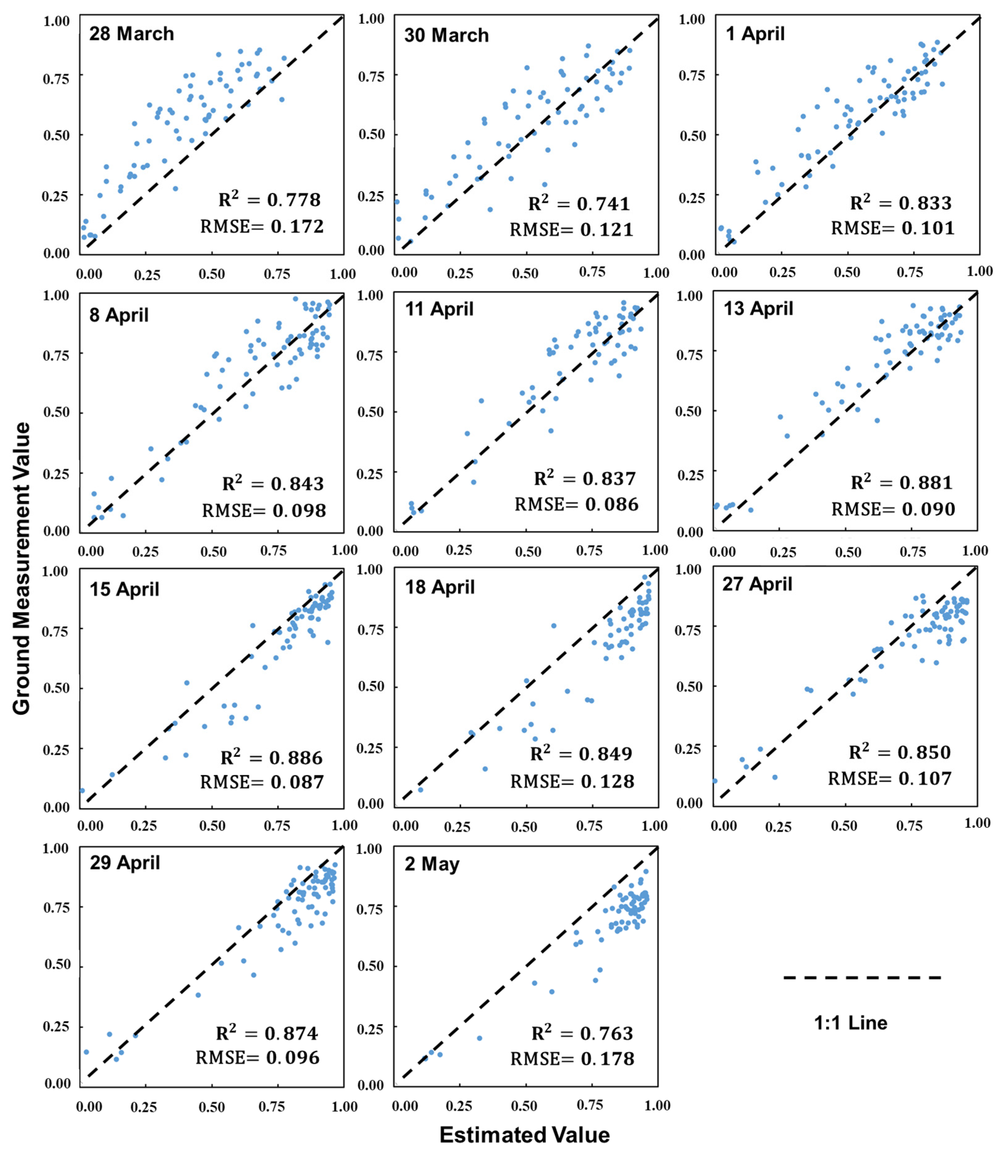
3.3. Stability Test of MNDVI Estimation for fPAR

In Section 3.2, we found that MNDVI has high stability and correlation in estimating $f\mathrm{P}\mathrm{A}\mathrm{R}$ during the entire critical growth period of winter wheat. However, whether using the same correlation equation for $f\mathrm{P}\mathrm{A}\mathrm{R}$ estimation during the critical growth period can maintain high accuracy across different varieties and irrigation schemes still needs to be verified. Therefore, in this study, the estimated values of $f\mathrm{P}\mathrm{A}\mathrm{R}$ were obtained based on the following equation:

$$f\mathrm{P}\mathrm{A}\mathrm{R}={0.0772\mathrm{e}}^{2.7526\mathrm{M}\mathrm{N}\mathrm{D}\mathrm{V}\mathrm{I}},$$

(4)

To verify the accuracy of the estimated values, the study used actual measured values for validation and used the coefficient of determination ${\mathrm{R}}^2$ and the root mean square error RMSE as accuracy evaluation indicators to assess the robustness across different varieties, irrigation schemes, and dates.

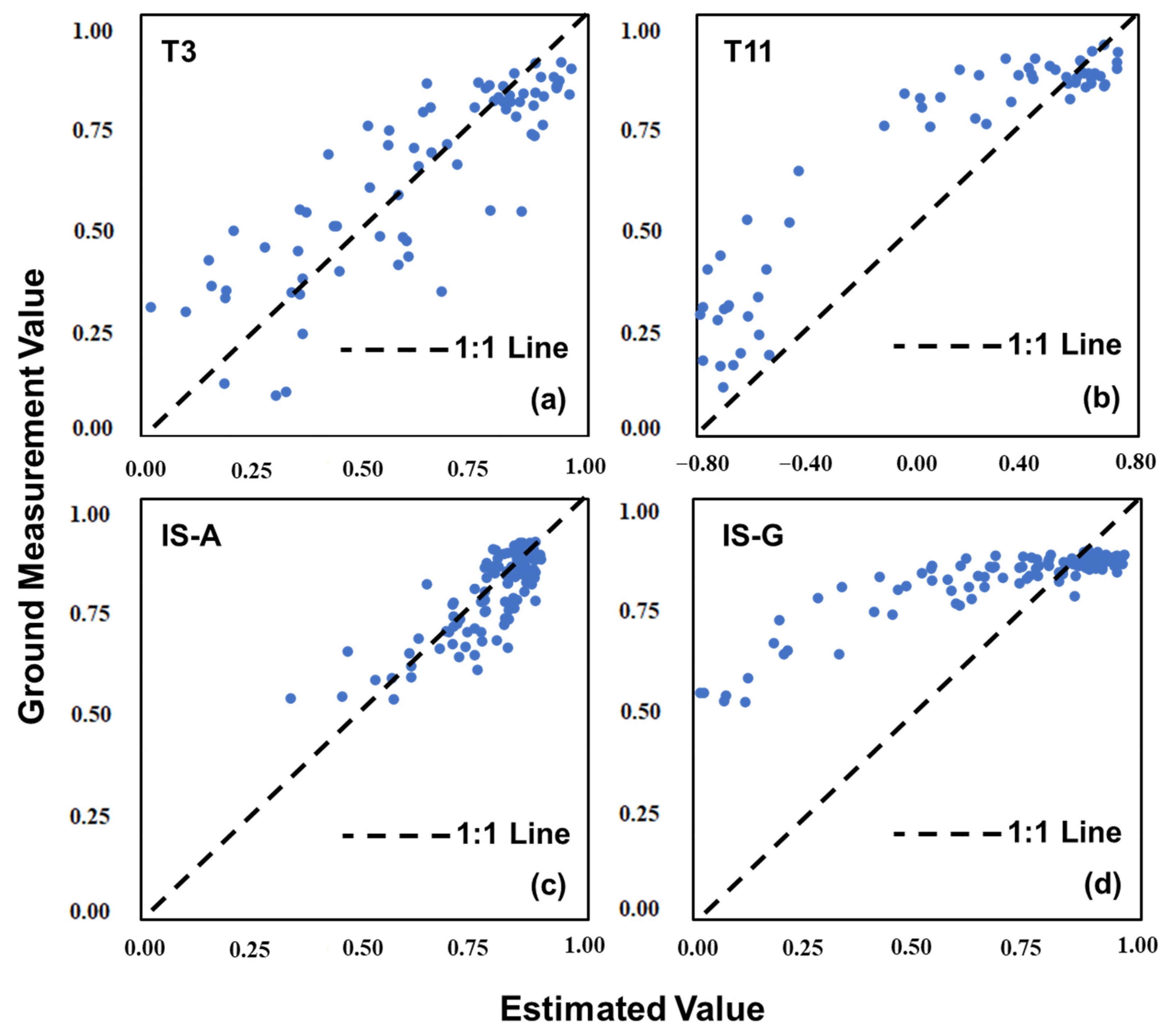
3.3.1. Accuracy Assessment Based on Different Varieties

The measurement of canopy reflectance and $f\mathrm{P}\mathrm{A}\mathrm{R}$ could not be completed due to insufficient emergence of T3 and T5 varieties in some plots and the inability to measure IS-F and IS-G in all plots on 11 April and 18 April due to irrigation. However, the measurements from all other plots were included in the accuracy validation. Figure 3 shows the relationship between the estimated values calculated using Equation (3) and the ground truth measured values, where the horizontal axis represents the estimated values and the vertical axis represents the measured values.

It can be seen that, with the exception of variety T10, the other varieties have a good correlation and a low RMSE. The variety T6 has the highest coefficient of determination of 0.918, while variety T1 has the lowest RMSE of 0.074. This indicates that MNDVI can maintain high stability among different varieties, and in actual production processes in regions such as the North China Plain, it is difficult to obtain extensive sowing data. MNDVI has great potential for application in yield estimation in these research areas.

3.3.2. Accuracy Assessment Based on Different Lighting Conditions

When estimating the vegetation index $f\mathrm{P}\mathrm{A}\mathrm{R}$, the changing light conditions during crop growth, including solar zenith angle and light intensity under different weather conditions, play a crucial role in determining the stability of the correlation between the vegetation index and $f\mathrm{P}\mathrm{A}\mathrm{R}$. These light conditions include solar zenith angle and light intensity under different weather conditions, which can affect the correlation between $f\mathrm{P}\mathrm{A}\mathrm{R}$ and other indicators. Therefore, when using MNDVI to estimate $f\mathrm{P}\mathrm{A}\mathrm{R}$, it is necessary to validate the accuracy of this index on different observation dates. To validate the estimation accuracy of MNDVI on different observation dates, we calculated the corresponding estimated values using Equation (3). These estimates represent the $f\mathrm{P}\mathrm{A}\mathrm{R}$ at different observation dates. Our study aims to demonstrate the high stability of using MNDVI for $f\mathrm{P}\mathrm{A}\mathrm{R}$ estimation during different phenological stages and under varying light conditions. The accuracy validation results are shown in Figure 4, which contributes to evaluating the applicability of this method under different environmental conditions.

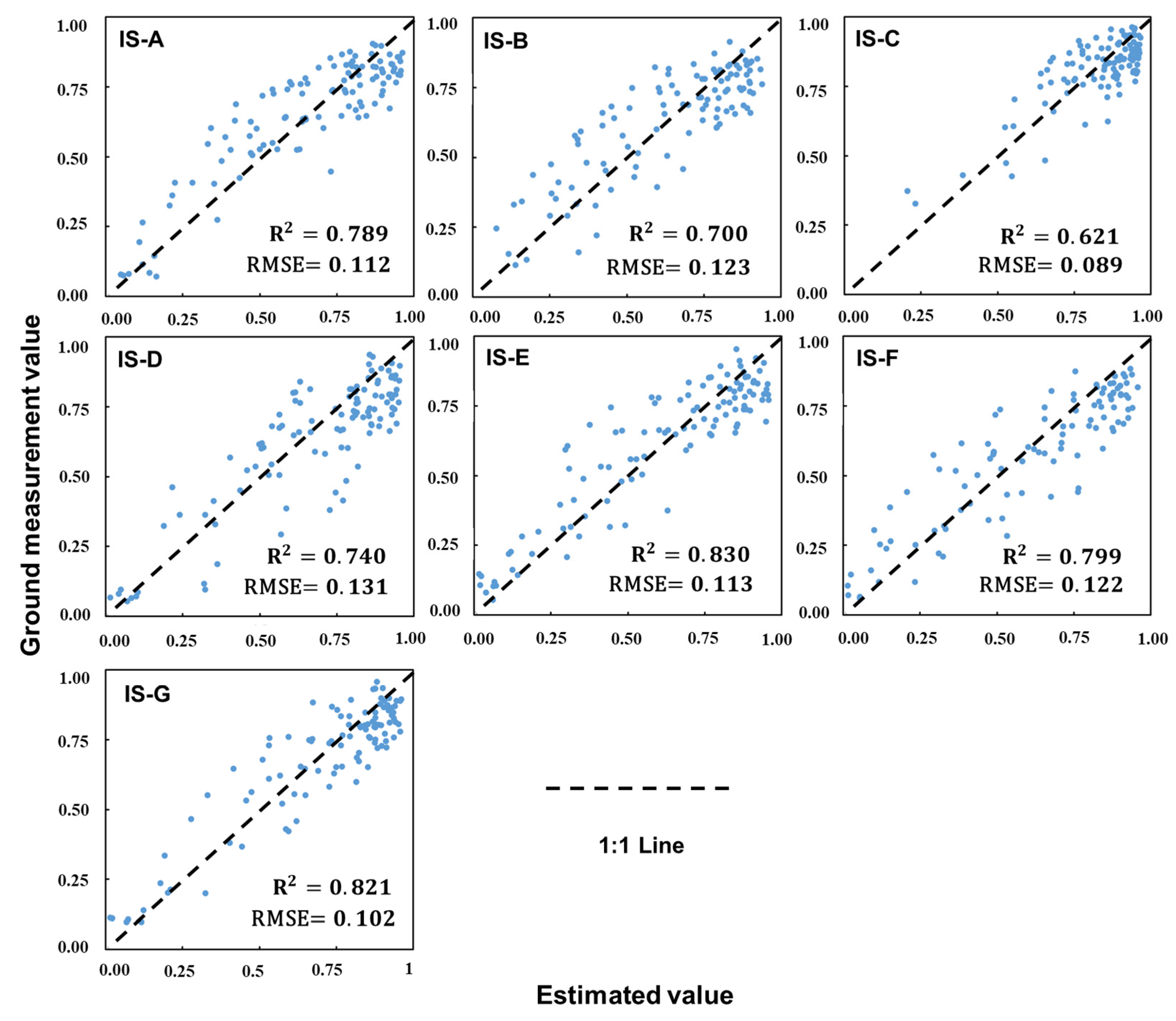
3.3.3. Accuracy Assessment Based on Different Irrigation Scheme

The irrigation scheme has caused varying degrees of water stress on winter wheat, as the North China Plain has a wide spatial range and uneven distribution of precipitation. To validate the stability of estimating $f\mathrm{P}\mathrm{A}\mathrm{R}$ using MNDVI under different water stress-induced growth variations, and to ensure that the estimation accuracy of relevant models is not significantly reduced when applied on a large scale and influenced by crop growth status. The validation results are shown in Figure 5.

Comparing the estimated results with the actual measured results, except for the IS-C irrigation scheme, which has a relatively lower coefficient of determination, the accuracy of the other different water stress levels can generally meet the requirements of practical application. The IS-C scheme has good growth performance in almost all plot areas, which makes it difficult to obtain a high ${\mathrm{R}}^2$, but it has the lowest RMSE. This indicates that MNDVI can consistently and accurately estimate $f\mathrm{P}\mathrm{A}\mathrm{R}$ under different levels of water stress.

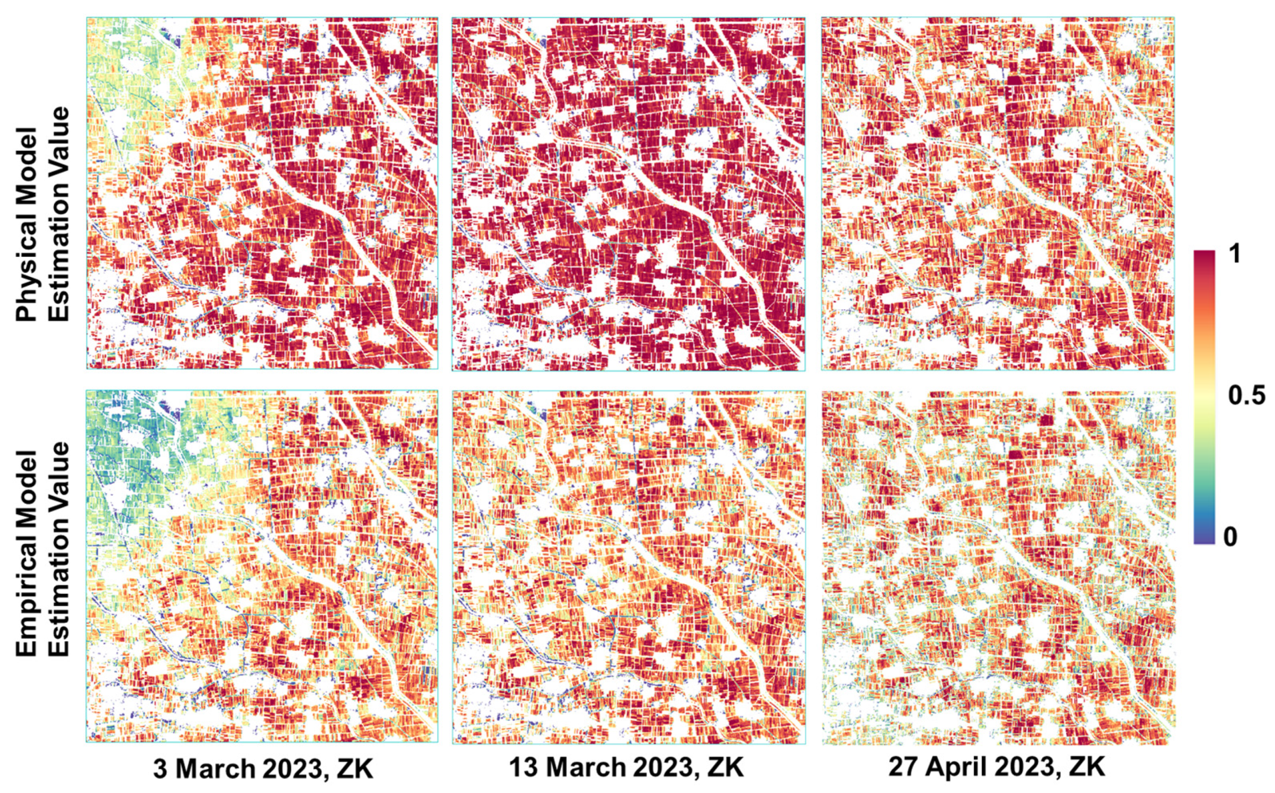
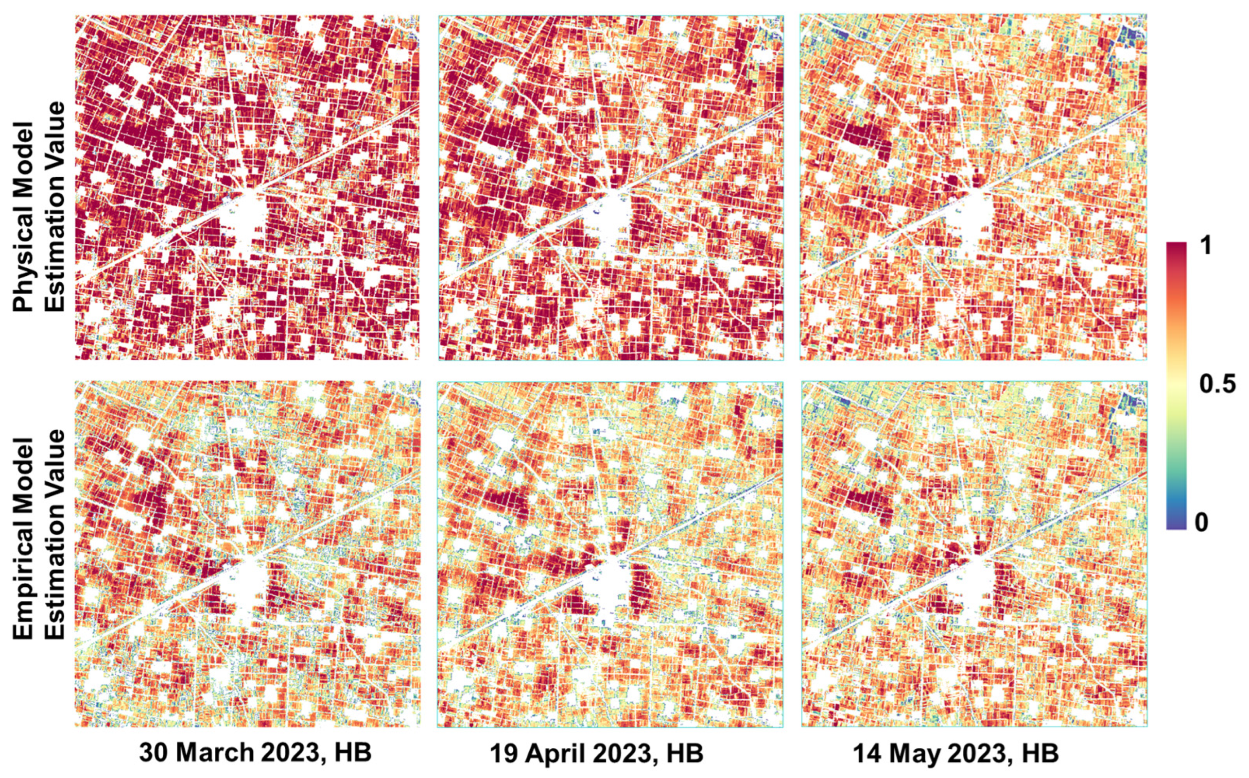
3.3.4. Accuracy Assessment at Satellite Scale

Ground experiments have shown that MNDVI has a stable ability to retrieve $f\mathrm{P}\mathrm{A}\mathrm{R}$, with minimal influence from variations in light conditions, crop varieties, and growth differences, enabling its application in large-scale $f\mathrm{P}\mathrm{A}\mathrm{R}$ retrieval. However, further experiments are needed to verify its accuracy at the satellite scale. Therefore, in this study, three cloud-free 10 m Sentinel-2 images of the SZ during the critical growth stages of winter wheat were selected for accuracy validation. The validation area was chosen as a 1000 ✕ 1000 pixel (10 ✕ 10 km) region, with non-winter wheat areas masked out. All winter wheat pixels in this region were used for validation. The $f\mathrm{P}\mathrm{A}\mathrm{R}$ calculated using the Biophysical Processor tool in SNAP 9.0.0 software was used as the ground truth data to verify the reliability of the data obtained from Equation (3). Figure 6 shows the results of the comparison between the actual $f\mathrm{P}\mathrm{A}\mathrm{R}$ and the estimated $f\mathrm{P}\mathrm{A}\mathrm{R}$ during the critical phenological stages. The coefficients of determination for the three stages were 0.718, 0.550, and 0.578, with the lower coefficient in the later stage possibly due to the higher $f\mathrm{P}\mathrm{A}\mathrm{R}$ values. However, overall, the estimated values were lower than the actual values, indicating a certain underestimation phenomenon in this method, which may be caused by vegetation index saturation in the later stages.

In this study, we compare the ability of satellite-scale physical models and the empirical model obtained in this research to retrieve winter wheat $f\mathrm{P}\mathrm{A}\mathrm{R}$ in the southern and eastern parts of the North China Plain, specifically in ZK and Huaibei HB. The $f\mathrm{P}\mathrm{A}\mathrm{R}$ values of the two models were calculated based on Sentinel-2 images during the critical phenological period of winter wheat, and the results are shown in Figure 7 and Figure 8. In ZK, the determination coefficients of the $f\mathrm{P}\mathrm{A}\mathrm{R}$ values estimated by the two models were 0.9003, 0.7818, and 0.6534, while in Huaibei, they were 0.6929, 0.7183, and 0.8312. It can be seen that even at the satellite scale, the $f\mathrm{P}\mathrm{A}\mathrm{R}$ estimated based on MNDVI and the physical model still have a good correlation in different regions and under different planting conditions, further demonstrating the universality of estimating $f\mathrm{P}\mathrm{A}\mathrm{R}$ based on MNDVI.

4. Discussion

4.1. The Necessity of Considering Variety and Water Stress

The current models from existing research have not accounted for differences in varieties and water stress. Therefore, further validation is needed to determine whether the $f\mathrm{P}\mathrm{A}\mathrm{R}$ estimation model based on the vegetation index will produce accuracy differences under different varieties and water stress. For instance, the estimation model conducted by the variety of T3 should be applied to T11 to test its suitability among different varieties. Similarly, the models based on one IS also should be assessed by other ISs to ensure the necessity of considering water stress or not.

The correlation model between the vegetation index MNDVI and $f\mathrm{P}\mathrm{A}\mathrm{R}$ based on T3 is Equation (5).

$$f\mathrm{P}\mathrm{A}\mathrm{R}=1.4198\times \mathrm{M}\mathrm{N}\mathrm{D}\mathrm{V}\mathrm{I}-0.4126,$$

(5)

It was found that the model achieved R of 0.710 when used to estimate T3, as shown in Figure 9a. However, when this model was used to estimate the fPAR of variety T11, some plots had estimated $f\mathrm{P}\mathrm{A}\mathrm{R}$ values less than 0, as shown in Figure 9b, which is an incorrect estimation result. Similarly, Equation (6) is based on IS1 to establish a correlation model between MNDVI and $f\mathrm{P}\mathrm{A}\mathrm{R}$.

$$f\mathrm{P}\mathrm{A}\mathrm{R}=0.3647\times \mathrm{M}\mathrm{N}\mathrm{D}\mathrm{V}\mathrm{I}+0.535,$$

(6)

When using the measurement value of IS-A for accuracy verification, the RMSE is 0.077, as shown in Figure 9c, while when using IS-G for verification, the RMSE is 0.245, as shown in Figure 9d. It can be seen that without considering the differences in variety and water stress, there will be significant errors in the estimation results and even unreasonable estimation values. This indicates the need to consider the differences in variety and water stress.

4.2. Sensitivity Analysis of MNDVI

In the current study, $f\mathrm{P}\mathrm{A}\mathrm{R}$ in the light use efficiency model is often calculated based on NDVI, for example in EC-LUE [35] where $f\mathrm{P}\mathrm{A}\mathrm{R}=1.24\times \mathrm{N}\mathrm{D}\mathrm{V}\mathrm{I}-0.168$. This study believes that MNDVI may have greater advantages; therefore, we compared the two vegetation indices and analyzed the response differences in winter wheat growth during the winter wheat growing season. Therefore, we compared it with NDVI to analyze the differences between the two vegetation indices during the growth process of winter wheat. The current study indicates that NDVI shows saturation in estimating $f\mathrm{P}\mathrm{A}\mathrm{R}$ during the peak growth period of crops [36], making it difficult to estimate accurately. Therefore, based on the MODIS daily reflectance data product (MCD43A4), we compared the variations of pure winter wheat pixels in the North China Plain from 1 January to 30 June to analyze the saturation status of the two vegetation indices. Figure 10 shows the time series curves of NDVI and MNDVI after being filtered by a moving average window of size 5, as well as the absolute values of their slopes during different periods.

From Figure 10, it can be seen that the range of MNDVI is approximately −0.1 to 0.75 with a range of 0.85, while NDVI ranges from 0.25 to 0.85 with a range of 0.6. The absolute values of the slopes of MNDVI are also greater than those of NDVI throughout the growth cycle. Even after winter wheat has reached the jointing stage, when NDVI changes less and the absolute value of the slope is smaller, MNDVI still has a larger slope and continues to show a changing trend. The above two points indicate that, compared to NDVI, firstly, MNDVI is more sensitive to vegetation growth changes, and the differences in vegetation growth changes are more pronounced for MNDVI. Secondly, MNDVI is less prone to saturation and even after the jointing stage of winter wheat, there are still significant changes in MNDVI. Therefore, MNDVI has an advantage in estimating $f\mathrm{P}\mathrm{A}\mathrm{R}$.

4.3. The Potential of MNDVI in Estimating Winter Wheat Yield

The $f\mathrm{P}\mathrm{A}\mathrm{R}$ estimation results at the satellite scale reveal the MNDVI-based model for estimating large $f\mathrm{P}\mathrm{A}\mathrm{R}$ proposed in this study has a certain underestimation at the beginning or end of major phenological periods when compared with physical models. This underestimation phenomenon may still be caused by MNDVI saturation, although MNDVI is relatively less susceptible to saturation as compared with NDVI. Therefore, in future research, it is the key to find a vegetation index that can be less prone to saturation for improving the estimation accuracy of $f\mathrm{P}\mathrm{A}\mathrm{R}$.

From

Table A1. Empirical models of vegetation index with $f\mathrm{P}\mathrm{A}\mathrm{R}$ in existing studies.

VI	Equation	Vegetation Type
NDVI	$f\mathrm{P}\mathrm{A}\mathrm{R}=1.24\times \mathrm{N}\mathrm{D}\mathrm{V}\mathrm{I}-0.168$	Winter wheat [35]
Red edge NDVI	$fPAR=1.25\times \mathrm{R}\mathrm{e}\mathrm{N}\mathrm{D}\mathrm{V}\mathrm{I}-0.10$; $f\mathrm{P}\mathrm{A}\mathrm{R}={f\mathrm{P}\mathrm{A}\mathrm{R}}_{\mathrm{m}\mathrm{a}\mathrm{x}}\times f\left(\mathrm{N}\mathrm{D}\mathrm{V}\mathrm{I}\right)$; ${f\mathrm{P}\mathrm{A}\mathrm{R}}_{\mathrm{m}\mathrm{a}\mathrm{x}}=0.95$	Cron, soybean [40]
NDVI	$f\left(NDVI\right)=\max \left(\min \left(\frac{\mathrm{n}\mathrm{d}\mathrm{v}\mathrm{i} - 0.1}{0.9 - 0.1},1\right),0\right)$	Grassland, farmland and forest [41]
NDVI	$f\mathrm{P}\mathrm{A}\mathrm{R}=1.0\times \mathrm{N}\mathrm{D}\mathrm{V}\mathrm{I}-0.05$	Forest [42]
GNDVI	$f\mathrm{P}\mathrm{A}\mathrm{R}=0.1825{\mathrm{e}}^{1.8588\times \mathrm{G}\mathrm{N}\mathrm{D}\mathrm{V}\mathrm{I}}$	Cron [43]
MTCI	$f\mathrm{P}\mathrm{A}\mathrm{R}=0.72\times \mathrm{M}\mathrm{T}\mathrm{C}\mathrm{I}+0.08$	Cron and forest [44]
VARI	$f\mathrm{P}\mathrm{A}\mathrm{R}=1.314\times \mathrm{V}\mathrm{A}\mathrm{R}\mathrm{I}+0.189$	Grassland [45]
NDPI	$f\mathrm{P}\mathrm{A}\mathrm{R}=0.972\times \mathrm{N}\mathrm{D}\mathrm{P}\mathrm{I}-0.028$	Grassland [32]

, it can be seen that different vegetation $f\mathrm{P}\mathrm{A}\mathrm{R}$ have different linear relationships with vegetation indices. Even for the same vegetation type, there are variations in the linear relationship between different vegetation indices and $f\mathrm{P}\mathrm{A}\mathrm{R}$. Different research areas, even with the same crop and different vegetation indices, have obtained different linear relationships. This may be due to differences in observation conditions, satellite data, and even different phenological stages, which can lead to differences in linear relationships [27]. In the North China region, which is mainly characterized by smallholder agriculture, there is a complex cropping structure, different winter wheat varieties, significant climatic variations, and a wide range of phenological stages. If a model is established to relate vegetation indices to $f\mathrm{P}\mathrm{A}\mathrm{R}$ based on a specific region or variety of winter wheat, it may result in significant differences in $f\mathrm{P}\mathrm{A}\mathrm{R}$ estimation for the entire region. Therefore, in order to improve the accuracy of winter wheat $f\mathrm{P}\mathrm{A}\mathrm{R}$ calculation in the North China Plain and to improve the accuracy of winter wheat yield estimation, it is necessary to find vegetation indices that are stable throughout the phenological period and more suitable for $f\mathrm{P}\mathrm{A}\mathrm{R}$ estimation in the North China Plain. This will enable the construction of a more universally applicable fitting model to improve the accuracy of wheat yield estimation.

The present study uses simulated Sentinel-2 reflectance data to find that the MNDVI-based index model has high stability and good applicability in estimating winter wheat $f\mathrm{P}\mathrm{A}\mathrm{R}$. Moreover, the computation of MNDVI requires only the use of near-infrared and red-band reflectance data, which allows the acquisition of $f\mathrm{P}\mathrm{A}\mathrm{R}$ data with a spatial resolution of 10 m. This has significant application value in agricultural monitoring of regions with complex crop structures, such as the North China Plain. In particular, it can be combined with existing vegetation index downscaling algorithms, such as STARFM [37] and CRC [38], to reconstruct high spatiotemporal resolution vegetation index data and thereby calculate high spatiotemporal resolution $f\mathrm{P}\mathrm{A}\mathrm{R}$ data. This is of great reference value for agricultural monitoring in cloudy and rainy areas.

Due to the difficulty in obtaining high spatiotemporal resolution $f\mathrm{P}\mathrm{A}\mathrm{R}$ data, existing light use efficiency models mostly rely on 8-day, 15-day, or monthly averages to estimate crop yield. For example, EC-LUE uses Landsat 7/8 to estimate $f\mathrm{P}\mathrm{A}\mathrm{R}$ based on NDVI every 8 days [39], which can introduce significant errors in the calculation results. If high spatio-temporal resolution $f\mathrm{P}\mathrm{A}\mathrm{R}$ data can be obtained and combined with light use efficiency models for winter wheat yield estimation, it can improve the accuracy of yield estimation.

5. Conclusions

In this study, we first simulated Sentinel-2 satellite reflectance based on ground ASD data and compared the correlation between commonly used vegetation indices and photosynthetically active radiation at different observation dates. Secondly, we constructed an index correlation model based on MNDVI throughout the critical growth period and validated the accuracy of the $f\mathrm{P}\mathrm{A}\mathrm{R}$ estimation using the model under different crop varieties, observation dates, and water stress conditions. Finally, we compared it with the commonly used vegetation index NDVI and carried out a sensitivity analysis. The main conclusions of this study are as follows: (1) due to differences in observation conditions and crop characteristics, the correlation between vegetation indices and $f\mathrm{P}\mathrm{A}\mathrm{R}$ can vary; (2) the index model based on MNDVI is the most stable and accurate model, with a coefficient of determination for $f\mathrm{P}\mathrm{A}\mathrm{R}$ throughout the critical growth period of winter wheat reaching 0.6649. Under different cultivars, observation dates, and water stress conditions, the highest coefficients of determination can reach 0.918, 0.881, and 0.830, with the lowest RMSE being 0.088, 0.096, and 0.089. At the satellite scale, the highest coefficient of determination is 0.8321; (3) MNDVI is more sensitive to changes in winter wheat growth and less prone to saturation compared to NDVI. In conclusion, using MNDVI for $f\mathrm{P}\mathrm{A}\mathrm{R}$ estimation during the critical growth period of winter wheat can provide good estimation results, and the estimation accuracy is less affected by internal and external factors.

This study’s results demonstrate the feasibility of using high spatial resolution $f\mathrm{P}\mathrm{A}\mathrm{R}$ estimation for winter wheat based on Sentinel-2 vegetation indices. By using MNDVI, it is possible to quickly and accurately obtain $f\mathrm{P}\mathrm{A}\mathrm{R}$ data with a spatial resolution of 10 m. This can assist in near real-time agricultural monitoring and provide a reference for rapid crop yield estimation.

References

1. Tripathi, A.; Tripathi, D.K.; Chauhan, D.K.; Kumar, N.; Singh, G.S. Paradigms of climate change impacts on some major food sources of the world: A review on current knowledge and future prospects. Agric. Ecosyst. Environ. 2016, 216, 356–373. [Google Scholar] [CrossRef]
2. Khan, S.; Hanjra, M.A.; Mu, J. Water management and crop production for food security in China: A review. Agric. Water Manag. 2009, 96, 349–360. [Google Scholar] [CrossRef]
3. Gao, F.; Zhang, X. Mapping crop phenology in near real-time using satellite remote sensing: Challenges and opportunities. J. Remote Sens. 2021, 14, 8379391. [Google Scholar] [CrossRef]
4. Bolton, D.K.; Friedl, M.A. Forecasting crop yield using remotely sensed vegetation indices and crop phenology metrics. Agric. For. Meteorol. 2013, 173, 74–84. [Google Scholar] [CrossRef]
5. Liu, C.A.; Chen, Z.X.; Yun, S.H.A.O.; Chen, J.S.; Hasi, T.; Pan, H.Z. Research advances of SAR remote sensing for agriculture applications: A review. J. Integr. Agric. 2019, 18, 506–525. [Google Scholar] [CrossRef]
6. Sun, L.; Gao, F.; Anderson, M.C.; Kustas, W.P.; Alsina, M.M.; Sanchez, L.; Sams, B.; McKee, L.; Dulaney, W.; White, W.; et al. Daily Mapping of 30 m LAI and NDVI for Grape Yield Prediction in California Vineyards. Remote Sens. 2017, 9, 317. [Google Scholar] [CrossRef]
7. Xiao, X.; Zhang, Q.; Braswell, B.; Urbanski, S.; Boles, S.; Wofsy, S.; Moore, B., III; Ojima, D. Modeling gross primary production of temperate deciduous broadleaf forest using satellite images and climate data. Remote Sens. Environ. 2004, 91, 256–270. [Google Scholar] [CrossRef]
8. Huang, J.; Ma, H.; Sedano, F.; Lewis, P.; Liang, S.; Wu, Q.; Zhu, D. Evaluation of regional estimates of winter wheat yield by assimilating three remotely sensed reflectance datasets into the coupled WOFOST–PROSAIL model. Eur. J. Agron. 2019, 102, 1–13. [Google Scholar] [CrossRef]
9. Xiao, G.; Zhang, X.; Niu, Q.; Li, X.; Li, X.; Zhong, L.; Huang, J. Winter wheat yield estimation at the field scale using Sentinel-2 data and deep learning. Comput. Electron. Agric. 2024, 216, 108555. [Google Scholar] [CrossRef]
10. Wang, X.; Huang, J.; Feng, Q.; Yin, D. Winter Wheat Yield Prediction at County Level and Uncertainty Analysis in Main Wheat-producing Regions of China with Deep Learning Approaches. Remote Sens. 2020, 12, 1744. [Google Scholar] [CrossRef]
11. Yuan, W.; Liu, S.; Yu, G.; Bonnefond, J.-M.; Chen, J.; Davis, K.; Desai, A.R.; Goldstein, A.H.; Gianelle, D.; Rossi, F.; et al. Global estimates of evapotranspiration and gross primary production based on MODIS and global meteorology data. Remote Sens. Environ. 2010, 114, 1416–1431. [Google Scholar] [CrossRef]
12. D’Odorico, P.; Gonsamo, A.; Pinty, B.; Gobron, N.; Coops, N.; Mendez, E.; Schaepman, M.E. Intercomparison of fraction of absorbed photosynthetically active radiation products derived from satellite data over Europe. Remote Sens. Environ. 2014, 142, 141–154. [Google Scholar] [CrossRef]
13. Pei, Y.; Dong, J.; Zhang, Y.; Yuan, W.; Doughty, R.; Yang, J.; Zhou, D.; Zhang, L.; Xiao, X. Evolution of light use efficiency models: Improvement, uncertainties, and implications. Agric. For. Meteorol. 2022, 317, 108905. [Google Scholar] [CrossRef]
14. Prince, S.D.; Goward, S.N. Global primary production: A remote sensing approach. J. Biogeogr. 1995, 22, 815–835. [Google Scholar] [CrossRef]
15. Peng, D.; Zhang, B.; Liu, L. Comparing spatiotemporal patterns in Eurasian FPAR derived from two NDVI-based methods. Int. J. Digit. Earth 2012, 5, 283–298. [Google Scholar] [CrossRef]
16. Chen, J.M. Canopy architecture and remote sensing of the fraction of photosynthetically active radiation absorbed by boreal conifer forests. IEEE Trans. Geosci. Remote Sens. 1996, 34, 1353–1368. [Google Scholar] [CrossRef]
17. Zhou, G.; Liu, X.; Zhao, S.; Liu, M.; Wu, L. Estimating FAPAR of rice growth period using radiation transfer model coupled with the WOFOST model for analyzing heavy metal stress. Remote Sens. 2017, 9, 424. [Google Scholar] [CrossRef]
18. Xiao, Z.; Liang, S.; Sun, R.; Wang, J.; Jiang, B. Estimating the fraction of absorbed photosynthetically active radiation from the MODIS data based GLASS leaf area index product. Remote Sens. Environ. 2015, 171, 105–117. [Google Scholar] [CrossRef]
19. Zhou, Q.; Fellows, A.; Flerchinger, G.N.; Flores, A.N. Examining interactions between and among predictors of net ecosystem exchange: A machine learning approach in a semi-arid landscape. Sci. Rep. 2019, 9, 2222. [Google Scholar] [CrossRef] [PubMed]
20. Myneni, R.; Knyazikhin, Y. MODIS/Terra+Aqua Leaf Area Index/FPAR 4-Day L4 Global 500 m SIN Grid. Available online: https://lpdaac.usgs.gov/products/mcd15a3hv061/ (accessed on 15 January 2020).
21. Xiao, Z.; Liang, S.; Wang, J.; Chen, P.; Yin, X.; Zhang, L.; Song, J. Use of general regression neural networks for generating the GLASS leaf area index product from time-series MODIS surface reflectance. IEEE Trans. Geosci. Remote Sens. 2013, 52, 209–223. [Google Scholar] [CrossRef]
22. Jin, H.; Li, A.; Liang, S.; Ma, H.; Xie, X.; Liu, T.; He, T. Generating high spatial resolution GLASS FAPAR product from Landsat images. Sci. Remote Sens. 2022, 6, 100060. [Google Scholar] [CrossRef]
23. Knyazikhin, Y.; Martonchik, J.V.; Myneni, R.B.; Diner, D.J.; Running, S.W. Synergistic algorithm for estimating vegetation canopy leaf area index and fraction of absorbed photosynthetically active radiation from MODIS and MISR data. J. Geophys. Res. Atmos. 1998, 103, 32257–32275. [Google Scholar] [CrossRef]
24. Gobron, N.; Pinty, B.; Aussedat, O.; Taberner, M.; Faber, O.; Mélin, F.; Lavergne, T.; Robustelli, M.; Snoeij, P. Uncertainty estimates for the FAPAR operational products derived from MERIS—Impact of top-of-atmosphere radiance uncertainties and validation with field data. Remote Sens. Environ. 2008, 112, 1871–1883. [Google Scholar] [CrossRef]
25. Wang, Y.; Tian, Y.; Zhang, Y.; El-Saleous, N.; Knyazikhin, Y.; Vermote, E.; Myneni, R.B. Investigation of product accuracy as a function of input and model uncertainties: Case study with SeaWiFS and MODIS LAI/FPAR algorithm. Remote Sens. Environ. 2001, 78, 299–313. [Google Scholar] [CrossRef]
26. Baret, F.; Weiss, M.; Lacaze, R.; Camacho, F.; Makhmara, H.; Pacholcyzk, P.; Smets, B. GEOV1: LAI and FAPAR essential climate variables and FCOVER global time series capitalizing over existing products. Part1: Principles of development and production. Remote Sens. Environ. 2013, 137, 299–309. [Google Scholar] [CrossRef]
27. Tian, D.; Fan, W.; Ren, H. Progress of fraction of absorbed photosynthetically active radiation retrieval from remote sensing data. J. Remote Sens. 2020, 24, 1307–1324. [Google Scholar] [CrossRef]
28. Cheng, Y.B.; Zhang, Q.; Lyapustin, A.I.; Wang, Y.; Middleton, E.M. Impacts of light use efficiency and fPAR parameterization on gross primary production modeling. Agric. For. Meteorol. 2014, 189, 187–197. [Google Scholar] [CrossRef]
29. Zeng, Y.; Hao, D.; Park, T.; Zhu, P.; Huete, A.; Myneni, R.; Knyazikhin, Y.; Qi, J.; Nemani, R.R.; Li, F.; et al. Structural complexity biases global vegetation greenness measures. Nat. Ecol. Evol. 2023, 7, 1790–1798. [Google Scholar] [CrossRef]
30. Chen, Z.; Shao, Q.; Liu, J.; Wang, J. Analysis of net primary productivity of terrestrial vegetation on the Qinghai-Tibet Plateau, based on MODIS remote sensing data. Sci. China Earth Sci. 2012, 55, 1306–1312. [Google Scholar] [CrossRef]
31. Pei, Y.; Dong, J.; Zhang, Y.; Yang, J.; Zhang, Y.; Jiang, C.; Xiao, X. Performance of four state-of-the-art GPP products (VPM, MOD17, BESS and PML) for grasslands in drought years. Ecol. Inform. 2020, 56, 101052. [Google Scholar] [CrossRef]
32. Ding, L.; Li, Z.; Shen, B.; Wang, X.; Xu, D.; Yan, R.; Yan, Y.; Xin, X.; Xiao, J.; Li, M.; et al. Spatial patterns and driving factors of aboveground and belowground biomass over the eastern Eurasian steppe. Sci. Total Environ. 2022, 803, 149700. [Google Scholar] [CrossRef]
33. Dong, T.; Meng, J.; Shang, J.; Liu, J.; Wu, B. Evaluation of chlorophyll-related vegetation indices using simulated Sentinel-2 data for estimation of crop fraction of absorbed photosynthetically active radiation. IEEE J. Sel. Top. Appl. Earth Obs. Remote Sens. 2015, 8, 4049–4059. [Google Scholar] [CrossRef]
34. Ren, J.; Zhang, N.; Liu, X.; Wu, S. Estimation of Harvest Index of Winter Wheat Based on Simulated Sentinel-2A Reflectance Data and Its Real Remote Sensing Imagery. Trans. Chin. Soc. Agric. Mach. 2022, 53, 231–243. [Google Scholar]
35. Dong, J.; Lu, H.; Wang, Y.; Ye, T.; Yuan, W. Estimating winter wheat yield based on a light use efficiency model and wheat variety data. ISPRS J. Photogramm. Remote Sens. 2020, 160, 18–32. [Google Scholar] [CrossRef]
36. Jenkins, J.P.; Richardson, A.D.; Braswell, B.H.; Ollinger, S.V.; Hollinger, D.Y.; Smith, M.L. Refining light-use efficiency calculations for a deciduous forest canopy using simultaneous tower-based carbon flux and radiometric measurements. Agric. For. Meteorol. 2007, 143, 64–79. [Google Scholar] [CrossRef]
37. Gao, F.; Masek, J.; Schwaller, M.; Hall, F. On the blending of the Landsat and MODIS surface reflectance: Predicting daily Landsat surface reflectance. IEEE Trans. Geosci. Remote Sens. 2006, 44, 2207–2218. [Google Scholar]
38. Sun, L.; Gao, F.; Xie, D.; Anderson, M.; Chen, R.; Yang, Y.; Yang, Y.; Chen, Z. Reconstructing daily 30 m NDVI over complex agricultural landscapes using a crop reference curve approach. Remote Sens. Environ. 2021, 253, 112156. [Google Scholar] [CrossRef]
39. Yuan, W.; Liu, S.; Zhou, G.; Zhou, G.; Tieszen, L.L.; Baldocchi, D.; Bernhofer, C.; Gholz, H.; Goldstein, A.H.; Goulden, M.L.; et al. Deriving a light use efficiency model from eddy covariance flux data for predicting daily gross primary production across biomes. Agric. For. Meteorol. 2007, 143, 189–207. [Google Scholar] [CrossRef]
40. Gitelson, A.A. Remote estimation of fraction of radiation absorbed by photosynthetically active vegetation: Generic algorithm for maize and soybean. Remote Sens. Lett. 2019, 10, 283–291. [Google Scholar] [CrossRef]
41. Yebra, M.; Van Dijk, A.I.; Leuning, R.; Guerschman, J.P. Global vegetation gross primary production estimation using satellite-derived light-use efficiency and canopy conductance. Remote Sens. Environ. 2015, 163, 206–216. [Google Scholar] [CrossRef]
42. Wang, S.; Ibrom, A.; Bauer-Gottwein, P.; Garcia, M. Incorporating diffuse radiation into a light use efficiency and evapotranspiration model: An 11-year study in a high latitude deciduous forest. Agric. For. Meteorol. 2018, 248, 479–493. [Google Scholar] [CrossRef]
43. Tan, C.; Samanta, A.; Jin, X.; Tong, L.; Ma, C.; Guo, W.; Knyazikhin, Y.; Myneni, R.B. Using hyperspectral vegetation indices to estimate the fraction of photosynthetically active radiation absorbed by corn canopies. Int. J. Remote Sens. 2013, 34, 8789–8802. [Google Scholar] [CrossRef]
44. Ogutu, B.O.; Dash, J. An algorithm to derive the fraction of photosynthetically active radiation absorbed by photosynthetic elements of the canopy (FAPAR ps) from eddy covariance flux tower data. New Phytol. 2013, 197, 511–523. [Google Scholar] [CrossRef]
45. Cristiano, P.M.; Posse, G.; Di Bella, C.M.; Jaimes, F.R. Uncertainties in fPAR estimation of grass canopies under different stress situations and differences in architecture. Int. J. Remote Sens. 2010, 31, 4095–4109. [Google Scholar] [CrossRef]
Figure 1. RGB image of the research area captured by UAV on 5 August 2023 and the distribution of varieties in all plots of each IS.
Remotesensing 16 00362 g001
Figure 2. Scheme of ground measurement method of f P A R .
Remotesensing 16 00362 g002
Figure 3. Validation of estimation accuracy of index model based on MNDVI in different varieties.
Remotesensing 16 00362 g003
Figure 4. Validation of estimation accuracy of index model based on MNDVI in different light conditions and phenological stages.
Remotesensing 16 00362 g004
Figure 5. Validation of estimation accuracy of index model based on MNDVI in different irrigation schemes.
Remotesensing 16 00362 g005
Figure 6. Comparison of MNDVI estimation results and true values on satellite scale in SZ.
Remotesensing 16 00362 g006
Figure 7. Comparison of MNDVI estimation results and true values on satellite scale in ZK.
Remotesensing 16 00362 g007
Figure 8. Comparison of MNDVI estimation results and true values on satellite scale in HB.
Remotesensing 16 00362 g008
Figure 9. The impact of considering differences in water stress and variety on the accuracy of f P A R estimation. (a) Establish relevant models based on measurement data from T3; (b) Validate the estimation accuracy of the models using measurement data from T11; (c) Establish relevant models based on measurement data from IS-A; (d) Validate the estimation accuracy of the models using measurement data from IS-G.
Remotesensing 16 00362 g009
Figure 10. Comparison of MNDVI and NDVI response to changes in winter wheat growth.
Remotesensing 16 00362 g010