
An Open Benchmark Dataset for Forest Characterization from Sentinel-1 and -2 Time Series

1
Geoinformatics Department, Hochschule München University of Applied Sciences, Karlstraße 6, D-80333 Munich, Germany
2
Institute for Applications of Machine Learning and Intelligent Systems (IAMLIS), Lothstraße 34, D-80335 Munich, Germany
*
Author to whom correspondence should be addressed.
†
These authors contributed equally to this work.
Remote Sens. 2024, 16(3), 488; https://doi.org/10.3390/rs16030488
Submission received: 9 November 2023
/
Revised: 15 January 2024
/
Accepted: 19 January 2024
/
Published: 26 January 2024
(This article belongs to the Special Issue Remote Sensing for Forest Morphological and Physiological Traits Monitoring)
Abstract
:Earth observation satellites offer vast opportunities for quantifying landscapes and regional land cover composition and changes. The integration of artificial intelligence in remote sensing is essential for monitoring significant land cover types like forests, demanding a substantial volume of labeled data for effective AI model development and validation. The Wald5Dplus project introduces a distinctive open benchmark dataset for mid-European forests, labeling Sentinel-1/2 time series using data from airborne laser scanning and multi-spectral imagery. The freely accessible satellite images are fused in polarimetric, spectral, and temporal domains, resulting in analysis-ready data cubes with 512 channels per year on a 10 m UTM grid. The dataset encompasses labels, including tree count, crown area, tree types (deciduous, coniferous, dead), mean crown volume, base height, tree height, and forested area proportion per pixel. The labels are based on an individual tree characterization from high-resolution airborne LiDAR data using a specialized segmentation algorithm. Covering three test sites (Bavarian Forest National Park, Steigerwald, and Kranzberg Forest) and encompassing around six million trees, it generates over two million labeled samples. Comprehensive validation, including metrics like mean absolute error, median deviation, and standard deviation, in the random forest regression confirms the high quality of this dataset, which is made freely available.
1. Introduction
Amidst the growing recognition of the immense value of forest ecosystems in combating climate change and supporting biodiversity, the demand for rapid, precise, and robust methods to monitor these vital ecosystems is on the rise [1]. Forests, which shelter the majority of terrestrial biodiversity, span approximately 4.06 billion hectares, covering 31% of the world’s land surface. They function as crucial carbon reservoirs and play an indispensable role in climate regulation [2]. To effectively track the progress toward these goals, as well as to monitor deforestation, degradation, and forest responses to climate change, there is an increasing need for large-scale, cost-effective monitoring, ideally with automated data collection and processing up to the final information product. In the last decade, there has been a notable increase in the accessibility and application of remote sensing (RS) technologies, providing data with resolutions sufficiently fine to discern individual trees, as demonstrated in various references employing high-resolution data [3,4,5,6,7,8,9,10,11]. While this presents opportunities for enhancing our understanding of forests, it also poses challenges in data interpretation [12,13].
The field’s expansion has resulted in an influx of intricate datasets, demanding the development of innovative data science approaches to efficiently extract ecologically significant information. Additionally, the lack of universally acknowledged benchmarking datasets has impeded methodological advancement and posed difficulties in comparing different studies [14]. This perspective underscores the advantages of establishing and applying benchmarking datasets while outlining the key attributes that can optimize their value for the wider scientific community.
The collaboration between remote sensing (RS) and forestry practices is gaining prominence in the field of forest management, highlighting the interdependence of these domains [15,16,17]. This dynamic interaction harnesses the capabilities of machine learning (ML) and deep learning (DL) to effectively handle the extensive and diverse datasets inherent in RS images. ML and DL techniques play a crucial role in simplifying complex image information, such as discerning a single pixel as a coniferous tree through intricate time-series analysis. Despite their prowess, these techniques require careful hyperparameterization to address data variability and imperfections. While offering optimal adaptation to specific challenges, this adaptability introduces considerations such as the risk of overfitting [18], thereby necessitating a substantial number of training samples, akin to the layers of a deep neural network.
Three primary approaches are prevalent for acquiring a substantial number of training samples: (1) crafting comprehensive training datasets, often indispensable for DL approaches that require extensive training data. In contrast, some ML methods can work effectively with smaller datasets. (2) Employing data augmentation to introduce artificial data variations [19]. (3) Utilizing pre-trained networks with supplementary adaptation layers.
Ongoing research explores capitalizing on symmetries and commonalities within network layers to enhance decision making and model robustness. However, methods (2) and (3) entail manual, non-standardized alterations to either the training data or the network architecture, making them suitable for specific applications but unsuitable for benchmarking ML and DL algorithms.
Therefore, extensive training datasets (1) are indispensable, enabling the training of new algorithms, potentially even without prior knowledge, similar to pre-trained networks. Several benchmark datasets are available to facilitate advancements in the field. Further research endeavors to leverage symmetries and similarities within network layers to enhance or simplify decision making through the analysis of model zoos [20]. While predominantly applied in DL, these techniques are less common in conventional ML, highlighting a key difference between the two: the flexibility and depth of DL networks, enabling the exploitation of symmetries and commonalities.
As both (2) and (3) require manual and non-standardized modifications of the training data (2) and/or the network (3), they are well suited for specific applications but not for ranking ML and DL algorithms. This underscores the need for standardized and extensive training datasets, particularly when benchmarking the performance of various ML and DL models in forest management.
1.1. Related Benchmark Datasets
Back in 2018, the International Society for Photogrammetry and Remote Sensing (ISPRS) published true orthophotos and surface models together with semantic labels describing the apparent land cover class like impervious surface, building, low vegetation, tree, car [21]. These datasets have already been widely used for the testing and ranking of machine learning algorithms.
Recently, a new multimodal benchmark dataset for RS (MDAS) was added to the ML4Earth platform that comprises SAR, multi-spectral, and hyper-spectral imagery, as well as a surface model [22]. The annotation provides pavement, low vegetation, soil, tree, roof, and water as labels. This dataset is dedicated to the use of satellite data by Sentinel-1 and -2 and EnMAP [23].
The focus of all benchmark datasets so far—to the best of our knowledge—lies on the semantic interpretation, i.e., distinct classes in a nominal scale are assigned.
Contrastingly, high-resolution remote sensing imagery (HR-RSI) benchmark datasets released in recent years, including WHU-RS19 [24], UC Merced [25,26], PatternNet [13], and RESISC-45 [27], focus on object classes and have proven successful for classification tasks. The diversity in structure and design of these datasets presents a unique opportunity to explore the utility of combining them into a larger meta-dataset (MDS) [28], addressing challenges such as heterogeneous image sizes within class and varied spatial resolution within class.
Adding to this landscape, several new benchmark datasets complement these efforts: ReforesTree [1] focuses on forest carbon stock estimation within carbon offsetting certification standards, outperforming satellite-based estimates. Addressing tree species classification in central Europe, TreeSatAI [29] leverages multi-sensor data. Designed for training deep neural networks, Barknet 1.0 [30] comprises over 23,000 high-resolution bark images from 23 different tree species in eastern seaboard forests of Canada. NeonTreeEvaluation Benchmark Data [31] assess crown detection in the United States using RGB, LiDAR, and hyper-spectral data. LuoJiaSET [32] is a large-scale training sample database system for intelligent interpretation of remote sensing imagery.
Moreover, the OpenEarthMap dataset [33] introduces a benchmark for global high-resolution land cover mapping, comprising 2.2 million segments of 5000 aerial and satellite images. With manually annotated eight-class land cover labels at a 0.25–0.5 m ground sampling distance, OpenEarthMap allows semantic segmentation models trained on it to generalize worldwide, providing a valuable resource for advancing remote sensing methodologies.
The next step from a mathematical point of view is the use of parameters in cardinal scale. This leads directly to a regression approach because not distinct classes but continuous values have to be predicted from satellite data. Such a dataset—and especially for forest characterization—has not been presented so far. This is exactly the point where our project idea of Wald5Dplus comes into play: the creation of a labeled benchmark for forest characterization, not classification. Continuous parameters like the crown area per tree type, the tree height, and the crown volume amongst others are attached to each pixel in the ARD cube. The annotation of parameters in cardinal scale places new demands on the labeling that are briefly explained in the following.
1.2. Requirements on Training Data
In the domain of RS and the application of AI techniques, a series of imperative requirements concerning training data come to the fore. These requisites hold considerable significance, especially within the context of RS, encompassing both general and forest-specific aspects.
High-Quality and Well-Labeled Data: Foremost, a fundamental requirement in the field of RS pertains to the availability of high-quality datasets that are meticulously labeled. This precision ensures that AI algorithms can be effectively trained and validated on information that is both accurate and dependable. It is notable that machine learning, a cornerstone of AI, relies heavily on data quality. This aligns with findings from research emphasizing that the successful utilization of machine learning techniques in RS applications necessitates high-quality data, particularly well-labeled datasets [34]. Such well-labeled data serve as the bedrock upon which AI models can be constructed and validated.
Accessibility of Publicly Available Datasets: A pivotal requirement arises from the accessibility of publicly available datasets, accompanied by validation data. These datasets serve as indispensable benchmarks for the development and validation of algorithms, allowing researchers to evaluate their methods against established standards. This aligns with the notion that publicly available datasets with validation data are crucial for researchers to verify their developed algorithms and compare them with state-of-the-art methods. In various standard RS applications, frequently employed datasets serve as reference points for algorithm testing. The abundance of such datasets underscores the importance of making high-quality training samples available, as highlighted in the literature [14,35,36].
Diversity and Representativeness: Training data should encompass a wide range of scenarios to enable AI models to generalize effectively. This diversity is crucial in the field of RS, where real-world conditions can vary significantly. Machine learning techniques, which are foundational in AI, rely on diverse training data to ensure that models can adapt to different conditions and achieve robust generalization. In this context, the need for variations in land cover, seasonal changes, and different environmental conditions is essential to ensure that AI models can effectively handle the intricacies of RS applications [37].
Spatial and Temporal Coverage: The training dataset should provide comprehensive spatial and temporal coverage [37,38], ensuring that AI models can effectively adapt to diverse regions and monitor temporal dynamics with precision. High-quality training samples, representative of a wide range of geographic locations and temporal changes, are fundamental in addressing the challenges of RS data, especially in the context of forests. The utilization of data with broad spatial and temporal coverage aligns with the need to capture fine-grained spatial and temporal changes in RS applications.
Data Resolution: Training data should align with the spatial and temporal resolution of the RS data used for analysis. This matching resolution is essential for enabling AI models to capture and respond to temporal changes with accuracy, as highlighted in the literature. Aligning training data resolution with RS data resolution is a crucial aspect of ensuring the effective application of AI in RS [14].
Quantity and Sample Size: Adequate training samples are pivotal for optimizing AI models [34,39]. The quantity of training data should align with the complexity of the analysis task and the specific requirements of the AI model under consideration. The importance of having an ample sample size to mitigate the risk of model underfitting is well established in the field of machine learning, including in the realm of RS.
Consistency and Continuity: Consistency in labeling and data quality [38] throughout the training dataset is imperative for ensuring the reliability of AI models in RS tasks, especially those involving time-series data. Additionally, maintaining continuity in data collection is essential for effectively monitoring changes and trends. Such consistency and continuity are essential components of robust AI model development, as recognized in the existing body of literature.
Annotated Metadata: Annotated metadata [14,32], providing comprehensive information regarding the data’s source, acquisition date, geographical location, and any preprocessing steps applied, enhance the interpretability and utility of training data. These metadata are vital in providing context to the training data, enabling researchers to better understand the information used for AI model development. Researchers in the field have acknowledged the critical role that annotated metadata play in the effective utilization of training data.
Data Balance: Maintaining a balanced representation of classes or categories within training data is vital, especially in classification tasks. Unbalanced datasets can present a substantial obstacle in the process of model optimization, especially when specific classes are infrequent or not well represented [38,40]. Ensuring equitable representation of classes is a recognized strategy to prevent biases and skewed results. Achieving data balance is crucial for accurate classification of RS data, a concept well supported by prior research [34].
In summary, these requirements collectively underscore the pivotal role of training data in the accuracy and effectiveness of AI models in RS applications, particularly in the forest context. These requirements align with the findings from [34,35,36,37,39] and are fundamental in ensuring that AI techniques are effectively applied to RS data, ultimately advancing the field and promoting robust, reliable, and insightful analyses of RS data.
1.3. Concept of the Wald5Dplus Benchmark Data Cube
In addressing the challenges posed by RS data and the development of a benchmark dataset that integrates RS data and reference data, it is imperative to devise effective strategies. These strategies are vital for ensuring that the benchmark dataset meets the rigorous requirements demanded in the field of ML and DL while also capitalizing on the power of AI techniques. To achieve this, a multifaceted approach has been adopted, which will be described in this section (Figure 1).
The Key Data Source Sentinel: One of the cornerstones of this approach is the utilization of data acquired by the Sentinel satellite missions. Sentinel-1 and Sentinel-2, part of the European Space Agency’s (ESA) Copernicus program, offer substantial advantages. Sentinel-1, through its radar technology, provides insights into the forest canopy, offering a unique view into the dense vegetation. Sentinel-2, on the other hand, offers a view of the forest foliage through multi-spectral imagery. The temporal frequency of data acquisition by these missions, with their weekly and bi-weekly revisit times, provides an ideal basis for monitoring temporal dynamics and capturing variations in forest attributes.
Fusion of Sentinel Data: While both Sentinel-1 and Sentinel-2 (©ESA) sensors offer unique advantages by themselves, the fusion of Sentinel-1 and Sentinel-2 data provides an outstanding opportunity to derive rich information about forest attributes, including tree species and canopy height.
Variability: Variability refers to the diversity and differences present in the input data. In RS, this can manifest as variations in the data captured due to differences in environmental conditions, sensor characteristics, or the objects being observed (e.g., different tree species in a forest). ML algorithms, including AI techniques, thrive when they are exposed to a diverse range of input data. The reason for this is that these algorithms can learn and adapt better when they encounter a wide array of situations and patterns.
For effective training and deployment of AI models, the benchmark dataset aims to address the challenges posed by this variability in RS data. While traditional methodologies often attempted to reduce variability by using techniques like channel combinations (e.g., combining different spectral bands to calculate indices like the NDVI), AI methods are more adept at handling high variability in data. Unlike traditional methods that try to simplify the data by reducing variability, AI techniques have the capability to work with data that exhibit a wide range of attributes, including outliers or extreme data points.
The benchmark dataset leverages the inherent tolerance of AI techniques to diverse data attributes, including those that might deviate significantly from the norm. Rather than eliminating variability, it adapts to it. Additionally, preprocessing techniques are implemented to prepare the data in a format suitable for AI algorithms. This preprocessing may include techniques like explicit normalization, which ensures that data are scaled or adjusted to be in a standardized format [41]. Normalization is particularly important for some machine learning techniques, such as support vector machines, which rely on the data being in a specific range or format to work effectively.
Challenges with Training Data Volume: Generating large training datasets, especially in forest-related applications, presents a unique set of challenges. Unlike land cover identification or agricultural land identification, where readily available datasets such as LUCAS points [42] or INVEKOS data can be employed, forest classification faces distinct challenges. The spatial and temporal heterogeneity in forests, including variations in tree species and canopy height, necessitate extensive and specific training datasets. To address this, the benchmark dataset leverages the copious data provided by Sentinel-1 and Sentinel-2 (©ESA, 2020 and 2021), enhancing the ability to generate large-scale training data. This is particularly important in cases where existing data, such as the Bundeswaldinventur data [43], do not align with the required spatial and temporal coverage for forest classification.
Meeting Training Data Requirements: The benchmark dataset is meticulously crafted to address the multifaceted requirements of training data in the realm of RS and AI applications, capitalizing on the abundance of data from distinct geographical regions, each of vital significance in enhancing the robustness of AI models.
Data Quality and Meticulous Labeling: The cornerstone of this dataset is an unwavering commitment to data quality and meticulous labeling. This ensures that every data point is characterized by a high degree of precision, free from errors, and labeled with painstaking accuracy. The quality of labeling is central to the successful development of AI models. Furthermore, the dataset offers comprehensive and consistent data quality throughout, maintaining the highest standards for accurate and reliable information.
Diversity and Representativeness: To enable AI models to generalize effectively and tackle the intricacies of real-world RS applications, the benchmark dataset encompasses a wide range of forest scenarios. These scenarios span across different geographical regions, including the Bavarian Forest National Park (2016), the Steigerwald Forest (2017), and the Kranzberg Forest (2020), all situated in southeastern Germany (Table 1). While these regions share a common geographical location, they exhibit distinct characteristics due to variations in environmental conditions, tree species, and forest structure. This diversity ensures that AI models can adapt to the heterogeneous nature of RS data and make accurate predictions across a spectrum of scenarios.
Spatial and Temporal Coverage: Comprehensive spatial and temporal coverage is a pivotal aspect of the benchmark dataset. It spans various geographic locations, each with its unique ecological and environmental attributes. Moreover, the dataset captures changes over time, providing temporal dynamics with precision. This broad coverage equips AI models with the ability to adapt to diverse regions and monitor temporal changes, enhancing their capacity to analyze RS data effectively.
Data Resolution: The benchmark dataset is meticulously aligned with the spatial and temporal resolution of RS data used for analysis. This strategic alignment ensures that AI models can effectively process and interpret the level of detail present in RS data. By matching the resolution, the dataset empowers AI models to capture and respond to temporal changes with a high degree of accuracy, contributing to the robustness of their performance.
Quantity and Sample Size: Adequate training samples are pivotal in optimizing AI models for RS applications. The benchmark dataset takes this requirement seriously, ensuring that the quantity of training data is commensurate with the complexity of the analysis task and the specific needs of the AI models under consideration. The provision of large yet manageable training datasets minimizes the risk of model underfitting, fostering the development of accurate and reliable AI models.
This paper emphasizes (1) the development of a unique benchmark dataset, explicitly crafted to meet the exacting requirements in the field of ML and DL, particularly within RS and forest-related applications. By synergistically integrating Sentinel-1 and Sentinel-2 (©ESA, 2020 and 2021) data with AI techniques, it effectively bridges the divide between diverse RS data and AI model application, significantly enhancing the ability to address data variability. The results (2) highlight its success in facilitating the monitoring of forests and a wide array of tree parameters. Moreover, the challenges associated with generating large training datasets are met with a strategic focus on harnessing the capabilities of these satellite missions. By creating large yet manageable training datasets with minimized variability, the benchmark dataset intends to empower AI models to unlock the wealth of information present in RS data, ultimately advancing the field of RS and AI applications in forest contexts.
2. Materials
This section introduces the different databases from which the reference labels and the ARD cube are created.
2.1. Single-Tree Polygons
Within this study, three distinct areas of interest (AOI) were meticulously examined (as illustrated in Figure 2). The reference data employed for analysis correspond to these specific regions, encompassing large parts of the Bavarian Forest National Park [44,45], situated at coordinates 49°15′N, 13°15′E, where the data were acquired via helicopter in 2016, covering a vast expanse of 1443 hectares. Additionally, the study included the Steigerwald Forest [46], located at coordinates 48°25′N, 11°40′E, with data collected using a helicopter in 2017, encapsulating an area of 2600 hectares. Furthermore, the investigation extended to the Kranzberg Forest [47], positioned at coordinates 49°53′N, 10°32′E, where the dataset was acquired through UAVs in 2020, focusing on a more confined seven-hectare terrain. These diverse areas provided a rich and varied dataset essential for the comprehensive analysis conducted within this study.
The reference data, represented in the tree polygons, comprise labeled tree segments, meticulously generated from full-waveform LiDAR and multi-spectral data within the designated research areas in accordance with the specifications delineated in Table 1. The utilization of full-waveform LiDAR data is instrumental in segmenting single trees in different forest layers. The generation of tree segments is achieved through the application of a sophisticated normalized cut algorithm that systematically partitions the LiDAR point cloud into point cloud segments until predefined criteria are met and single trees are found. These tree segments encompass a multitude of calculated attributes, including tree height, crown diameter, crown volume, and crown base height. For a comprehensive elucidation of the reference data creation within the Bavarian forest, Amiri et al. (2019) and Zielewska-Büttner et al. (2018) offer a detailed exposition [44,45].
The tree segmentation generated from the LiDAR point cloud harmoniously integrates with the multi-spectral data to facilitate feature extraction. By employing projected polygons of the segmented trees in combination with multi-spectral data covering the AOIs, a diverse array of classifications and feature sets is deployed, with the overarching goal of distinguishing between deciduous and coniferous trees, in addition to detecting deceased standing trees and snags, as comprehensively discussed in the literature [45].
The individual tree polygons encapsulate critical information pertaining to each tree, encompassing details such as tree type, distinguishing between deciduous and coniferous, or identifying it as deadwood (=standing dead trees and snags). These polygons, which can partially overlap, further provide insights into the tree height and the specific crown base height, as well as the crown volume. Validation of this approach was systematically conducted by Amiri et al. [45] and Krzystek et al. [48].
In a recent study [47], a novel tree detection method based on the detection transformer (DETR) was applied. The results demonstrated the potential of this approach, with F1-scores of 83% for coniferous, 86% for mixed, and 71% for deciduous plots, significantly outperforming four baseline methods in all forest types.
In summation, these validation endeavors affirm the robustness and adaptability of this approach across a spectrum of forest structures and environmental conditions. The holistic integration of full-waveform LiDAR data, adaptive algorithms, and advanced instance segmentation techniques collectively embodies the potential to markedly elevate the precision of tree segmentation. This heralds a notable stride forward in the realm of RS and forest-focused applications.
2.2. Sentinel-1/2 Time Series
The key conditions for the choice of satellite are: public availability without costs, high temporal as well as high spatial resolution, and sufficient coverage for larger forest stands. These requirements are fulfilled by the Sentinel-1/2 (©ESA) missions of the Copernicus program. Due to the open data policy of ESA, anyone can download and evaluate the data, which is a crucial step for the extensive use of the knowledge gained by training on the reference data. The short repeat pass times enabled by two satellite sensors on the same orbit in space guarantee weekly acquisitions in the case of the weather-independent SAR sensors Sentinel-1a and Sentinel-1b. The optical Multi Spectral Imager on Sentinel-2a and Sentinel-2b, though passing every five days, is often hindered by clouds. Furthermore, the varying illumination conditions hamper the consistent interpretation. Thus, sophisticated preprocessing is necessary in both cases: first, to identify and to remove (for the most part) clouds and other atmospheric effects and second, to establish a common reference frame—a high resolution 10 m pixel grid in UTM coordinates—for the subsequent data fusion. The Sentinel mission per se delivers a Europe-wide coverage with these stringent requirements and a global coverage of the land surfaces with possibly lower spatial or temporal resolution.
Sentinel-1 (©ESA) acquires VV- and VH-polarized SAR images in the C-band, i.e., the images are sensitive toward structures in the size of the wavelength of about 5 cm. The co-polarization VV is known to deliver the highest backscatter over land. The cross-polarization VH, on the contrary, is dominated by the volume scattering effect that can be observed in backscattering volumes like high vegetation, like forests. The originally complex images are preprocessed by the multi-SAR processor of DLR [49]. It calculates the four Kennaugh elements , , , and and therewith assures an information-preserving representation of the polarimetric information [50]. The Kennaugh elements that are nothing else than intensities and intensity differences are then multi-looked in order to generate square pixels and geocoded to the respective UTM zone. As SAR is characterized by the inherent speckle noise, a special adaptive filtering approach known as multi-scale multi-looked follows [50]. In this filtering approach, the noise content is adopted from the denoted noise floor provided in the metadata and neighboring pixels are smoothed as long as their difference in backscatter does not exceed the expected noise variation. Thanks to the extraordinary noise model [51], edges are preserved in order to prevent any information loss. The final normalization ensures a closed data range and the space-saving archiving of UInt16 digital numbers in analogy to the Sentinel-2 images.
Sentinel-2 (©ESA) is typically provided in scaled reflectances: either top-of-atmosphere (TOA) reflectance in the case of L1C data or bottom-of-atmosphere (BOA) reflectances in the case of L2A data. In both product levels, the single acquisitions are taken into account. As time series are the focus of Wald5Dplus, we decided in favor of a preprocessor that involves the temporal dimension to generate comparable BOA reflectances: the Sentinel-2 MAJA product of DLR, which is a crucial resource for Earth observation [52]. It includes atmospheric correction and cloud screening. Although clouds are removed, the gaps remain in the individual time step and have to be filled later on with reasonable values. These datasets are also freely available via the Geoservice distribution platform, facilitating scientific research and environmental monitoring. This study relies on the utilization of the 10-m resolution bands, encompassing the blue, green, red, and near-infrared (NIR) spectral ranges from those Sentinel-2 data. These specific bands are instrumental in providing the required level of detail and precision for this research.
While this study acknowledges the potential influence of terrain, particularly land surface slope, on remote sensing data, no exhaustive terrain-specific analysis was conducted. The study utilizes preprocessed Sentinel-1 data, including Kennaugh decomposition, geocoding, and calibration, alongside Sentinel-2 data corrected with MAJA atmospheric correction for bottom-of-atmosphere reflectance. The inherent corrections in Sentinel-1 and Sentinel-2 MAJA data aim to minimize potential biases induced by terrain effects. Further investigations into terrain influences, especially in areas where land surface slope and land cover types intersect, are recommended for future studies or follow-up analyses.
Both datasets, the multi-SAR-preprocessed Sentinel-1 images and the MAJA-processed Sentinel-2 image, will be part of the TerraByte project that provides ARD for scientific use. So, the algorithms are easily transferable to other sites and other time spans.
2.3. Ground Truth from Field Campaigns
The reference datasets and the satellite datasets show an unavoidable time discrepancy. As consistency and continuity are two key features of training datasets, as stated before, the labels generated from LiDAR point clouds and multi-spectral images acquired by airborne sensors are checked during several field campaigns. We document representative forest stands within the test sites by field walking and taking geotagged photos (Figure 3). Using the saved coordinates and the orientation, the forest stands can be qualitatively assessed. The temporal gap between reference and satellite data can thus be closed.
3. Methodology
This section presents the single steps from the data bases to the final benchmark dataset as well as the efforts in effective quality assurance.
3.1. Generation of Labels from Single-Tree Polygons
In the endeavor to transition the properties encapsulated within the single-tree polygons, which initially comprise information, i.e., labels relating to leaf type, crown volume, tree height, and crown base height, onto a raster format without a substantial loss of detail, a conscientious aggregation process unfolds. The procedure is implemented as follows: employing a QGIS model, the input label data are extracted from the single-tree polygons. These labels encompass crucial insights into the nature of the trees, distinguishing between deciduous and coniferous varieties as well as identifying those categorized as deadwood. Furthermore, the polygons encompass attributes detailing the crown volume, tree height, and crown base height. Of notable significance is the generation of a model output raster, consisting of ten distinct bands, each conveying distinct metrics derived from the tree segments. These bands encapsulate the core information extracted from the single-tree polygons. It is essential to emphasize the seamless integration of this model output raster with the input satellite raster. This integration operates harmoniously with a 10 m grid meticulously aligned with its spatial coordinates. The Bavarian Forest AOI adheres to UTM zone 33N (EPSG: 32633), while the other two AOIs lie within UTM zone 32N (EPSG: 32632) due to the inherent characteristics of the satellite data. The primary challenge encountered during this intricate process lies in the development of a method capable of robustly extracting single-tree polygon information and accumulating the associated values within the new raster cells (as illustrated in Figure 4). The resulting raster bands are presented in Table 2.
The calculation of values related to crown volume involves multiplying the crown volume by an area factor. For the three tree type count bands, the area factor is summed for each tree type. These calculations are executed through the derivation of an area ratio. This ratio represents the proportion of an attribute’s area within a raster cell concerning the total area of the same attribute in the intersected polygons. Applying this area ratio method results in an adjustment in crown volume values based on the extent of the intersection between tree segments and raster cells. For tree height and crown base height, a weighted arithmetic average calculation, as defined in Equation (1), is implemented for each intersected raster cell.
Within the equation, a represents the area of the intersected polygons and h represents either tree height or crown base height depending on the specific attribute being calculated. Equation (1) is applied to all polygons within a raster cell. The area of the intersected polygons thus serves as a means to proportionally adjust the attribute heights in accordance with the portions of their area within a given raster cell. The tree type labels, categorizing trees as deciduous, coniferous, or deadwood, have their areas calculated per pixel. This is achieved by aggregating the area of all polygons with their respective tree type within a pixel grid. The counts of these areas are summarized for each tree type, with the previously described area ratio method applied per tree type. In addition to the tree type areas, a percentage value denoting the tree type coverage of a pixel is calculated. The resulting value represents the proportion of the grid cell’s area occupied by tree segments, with each cell standardized to 100 square meters. It is important to note that this calculation does not consider overlapping polygons.
3.2. Generation of Analysis-Ready Data Cube
In order to fuse multi-polarized SAR and multi-spectral optical data, a common radiometric frame is necessary. One most interesting approach was mentioned in the context of SARsharpening [53] and later on explained as hyper-complex bases (HCBs) in detail [41]. The basic idea is to generate Kennaugh-like elements from the multi-spectral reflectances of Sentinel-2 that are compatible with the Kennaugh elements of Sentinel-1. In a first step, reflectance values influenced by varying bandwidths in the spectral bands of Sentinel-2 are normalized to a uniform bandwidth. This step reduces the typical dominance of the NIR channel apparent in most optical images. Then, the reflectances are transformed into the Kennaugh space by a simple linear combination [41]. The Kennaugh-like elements of Sentinel-2 are thus composed of one total reflectance and three spectral elements in complete analogy to the total intensity and the three polarimetric elements of Sentinel-1. In the next step, both datasets are joined using linear fusion. The joint image thus comprises one total intensity and seven spectral/polarimetric elements . In the same way, the 64 acquisitions gathered during one year can be fused temporally on HCB to . The big advantage is the availability of one mean image , which is representative for the whole year (similar to the total intensity), and 63 elements describing the temporal variations throughout the year, e.g., stands for the mean reflectance over all channels over the whole year whereas also includes all its variations throughout the year. The final normalization allows for the loss-less and space-saving archiving of the image data as UInt8 digits [41], which can be displayed and processed by each image processing or GIS software.
Two important aspects have not been taken into consideration so far: cloud gaps and the varying acquisition time of Sentinel-1 and Sentinel-2 (©ESA). The gaps caused by clouds and insufficient illumination are closed by reasonable values interpolated on an HCB. This algorithm acts like a Fourier transform in the temporal domain with only sparse input values. The resampling from the Sentinel-2 acquisition times to the regular Sentinel-1 acquisitions every six days is realized by a further interpolation. These two steps guarantee a plausible temporal signature and a consistent image fusion. For comparison reasons, both satellite datasets are also provided as individual ARD cubes in addition to the fused version:
- Sentinel-1 only 256 channels comprising 64 times 4 polarimetric Kennaugh elements;
- Sentinel-2 only 256 channels comprising 64 times 4 spectral Kennaugh-like elements;
- Sentinel-1 and -2 512 channels comprising 64 times 8 fused Kennaugh-like elements.
Based on these three ARD cubes, the influence of SAR and optical data can be evaluated separately. The gain achieved by fusing SAR and optical data thence can easily be assessed in a numerical manner during the subsequent quality assurance.
3.3. Forest Parameter Regression Analysis
In this study, the focus lies on predicting tree-related attributes, namely the sum crown area of deciduous, coniferous, and dead trees in square meters, the count of deciduous, coniferous, and dead trees, the tree area coverage in percentage, sum crown volume in cubic meters, and mean tree height and mean crown base height in meters, as described in Table 2. These parameters, collectively reflecting a comprehensive view of tree characteristics, are integral to our regression analysis, allowing for a detailed understanding and prediction of tree-related attributes. The foundation for this analysis lies in the aggregation process of reference data, produced from LiDAR-generated tree polygons, as detailed in Section 3.1. These reference data serve as a semantic reference against which the predictive capabilities of the fused satellite data are assessed. The iconic part is represented by the three ARD cubes with 256 and 512 channels, respectively; see Section 3.2. Figure 5 gives an impression of typical signatures of deciduous, coniferous, and dead trees.
To establish predictive models, we employ a random forest regression approach [54]. Random forests (RFs) represent an ensemble learning technique that amalgamates the predictions of multiple decision trees, enhancing accuracy and robustness. RF, renowned for its precision in both classification and regression tasks, is capable of modeling complex variable interactions and effectively handling outliers. Its robustness is exemplified by its ability to run efficiently on large datasets, insensitivity to noise and overfitting, and the capacity to handle numerous input variables without the need for variable deletion. This stands in contrast to other machine learning algorithms like artificial neural networks (ANNs) or support vector regression (SVR), which often involve more intricate parameter tuning, making model construction more complex, whereas RF boasts fewer parameters, simplifying model construction [55,56].
Leveraging a multi-modal, multi-temporal dataset, our approach involves using the Python-based scikit-learn RF regression technique [54]. For a further enhancement of the predictive power of the RF model, a multi-output regressor framework was employed. With this approach, a separate RF is fitted for each target variable. This means that every tree within the RF predicts one of the target outputs, thus optimizing the model’s ability to capture intricate relationships specific to each parameter. One significant advantage of using a multi-output regressor framework in this context is that it can lead to more streamlined models. Instead of creating individual models for each target variable, a multi-output model can offer a more compact representation, which is beneficial for efficient and manageable model construction [57]. Feature engineering techniques were applied to enhance the quality of the dataset. Specifically, Z-score trimming was applied to address outliers prior to the training, involving the calculation of Z-scores for each input variable and applying a threshold (e.g., three standard deviations) to identify and remove outliers from the dataset. This step enhances the robustness and reliability of the predictions, ensuring a comprehensive and accurate assessment of tree-related attributes using our fused satellite dataset. To determine the most relevant variables for the model, a feature importance ranking was established to assess the significance of each feature in predicting the target variable. These steps collectively aim to improve the overall importance and interpretability of the model.
3.4. Comprehensive Quality Assurance
As for the comprehensive quality assurance, a thorough assessment of our models’ predictive performance is envisaged. This entails a detailed examination of various quality indicators to ensure the robustness of our methodology. Our assessment extends across two prominent datasets: Sentinel-1 and Sentinel-2 (©ESA), both renowned for their utility in Earth observation and RS applications.
3.4.1. Accuracy of Regression
The first aspect under scrutiny is the accuracy of our regression models, with a specific focus on their performance within the context of our fused Sentinel-1 and Sentinel-2 (©ESA) data. This analysis entails a comprehensive evaluation further explained in the following.
In our pursuit of precision, we employ multiple accuracy metrics—median absolute deviation (MAD), mean absolute error (MAE), and standard deviation (STD)—to meticulously scrutinize the efficacy and reliability of our random forest (RF) regression models. These metrics constitute vital instruments in our quest for comprehending the accuracy and consistency of our predictions.
Median absolute deviation (MAD), a resilient sentinel against the vagaries of outliers, quantifies the median of absolute discrepancies between actual Y and predicted values . The formula for MAD is defined as:
MAD’s robustness against outliers is indicative of the model’s consistency in making predictions. Smaller MAD values signify predictions that closely adhere to actual values, showcasing the model’s reliability in various contexts.
Mean absolute error (MAE) serves as a robust gauge of the average prediction error and is articulated mathematically as follows:
MAE offers invaluable insights into the magnitude of inaccuracies in our predictions. Lower MAE values are emblematic of heightened precision, symbolizing a close alignment between the predicted values and the actual values Y. The MAE metric encapsulates the average magnitude of the prediction errors, illustrating how effectively the model approximates the true values.
Standard deviation (STD), a widely employed metric for unearthing the degree of dispersion in prediction errors, is expressed mathematically as:
STD endeavors to elucidate the extent to which predictions cluster around the nominal value. Smaller STD values indicate the model’s consistency, as predictions cluster closely around the nominal/actual value, thus affirming the model’s reliability and stability. Conversely, larger STD values are indicative of a greater variability in predictions, signifying the potential for more erratic model behavior. In the context of these metrics, actual values Y represent the true, observed values, while predicted values denote the values estimated by the model.
Collectively, these metrics contribute to a holistic evaluation of the accuracy, consistency, and dependability of our RF regression models, enriching our understanding of their practical utility across diverse environmental contexts. Moreover, we take a unified approach, consolidating the data from the individual transects for an encompassing assessment. This comprehensive evaluation allows us to gain a holistic understanding of model performance across various environmental settings, reinforcing the practical utility of our methodology.
3.4.2. Transferability of Regression
Moreover, in addition to evaluating the accuracy of standard regression models within their original contexts, it is essential to highlight that while our study conducted initial tests of combined and transfer models involving training in one AOI and predicting in another AOI, these findings are not included in the present study. The results of these preliminary tests suggest promising avenues for further exploration. While we can recommend these models for future testing, their comprehensive analysis and presentation await potential future research studies.
3.4.3. Plausibility Analysis by Ground Truth
In the culmination of our comprehensive quality assurance process, a critical component of our validation strategy involves a plausibility check by ground truth, substantiated by the utilization of on-site data. This pivotal step serves as the ultimate verification of the accuracy of our predictions, ensuring their real-world applicability and reliability. To execute this plausibility analysis, we conducted fieldwork and gathered recently collected validation data directly at the designated sites; see Figure 3. This data collection process involved a rigorous comparison of the reference information with the tangible observations made on site. By corroborating our model predictions with the physical presence of the observed phenomena in the field, we not only validate the precision of our methodology but also reinforce its practical relevance and utility in the context of Earth observation and RS applications.
4. Results
This section gives an overview of the results achieved by applying the methodology described above. In order to not exceed the limits of this article, only selected examples are illustrated. All others are summed up in tables and diagrams.
4.1. Labeled ARD Cube
The aggregation of the information provided by the single-tree polygons and their attributes to the 10 m grid results in image data with bands as listed in Table 2. The units and respective value ranges are mentioned as well. As deadwood is only apparent in a few transects, the bands 3 and 6 are mainly just zero. The pixels are perfectly collocated to the image grid of the ARD cube generated from satellite data showing 512 bands per pixel. Missing information is estimated with the help of the described gap-filling algorithm. Thus, the ten labels to be predicted face 512 bands with spectral, polarimetric, and temporal information. Exemplary labeled signatures of selected forest stands at the National Park Bavarian Forest (AOI 2) are plotted in Figure 5. The characteristic peaks in relation to the labels are clearly recognizable and even allow for a finer distinction as shown in the subsequent section.
4.2. Regression Analysis and Quality Assurance
In order to analyze the potential of the spectrally, polarimetrically, and temporally fused datasets derived from the synergy of Sentinel-1 and Sentinel-2 (©ESA, 2020 and 2021), a random forest regression was carried out on . It has to be noted that, because of terms of actuality, only the results regarding the 2021 datasets are shown in this article. A compendium of random forest regression plots juxtapose the predicted values against the actual values from the reference data for each target variable across all study sites. A distinctive characteristic of these plots is the logarithmic representation of point density, which elegantly enhances the visual portrayal of the data distributions. The intricacy and depth of these visualizations provide a unique perspective on the relationships between the model predictions and ground truth reference data.
To delve further into the results, each study site is meticulously examined. For every study site, a combination of visualizations is presented, encompassing the core elements of the analysis. These include:
Residuals Assessment: Each study site is characterized by a series of plots illustrating the distribution of residuals. These plots consist of a histogram representing the frequency of residual values, a quantile–quantile (Q-Q) plot demonstrating the conformity of residuals to a normal distribution, and a violin plot that vividly displays the variation in mean absolute error (MAE) across the target variables.
Prediction Visualizations: For each study site, the predictions are vividly showcased. The reference data for variables such as the sum crown area of deciduous and coniferous trees, sum crown volume, mean tree height, and mean crown base height are juxtaposed with the corresponding model predictions. These visualizations offer an insightful view of the model’s ability to capture and reproduce the intricacies of these ecological variables, facilitating a deeper understanding of the analysis results.
The fusion of these elements enables a comprehensive and multifaceted exploration of the model’s performance and its capacity to elucidate the complex relationships inherent in the dataset. The ensuing sections provide a detailed breakdown of these findings, enhancing the understanding of the interplay between the model’s predictions and the reference data across the three study sites.
4.2.1. Steigerwald
Within this section, the Steigerwald study site (AOI 1) results are presented. The reference data [46] pertaining to this site were gathered in 2017 (Table 1), while it should be noted that the satellite imagery and fusion transpired across the years 2020 and 2021. This temporal span, resulting in a substantial temporal discordance, necessitates thoughtful consideration during the interpretation of these findings. The three- to four-year gap between the reference data collection and satellite observations introduces potential changes in land cover and vegetation. Researchers should be attentive to this temporal discrepancy to accurately assess the impact of these changes on the study outcomes and avoid drawing unwarranted conclusions based on temporal variations. The discussion section further explores and addresses these temporal discrepancies, providing a more comprehensive understanding of their implications.
In Figure 6, the RF regression results of a spectrally, polarimetrically, and temporally fused Sentinel-1 and -2 (©ESA, 2021) dataset in the Steigerwald study site, displaying the predicted values using against the actual values for each present target variable, are presented. In the evaluation of the random forest regression model at the Steigerwald study site, the accuracy assessment metrics, encompassing MAE, MAD, and STD, provide insights into the model’s performance. The following Table 3 summarizes these metrics for each target variable.
The model’s predictions for various target variables are detailed, indicating precision across different entities at the Steigerwald study site. Visual representations (Figure 7) provide insights into predictive accuracy and areas for improvement. The histograms reveal a symmetric shape, indicating that the model’s predictions align with actual values for most variables. Notably, counts of deciduous and coniferous trees exhibit a bimodal distribution, signifying challenges in predicting these counts. The residuals show a narrow range across variables, except for crown volume, displaying a broader distribution. Specifically, in tree area coverage and crown volume, negative residuals prevail, suggesting frequent underestimations by the model. Q-Q plots reveal deviations for tree area coverage and coniferous tree counts, indicating potential outliers or non-normal behavior. Violin plots highlight the distribution of MAE values, with broad sections indicating high probability for accurate predictions. Overall, the violins consistently surround a low median point, aligning with accuracy assessment findings. While generally broad, indicating good accuracy, some narrow outliers exist across variables, representing instances where predictions significantly deviate from actual values. Importantly, these outliers are limited, emphasizing the model’s overall accuracy.
Figure 8 further compares model predictions to actual reference data (Table 1). Notably, there is strong agreement for sum crown area, emphasizing the model’s accuracy. Subfigure (Figure 8b) visually reinforces the accuracy in estimating sum crown area for deciduous and coniferous trees. Subfigure (Figure 8c) presents reference data for sum crown volume, mean tree height, and mean crown base height. Subfigure (Figure 8d) complements this with the model’s predictions, demonstrating consistency between predicted and actual values.
4.2.2. Bavarian Forest National Park
In this section, the findings within the Bavarian Forest National Park study site (AOI 2) results are presented. Reference data pertaining to this site were gathered in 2016 (Table 1). Similarly to the Steigerwald study site, the temporal discordance between satellite imagery and the reference data shall be noted. In this context, it is also important to point out the bark beetle infestations in the last few years [58], which may influence the results with the transition of coniferous forest to deadwood. This assumption is confirmed by spot checks during our field campaigns.
Figure 9 displays RF regression results for the fused Sentinel-1 and -2 (©ESA, 2021) dataset, and Table 4 summarizes accuracy metrics. Noteworthy results include a robust predictive performance for coniferous tree variables, evident in low MAE, MAD, and STD values. Accurate predictions extend to count variables and tree area coverage, showcasing the model’s effectiveness.
Figure 10 visually assesses the Bavarian Forest National Park study site’s random forest regression model. These plots depict deviations between predicted and actual values, offering insights into the model’s accuracy and precision. The histogram of residuals reveals distinctive features. Notably, the mean crown base height displays two prominent peaks, while deciduous and coniferous tree counts exhibit multiple peaks, emphasizing variations in residuals. The sum of tree types, however, shows a more symmetric histogram, indicating a balanced model prediction with a low range of residuals compared to actual values. Residuals extend more into the negative axis for tree area coverage and crown volume, suggesting a tendency for underestimations. The Q-Q plot highlights the overall fit, with most variables closely resembling the diagonal line, indicating a strong fit. Variations are observed in tree area coverage and counts of all tree types, hinting at potential outliers or deviations from the diagonal line. MAE violin plots show broad sections consistently around a low median point, indicating reliable predictive performance. Across variables, the median aligns with the accompanying table, reinforcing the model’s precision. While small outliers are present, they are relatively thin. Slight departures from this trend are noted in the count and area of dead trees, as well as the sum of the crown area in deciduous trees, where performance is relatively less optimal, reflecting wider outliers.
Comparing prediction results (Figure 11) with reference data reveals a notable agreement in predicting various forest parameters using fused satellite imagery. However, distinctions in the model’s performance emerge, with instances of interchanging tree types and potential confusion in predicting deciduous and coniferous areas. While the presence of dead trees is visible, accurate prediction improvement is needed. The model excels in estimating crown volume, closely aligning with reference data. Despite some nuances and outliers in tree height and crown base height predictions, the overall performance indicates the model’s suitability for estimating crucial ecological attributes within the complex landscape of Bavarian Forest National Park.
4.2.3. Kranzberg Forest
This subsection refers to the last study site AOI 3, the Kranzberg Forest, where the temporal discordance between satellite imagery and the reference is the lowest. However, it is to be noted that this study site is the smallest in spatial extent, and therefore encompasses the lowest amount of trees in general. In the subsequent Figure 12 and Table 5, the RF regression results of the spectrally, polarimetrically, and temporally fused Sentinel-1 and -2 (©ESA, 2021) dataset in the Kranzberg Forest study site are shown. Note that the reflectance bands are used to predict the forest-related values.
In this smaller study site, the lower tree count might influence regression outcomes, warranting careful consideration. Despite its limited spatial extent, the model continues to yield valuable insights. Figure 13 provides a comprehensive accuracy assessment, portraying histograms, Q-Q plots of residuals, and MAE violin plots for each target variable. The histograms unveil interesting patterns, manifesting as bimodal distributions in tree counts while indicating more uniform predictions for the sum of tree types and overall crown volume. Notably, despite varied shapes, residual ranges consistently remain low across all variables. A distinct observation is the model’s tendency to underestimate tree area coverage, overall crown volume, and mean tree height, particularly with negative residuals. Q-Q plots generally demonstrate close alignment with the diagonal line, implying a relatively normal distribution of residuals for most variables. However, some deviations are noticeable in tree area coverage and count variables, potentially indicating outliers or specific patterns. Examining MAE violin plots consistently reveals broad sections, with Kranzberg Forest displaying fewer outliers but a notably larger spread. This is especially pronounced in the count of trees. Despite the study site’s spatial limitations, these findings contribute valuable insights into the model’s performance.
While the model generally performs well for Kranzberg Forest, subtle nuances exist in its predictions. Deciduous trees are slightly under-represented, while predictions for coniferous trees align well with the reference data. The model excels in predicting crown volume, with strong agreement. However, outliers in mean tree and crown heights indicate occasional deviations from the general trend. Figure 14 highlights a notable agreement between prediction results and reference data, underscoring the model’s aptness for estimating crucial ecological features in Kranzberg Forest.
5. Discussion
In this section, an exploration of key aspects of our study and their implications is undertaken. The discussion commences with an examination of the selection of test sites, followed by an analysis of the temporal discrepancy between data sources, an acknowledgement of the importance of transferability, and a presentation of the implications and applications. The section concludes with an evaluation of the limitations and future directions for this research.
5.1. Selection of Test Sites
The selection of three distinct test sites in southern Germany significantly enriched our benchmark dataset for mid-European forests. Each site—Bavarian Forest National Park, Steigerwald, and Kranzberg Forest—possesses unique ecological and spatial characteristics that greatly enhance the dataset’s diversity and value. To further augment our dataset’s richness, we supplemented our field campaign expeditions with geotagged photos that vividly capture the forest characteristics outlined in the existing literature for these regions.
For instance, the geotagged photos from Bavarian Forest National Park reveal the locally extensive presence of deadwood, which is highly susceptible to outbreaks of the European spruce bark beetle [58,59]. This susceptibility exposes the forest to recurrent disturbances caused by storms, introducing substantial fluctuations in ecosystem dynamics and challenging model predictability. The forest, as a national park, is designed to resemble a “jungle” or primaeval forest, predominantly featuring Picea abies (Norway spruce) and Fagus sylvatica (European beech) and encompassing a mix of production forests and strictly protected areas characterized by intense natural disturbances or old-growth stands [60]. Steigerwald, characterized by a wide range of broadleaf forest utilization, is predominantly dominated by Fagus sylvatica (European beech) [60], showcasing a high deciduous tree density and the outcomes of intensive forest management [61]. Despite its relatively small size, Kranzberg Forest presents a well-balanced mix of deciduous, coniferous, and mixed forest regions [47], offering valuable insights into the coexistence of diverse tree types in a compact ecosystem. These geotagged photos provide a visual dimension to the described forest characteristics, enriching the dataset with on-the-ground perspectives.
Understanding these distinctions is crucial for interpreting the dataset’s context and its potential applications, influenced by tree species variability, forest management practices, and ecosystem stability. Despite a valid criticism regarding the dominance of spruce and beeches in the datasets—given their prevalence in middle and northern Europe [62]—it is essential to note that the tree species itself plays a minor role in our dataset due to the broad categorization of coniferous and deciduous trees. However, this limitation underscores the need to address specific challenges, such as detecting tree species like larch that exhibit seasonal needle loss. This issue becomes a priority for follow-up studies, especially in forests with a larger proportion of European larches, such as in the Eastern Alps.
While acknowledging the significance of tree species diversity in biodiversity studies, it is imperative to underscore the inclusion of a multitude of available parameters in the dataset. The multifaceted nature of biodiversity, encompassing intricate patterns and processes, complicates its monitoring using remote sensing methodologies. In this context, forest crown size assumes a pivotal role, shaping ecosystem functions such as timber production, nutrient cycling, and carbon storage [63]. Despite the acknowledged complexities, the benchmark dataset offers valuable insights into the structural aspects of forest ecosystems. Tree height, size, and density, included in the dataset, contribute to understanding vertical structure, habitat complexity, and forest density, all of which are pertinent to biodiversity considerations and therefore serve as baseline information for biodiversity monitoring and management, aligning with global initiatives, including Skidmore et al.’s [64] call for a definitive set of biodiversity variables. Thus, this dataset plays a vital role in advancing the collective strategy for a comprehensive space-based monitoring of biodiversity-related parameters. In summary, despite limitations in representing the full array of tree species, the inclusion of various parameters enhances the dataset’s utility for initial biodiversity assessments. The dataset’s significance lies in providing valuable insights into forest structure, laying the groundwork for exploring the relationships between remote sensing parameters and biodiversity indicators. Ongoing efforts to refine and expand the dataset will further amplify its importance for advancing biodiversity monitoring in forestry.
The limited representation of tree species, primarily dictated by the available labels, constrains the dataset’s general applicability, particularly in the context of biodiversity monitoring. While serving as a valuable starting point, the dataset’s coverage of tree species reflects the need for further expansion to encompass the broader spectrum of species found in regional forests.
5.2. Temporal Discrepancy
One of the challenges encountered in this study was the temporal discrepancy between the satellite data and the reference data. While Sentinel-1 and Sentinel-2 (©ESA, 2020 and 2021) data from 2020 and 2021 were utilized, the reference data originated from 2016 (AOI 2), 2017 (AOI 1), and 2020 (AOI 3). This temporal offset raises questions about the accuracy and relevance of the reference data due to potential changes in forest conditions over time. It is crucial to consider the impact of these temporal differences on the predictions. Variations in tree counts between the model and the reference data could be attributed to multiple factors, such as tree growth rates, forest management practices, seasonal fluctuations, or external influences like disease outbreaks or natural disasters. The investigation into the reasons behind these disparities is a critical aspect of improving our model’s predictive performance. It highlights the need for more frequent updates of reference data to maintain the accuracy and relevance of such datasets.
Nevertheless, our field campaigns confirmed a high accordance of satellite and reference data, i.e., only little variations for deciduous forests. The situation regarding more or less purely coniferous forest stands especially in the Bavarian Forest National Park (AOI 2) is different. Some of the areas identified as coniferous in the reference data are now characterized by deadwood because of a bark beetle infestation in the intervening period. In contrast, some areas marked as deadwood are now covered by young growth. In comparison to the entirety of the labeled ARD cubes, the proportion of unclear labels is extremely low or even negligible. Potential outliers are reliably identified by the RF regression so that the prediction based on satellite data shows a higher accordance with the actual state than to be expected from the reference dataset.
5.3. Transferability
While transferability was tested in ancillary studies but not further explored in this article, it is essential to acknowledge its importance in the broader field of RS and forest parameter prediction. The methodology and especially the preprocessing techniques developed here may serve as a foundation for future studies focusing on different regions or datasets. As mentioned in Section 3.4.2, the potential for transferability should not be dismissed entirely. Future research might explore how the models and approaches developed in this study can be adapted and applied to other geographic locations or datasets. The findings of our research could serve as a springboard for related studies seeking to employ similar methods for the benefit of diverse ecosystems.
From a technical point of view, the transferability is closely linked to the ML or DL method employed for the prediction. For instance, an overfitted model would perfectly predict the area where it is trained but completely fail in other areas. As the Wald5Dplus dataset will be open to all interested scientists, the transferability using different methods can be checked by the whole AI community. The easiest way would be to train on the one and predict the other AOI using the labeled ARD cubes. The transfer to new unlabeled forest stands can be checked by local ground truth acquisition or by relying on freely available data like the dominant tree species maps [65], for instance. It is understandable that these datasets do not provide the spatial resolution for the training of algorithms, but it should be sufficient for a plausibility check of the prediction.
5.4. Implications and Applications
This study presents a unique and comprehensive benchmark dataset achieved through the fusion of satellite data from optical and radar sensors, specifically Sentinel-1 and Sentinel-2 (©ESA, 2020 and 2021). This fused dataset is further enriched by integrating reference data derived from multi-spectral and LiDAR sources. The synergy of these data sources, incorporating optical and radar sensor data, spectral information, and laser scanning data, results in a rich and versatile dataset. It is made available on a 10 m grid in UTM projection and is preprocessed into analysis-ready data cubes containing 256 channels (for Sentinel-1 and Sentinel-2 separately) or even 512 channels (for the joint version, Sentinel-1 and 2) per year. Significantly, the fused satellite dataset possesses substantial predictive power on its own. Its ability to generate accurate forest parameter predictions is a testament to its value as a standalone resource. By harnessing this multi-sensor dataset, users from diverse fields can unlock numerous practical applications, including forest management, ecological research, and conservation efforts. It empowers stakeholders such as governmental agencies, environmental organizations, and research institutions to make informed decisions, monitor forest health, and investigate the dynamic interplay of forest parameters over time.
From a data science perspective, the Wald5Dplus dataset provides an unprecedented amount of training samples on biophysical parameters describing mid-European forests joined with a comprehensive SAR and optical satellite time series over one year and even for two consecutive years, enabling an interannual comparison. In total, this results in more than 800,000 labeled samples only for the AOIs presented in this article, and even more in the final dataset. This is an exceptional playground for all scientists working on the development and improvement of machine learning algorithms for the prediction or regression of continuous parameters. In this way, our labeled ARD cube might also be of interest for the testing of machine learning algorithms in a purely technical focus far away from the intended forest applications.
5.5. Limitations and Future Directions
In the pursuit of refining this research, it is essential to acknowledge the limitations of this study. These limitations encompass potential sources of error in data collection, model assumptions, and constraints in data resolution. Addressing these limitations can provide a foundation for future research and improvements in forest parameter prediction.
A prominent limitation is brought into focus as bimodal and multimodal distributions are vividly revealed in the histograms and Q-Q plots of the residuals (Figure 7, Figure 10 and Figure 13) for tree count variables (deciduous, coniferous, dead wood) across all AOIs. This prompts a discussion, as questions arise regarding their origin. The consideration is made as to whether these observations are rooted in the reference data themselves, particularly as the segmentation method, normalized cut, may tend to naturally lead to an underestimation of the number of small trees in the lower layers [48]. In contrast to conventional segmentation approaches, it is discovered that a relatively significant number of trees are still found in the lower layers, when using the modified version of the normalized cut. This observation fuels the speculation that the suitability of satellite data might be primarily limited to capturing the dominant trees in the forests. This bimodal pattern, however, is exhibited less prominently when deciduous trees are considered compared to their coniferous counterparts. These nuances in the distributions underscore the complexity of translating RS data into precise forest parameter predictions. It becomes evident that while remarkable strides have been made, challenges in capturing the full spectrum of forest characteristics still persist.
One key issue already discussed above is the temporal discrepancy, though its impact on the predictive performance seems to be negligible. But, even the simultaneous acquisition of reference data and satellite data in the same year might potentially be erroneous. As the satellite time series covers a whole year and the airborne acquisition of multi-spectral and LiDAR data can only cover one single day or at most one spring and one fall, leaf-on acquisition may be enriched by a leaf-off LiDAR measurement due to the high costs of the flight and the tedious process for data preparation and evaluation, and short-term changes will never be captured in the airborne data. In the context of Wald5Dplus, a leaf-off LiDAR acquisition together with one spring and one fall leaf-on multi-spectral acquisition was carried out for two forest stands adjacent to the Kranzberg Forest. This combination allows for the detection of temporal changes and underpins the reliability of the reference data by assuring that no temporal changes occurred during summer. However, the temporal changes possibly visible in the satellite data cannot be represented by the chosen labels. This deficiency could be eliminated by introducing time-dependent labels in future studies.
For convenience only, the RF prediction is carried out on exclusively. Nevertheless, detailed evaluations for the individual labels showed a completely different picture: for each variable, an individual element of the HCBs has a dominant importance as depicted in Figure 15. Future studies should deepen the research on the impact of the individual elements in the HCBs. In doing so, the crucial spectral, polarimetric, and temporal information can be studied. Regarding as the most meaningful feature, it is reasonable that the mean reflectance in SAR and optics over the whole year holds the most stable information. This is one key issue of the HCB in separating stable information from possible noise [50]. In a second step, the difference between summer and winter might hold further distinctive information, whereas the weekly change might be negligible because it is hampered by short-term temporal variations like atmospheric effects in optical images. In short, these assumptions should be proven or disproven in follow-up studies. With this knowledge, the ARD cubes could be thinned out and reduced to the most important features, which simplifies the data handling to a great extent.
Another promising avenue for future research is the incorporation of additional reference data from a broader geographical range. This expansion could help to mitigate disparities in accuracy and enhance the generalizability of our models. Moreover, the integration of other data sources could further enhance the predictive power of our model. In combination with the possible simplification by the reduction to the most significant features, the inclusion of further data sources might stabilize the distinguishability without increasing the complexity of the model.
In summary, our labeled ARD cubes of Wald5Dplus not only provide a valuable benchmark dataset but also highlight the challenges and opportunities in the field of RS for forest parameter prediction. By considering the diverse test sites, temporal discrepancies, transferability, implications, and limitations, we lay the groundwork for continued advancements in this critical area of research.
6. Conclusions
The Wald5Dplus project has culminated in the creation of a remarkable benchmark dataset that offers valuable insights into mid-European forests from space. This dataset is a product of the fusion on hyper-complex bases of satellite data from radar and optical sensors, namely Sentinel-1 and Sentinel-2 of the ESA Copernicus mission, enriched with reference data derived from airborne multi-spectral and LiDAR sources. The dataset, made available on a 10 m grid in UTM projection, contains 512 channels per year, making it a valuable resource for a wide range of applications. The selection of three distinct test sites—Bavarian Forest National Park, Steigerwald, and Kranzberg Forest—played a pivotal role in enhancing the dataset’s diversity and its representativeness for mid-European forests. These sites, with their unique ecological and spatial characteristics, underscore the importance of considering specific ecological factors when interpreting satellite imagery. Despite the time lag of a few years between the satellite data and the reference data, the dataset exhibits substantial predictive power. Variations in tree counts between the model predictions and reference data can be attributed to multiple factors, highlighting the need for more frequent updates of reference data to maintain the timeliness and, therewith, the accuracy regarding temporally stable labels. Time-dependent labels may represent a further development of the presented benchmark dataset that allows for the immediate detection of changes in the forest stands imaged from space. While the study tested transferability to some extent, it remains an important avenue for future research. The methodology and techniques developed in this project lay the groundwork for applying similar methods in different regions or with different datasets. The implications of the Wald5Dplus benchmark dataset are significant. It serves as a comprehensive resource for forest management, ecological research, and conservation efforts. Stakeholders from governmental agencies, environmental organizations, and research institutions can leverage this dataset to make informed decisions and monitor forest health. In conclusion, the Wald5Dplus dataset not only contributes to the field of RS for forest parameter prediction but also underscores the importance of discovering diverse test sites, addressing temporal discrepancies, and exploring transferability. This project sets the stage for continued advancements in our understanding of mid-European forests and their dynamic parameters as well as in the evaluation and ranking of various machine learning algorithms.
Author Contributions
Conceptualization, A.S. and P.K.; methodology, A.S. and S.H.; software, S.H. and M.R.; validation, M.R., S.H. and A.S.; data curation, P.K.; writing—original draft preparation, S.H. and A.S.; writing—review and editing, all authors; visualization, M.R. and S.H.; supervision and project administration, A.S.; funding acquisition, P.K. and A.S. All authors have read and agreed to the published version of the manuscript.
Funding
This research, the Wald5Dplus project, was funded by the German Federal Ministry for Economic Affairs and Climate Action under the grant number 50EE2210.
Data Availability Statement
The complete dataset will be freely available through the ML4Earth platform; see https://ml4earth.de/.
Acknowledgments
The authors would like to thank their consulting project partners of the Bavarian Forest National Park Research and the Earth Observation Center (EOC) at the German Aerospace Center (DLR).
Conflicts of Interest
The authors declare no conflicts of interest.
Abbreviations
The following abbreviations are used in this manuscript:
| AI | Artificial intelligence |
| ARD | Analysis-ready data |
| ESA | European Space Agency |
| HCB | Hyper-complex bases |
| LiDAR | Light detection and ranging |
| MAD | Median absolute deviation |
| MAE | Mean absolute error |
| MSI | Multi-spectral imager |
| Q-Q | Quantile–quantile |
| RADAR | Radio detection and ranging |
| RF | Random forest |
| RS | Remote sensing |
| SAR | Synthetic aperture radar |
| STD | Standard deviation |
| UAV | Unmanned aerial vehicle |
References
- Reiersen, G.; Dao, D.; Lütjens, B.; Klemmer, K.; Amara, K.; Steinegger, A.; Zhang, C.; Zhu, X. ReforesTree: A Dataset for Estimating Tropical Forest Carbon Stock with Deep Learning and Aerial Imagery. Proc. Aaai Conf. Artif. Intell. 2022, 36, 12119–12125. [Google Scholar] [CrossRef]
- FAO. The State of the World’s Forests 2022: Forest Pathways for Green Recovery and Building Inclusive, Resilient and Sustainable Economies; FAO: Rome, Italy, 2022. [Google Scholar]
- Hirschmugl, M.; Ofner, M.; Raggam, J.; Schardt, M. Single tree detection in very high resolution remote sensing data. Remote Sens. Environ. 2007, 110, 533–544. [Google Scholar] [CrossRef]
- Brice Mora, M.A.W.; White, J.C. Identifying leading species using tree crown metrics derived from very high spatial resolution imagery in a boreal forest environment. Can. J. Remote Sens. 2010, 36, 332–344. [Google Scholar] [CrossRef]
- Fang, F.; McNeil, B.E.; Warner, T.A.; Maxwell, A.E.; Dahle, G.A.; Eutsler, E.; Li, J. Discriminating tree species at different taxonomic levels using multi-temporal WorldView-3 imagery in Washington D.C., USA. Remote Sens. Environ. 2020, 246, 111811. [Google Scholar] [CrossRef]
- Tong, F.; Tong, H.; Mishra, R.; Zhang, Y. Delineation of Individual Tree Crowns Using High Spatial Resolution Multispectral WorldView-3 Satellite Imagery. IEEE J. Sel. Top. Appl. Earth Obs. Remote Sens. 2021, 14, 7751–7761. [Google Scholar] [CrossRef]
- Wallace, L.; Sun, Q.C.; Hally, B.; Hillman, S.; Both, A.; Hurley, J.; San, D. Linking urban tree inventories to remote sensing data for individual tree mapping. Urban For. Urban Green. 2021, 61, 127106. [Google Scholar] [CrossRef]
- Freudenberg, M.; Magdon, P.; Nölke, N. Individual tree crown delineation in high-resolution remote sensing images based on U-Net. Neural Comput. Appl. 2022, 34, 22197–22207. [Google Scholar] [CrossRef]
- Fassnacht, F.E.; White, J.C.; Wulder, M.A.; Næsset, E. Remote sensing in forestry: Current challenges, considerations and directions. For. Int. J. For. Res. 2023, 97, 11–37. Available online: https://academic.oup.com/forestry/article-pdf/97/1/11/55125114/cpad024.pdf (accessed on 18 January 2024). [CrossRef]
- Ball, J.G.C.; Hickman, S.H.M.; Jackson, T.D.; Koay, X.J.; Hirst, J.; Jay, W.; Archer, M.; Aubry-Kientz, M.; Vincent, G.; Coomes, D.A. Accurate delineation of individual tree crowns in tropical forests from aerial RGB imagery using Mask R-CNN. Remote Sens. Ecol. Conserv. 2023, 9, 641–655. Available online: https://zslpublications.onlinelibrary.wiley.com/doi/pdf/10.1002/rse2.332 (accessed on 18 January 2024). [CrossRef]
- Brandtberg, T.; Warner, T. High-spatial-resolution remote sensing. In Computer Applications in Sustainable Forest Management: Including Perspectives on Collaboration and Integration; Shao, G., Reynolds, K.M., Eds.; Springer: Dordrecht, The Netherlands, 2006; pp. 19–41. [Google Scholar] [CrossRef]
- Lines, E.R.; Fischer, F.J.; Owen, H.J.F.; Jucker, T. The shape of trees: Reimagining forest ecology in three dimensions with remote sensing. J. Ecol. 2022, 110, 1730–1745. Available online: https://besjournals.onlinelibrary.wiley.com/doi/pdf/10.1111/1365-2745.13944 (accessed on 18 January 2024). [CrossRef]
- Zhou, W.; Newsam, S.; Li, C.; Shao, Z. PatternNet: A benchmark dataset for performance evaluation of remote sensing image retrieval. Isprs J. Photogramm. Remote Sens. 2018, 145, 197–209. [Google Scholar] [CrossRef]
- Lines, E.R.; Allen, M.; Cabo, C.; Calders, K.; Debus, A.; Grieve, S.W.D.; Miltiadou, M.; Noach, A.; Owen, H.J.F.; Puliti, S. AI applications in forest monitoring need remote sensing benchmark datasets. In Proceedings of the 2022 IEEE International Conference on Big Data (Big Data), Osaka, Japan, 17–20 December 2022; pp. 4528–4533. [Google Scholar] [CrossRef]
- Lechner, A.M.; Foody, G.M.; Boyd, D.S. Applications in remote sensing to forest ecology and management. One Earth 2020, 2, 405–412. [Google Scholar] [CrossRef]
- Franklin, S.E. Remote Sensing for Sustainable Forest Management; CRC Press: Boca Raton, FL, USA, 2001. [Google Scholar]
- Camarretta, N.; Harrison, P.A.; Bailey, T.; Potts, B.; Lucieer, A.; Davidson, N.; Hunt, M. Monitoring forest structure to guide adaptive management of forest restoration: A review of remote sensing approaches. New For. 2020, 51, 573–596. [Google Scholar] [CrossRef]
- Jin, L.; Kuang, X.; Huang, H.; Qin, Z.; Wang, Y. Over-fitting Study of Artificial Neural Network Prediction Model. J. Meteorol 2004, 62, 62–70. [Google Scholar]
- Fernández, A.; García, S.; Galar, M.; Prati, R.C.; Krawczyk, B.; Herrera, F. Introduction to KDD and Data Science. In Learning from Imbalanced Data Sets; Springer: Cham, Switzerland, 2018. [Google Scholar] [CrossRef]
- Schürholt, K.; Taskiran, D.; Knyazev, B.; i Nieto, X.G.; Borth, D. Model Zoos: A Dataset of Diverse Populations of Neural Network Models. arXiv 2022, arXiv:2209.14764. [Google Scholar]
- Rottensteiner, F.; Sohn, G.; Jung, J.; Gerke, M.; Baillard, C.; Bénitez, S.; Breitkopf, U. The ISPRS benchmark on urban object classification and 3D building reconstruction. ISPRS Ann. Photogramm. Remote Sens. Spat. Inf. Sci. 2012, I-3, 293–298. [Google Scholar] [CrossRef]
- Hu, J.; Liu, R.; Hong, D.; Camero, A.; Yao, J.; Schneider, M.; Kurz, F.; Segl, K.; Zhu, X.X. MDAS: A new multimodal benchmark dataset for remote sensing. Earth Syst. Sci. Data 2023, 15, 113. [Google Scholar] [CrossRef]
- Hu, Y. Automated Extraction of Digital Terrain Models, Roads and Buildings Using Airborne Lidar Data. Ph.D Thesis, University of Calgary, Calgary, AB, Canada, 2003. [Google Scholar]
- Dai, D.; Yang, W. Satellite Image Classification via Two-Layer Sparse Coding with Biased Image Representation. IEEE Geosci. Remote Sens. Lett. 2011, 8, 173–176. [Google Scholar] [CrossRef]
- Newsam, S.D. UC Merced Land Use Dataset. 2010. Available online: http://vision.ucmerced.edu/datasets/landuse.html (accessed on 18 January 2024).
- Yang, Y.; Newsam, S. Bag-of-visual-words and spatial extensions for land-use classification. In Proceedings of the ACM SIGSPATIAL International Conference on Advances in Geographic Information Systems (ACM GIS), San Jose, CA, USA, 2–5 November 2010; p. 666. [Google Scholar] [CrossRef]
- Cheng, G.; Han, J.; Lu, X. Remote Sensing Image Scene Classification: Benchmark and State of the Art. Proc. IEEE 2017, 105, 1865–1883. [Google Scholar] [CrossRef]
- Hurt, J.A.; Scott, G.J.; Anderson, D.T.; Davis, C.H. Benchmark Meta-Dataset of High-Resolution Remote Sensing Imagery for Training Robust Deep Learning Models in Machine-Assisted Visual Analytics. In Proceedings of the 2018 IEEE Applied Imagery Pattern Recognition Workshop (AIPR), Washington, DC, USA, 9–11 October 2018; pp. 1–9. [Google Scholar] [CrossRef]
- Ahlswede, S.; Schulz, C.; Gava, C.; Helber, P.; Bischke, B.; Förster, M.; Arias, F.; Hees, J.; Demir, B.; Kleinschmit, B. TreeSatAI Benchmark Archive: A multi-sensor, multi-label dataset for tree species classification in remote sensing. Earth Syst. Sci. Data 2023, 15, 681–695. [Google Scholar] [CrossRef]
- Carpentier, M.; Giguère, P.; Gaudreault, J. Tree Species Identification from Bark Images Using Convolutional Neural Networks. In Proceedings of the 2018 IEEE/RSJ International Conference on Intelligent Robots and Systems (IROS), Madrid, Spain, 1–5 October 2018; pp. 1075–1081. [Google Scholar] [CrossRef]
- Weinstein, B.G.; Graves, S.J.; Marconi, S.; Singh, A.; Zare, A.; Stewart, D.; Bohlman, S.A.; White, E.P. A benchmark dataset for canopy crown detection and delineation in co-registered airborne RGB, LiDAR and hyperspectral imagery from the National Ecological Observation Network. PLoS Comput. Biol. 2021, 17, e1009180. [Google Scholar] [CrossRef]
- Cao, Z.; Jiang, L.; Yue, P.; Gong, J.; Hu, X.; Liu, S.; Tan, H.; Liu, C.; Shangguan, B.; Yu, D. A large scale training sample database system for intelligent interpretation of remote sensing imagery. Geo-Spat. Inf. Sci. 2023, 1–20. [Google Scholar] [CrossRef]
- Xia, J.; Yokoya, N.; Adriano, B.; Broni-Bediako, C. OpenEarthMap: A Benchmark Dataset for Global High-Resolution Land Cover Mapping. arXiv 2022, arXiv:2210.10732. [Google Scholar]
- Zhang, L.; Zhang, L. Artificial Intelligence for Remote Sensing Data Analysis: A review of challenges and opportunities. IEEE Geosci. Remote Sens. Mag. 2022, 10, 270–294. [Google Scholar] [CrossRef]
- Foody, G.M.; Mathur, A.; Sanchez-Hernandez, C.; Boyd, D.S. Training set size requirements for the classification of a specific class. Remote Sens. Environ. 2006, 104, 1–14. [Google Scholar] [CrossRef]
- Aaron, E.; Maxwell, T.A.W.; Fang, F. Implementation of machine-learning classification in remote sensing: An applied review. Int. J. Remote Sens. 2018, 39, 2784–2817. [Google Scholar] [CrossRef]
- Li, J.; Huang, X.; Gong, J. Deep neural network for remote-sensing image interpretation: Status and perspectives. Natl. Sci. Rev. 2019, 6, 1082–1086. Available online: https://academic.oup.com/nsr/article-pdf/6/6/1082/38917206/nwz058.pdf (accessed on 18 January 2024). [CrossRef] [PubMed]
- Janga, B.; Asamani, G.P.; Sun, Z.; Cristea, N. A Review of Practical AI for Remote Sensing in Earth Sciences. Remote Sens. 2023, 15, 4112. [Google Scholar] [CrossRef]
- Atkinson, P.M.; Tatnall, A.R.L. Introduction Neural networks in remote sensing. Int. J. Remote Sens. 1997, 18, 699–709. [Google Scholar] [CrossRef]
- Kotsiantis, S.; Pintelas, P. Mixture of expert agents for handling imbalanced data sets. Ann. Math. Comput. Teleinform. 2003, 1, 46–55. [Google Scholar]
- Schmitt, A.; Wendleder, A.; Kleynmans, R.; Hell, M.; Roth, A.; Hinz, S. Multi-Source and Multi-Temporal Image Fusion on Hypercomplex Bases. Remote Sens. 2020, 12, 943. [Google Scholar] [CrossRef]
- Weigand, M.; Staab, J.; Wurm, M.; Taubenböck, H. Spatial and semantic effects of LUCAS samples on fully automated land use/land cover classification in high-resolution Sentinel-2 data. Int. J. Appl. Earth Obs. Geoinf. 2020, 88, 102065. [Google Scholar] [CrossRef]
- Gschwantner, T.; Alberdi, I.; Bauwens, S.; Bender, S.; Borota, D.; Bosela, M.; Bouriaud, O.; Breidenbach, J.; Donis, J.; Fischer, C.; et al. Growing stock monitoring by European National Forest Inventories: Historical origins, current methods and harmonisation. For. Ecol. Manag. 2022, 505, 119868. [Google Scholar] [CrossRef]
- Zielewska-Büttner, K.; Heurich, M.; Müller, J.; Braunisch, V. Remotely Sensed Single Tree Data Enable the Determination of Habitat Thresholds for the Three-Toed Woodpecker (Picoides tridactylus). Remote Sens. 2018, 10, 1972. [Google Scholar] [CrossRef]
- Amiri, N.; Krzystek, P.; Heurich, M.; Skidmore, A. Classification of Tree Species as Well as Standing Dead Trees Using Triple Wavelength ALS in a Temperate Forest. Remote Sens. 2019, 11, 2614. [Google Scholar] [CrossRef]
- Heidrich, L.; Bae, S.E.; Levick, S.; Seibold, S.; Weisser, W.; Krzystek, P.; Magdon, P.; Nauss, T.; Schall, P.; Serebryanyk, A.; et al. Heterogeneity-diversity relationships differ between and within trophic levels in temperate forests. Nat. Ecol. Evol. 2020, 4, 1431. [Google Scholar] [CrossRef] [PubMed]
- Dersch, S.; Schöttl, A.; Krzystek, P.; Heurich, M. Towards complete tree crown delineation by instance segmentation with Mask R–CNN and DETR using UAV-based multispectral imagery and lidar data. ISPRS Open J. Photogramm. Remote Sens. 2023, 8, 100037. [Google Scholar] [CrossRef]
- Krzystek, P.; Serebryanyk, A.; Schnörr, C.; Červenka, J.; Heurich, M. Large-Scale Mapping of Tree Species and Dead Trees in Šumava National Park and Bavarian Forest National Park Using Lidar and Multispectral Imagery. Remote Sens. 2020, 12, 661. [Google Scholar] [CrossRef]
- Bertram, A.; Wendleder, A.; Schmitt, A.; Huber, M. Long-term monitoring of water dynamics in the Sahel region using the Multi-SAR-System. Int. Arch. Photogramm. Remote Sens. Spat. Inf. Sci.-Isprs Arch. 2016, 41, 313–320. [Google Scholar] [CrossRef]
- Schmitt, A.; Wendleder, A.; Hinz, S. The Kennaugh element framework for multi-scale, multi-polarized, multi-temporal and multi-frequency SAR image preparation. Isprs J. Photogramm. Remote Sens. 2015, 102, 122–139. [Google Scholar] [CrossRef]
- Schmitt, A. Multiscale and Multidirectional Multilooking for SAR Image Enhancement. IEEE Trans. Geosci. Remote Sens. 2016, 54, 5117–5134. [Google Scholar] [CrossRef]
- German Aerospace Center (DLR). Sentinel-2 MSI—Level 2A (MAJA Tiles)—Germany. 2019. Available online: https://geoservice.dlr.de/data-assets/ifczsszkcp63.html (accessed on 18 January 2024).
- Schmitt, A.; Wendleder, A. SAR-Sharpening in the Kennaugh Framework Applied to the Fusion of Multi-modal SAR and Opticle Images. Isprs Ann. Photogramm. Remote Sens. Spat. Inf. Sci. 2018, IV-1, 133–140. [Google Scholar] [CrossRef]
- Breiman, L. Random Forests. Mach. Learn. 2001, 45, 5–32. [Google Scholar] [CrossRef]
- Sheykhmousa, M.; Mahdianpari, M.; Ghanbari, H.; Mohammadimanesh, F.; Ghamisi, P.; Homayouni, S. Support Vector Machine Versus Random Forest for Remote Sensing Image Classification: A Meta-Analysis and Systematic Review. IEEE J. Sel. Top. Appl. Earth Obs. Remote Sens. 2020, 13, 6308–6325. [Google Scholar] [CrossRef]
- Ramezan, C.A.; Warner, T.A.; Maxwell, A.E.; Price, B.S. Effects of Training Set Size on Supervised Machine-Learning Land-Cover Classification of Large-Area High-Resolution Remotely Sensed Data. Remote Sens. 2021, 13, 368. [Google Scholar] [CrossRef]
- Dogan, A.; Birant, D.; Kut, A. Multi-target regression for quality prediction in a mining process. In Proceedings of the 2019 4th International Conference on Computer Science and Engineering (UBMK), Samsun, Turkey, 11–15 September 2019; pp. 639–644. [Google Scholar]
- König, S.; Thonfeld, F.; Förster, M.; Dubovyk, O.; Heurich, M. Assessing Combinations of Landsat, Sentinel-2 and Sentinel-1 Time series for Detecting Bark Beetle Infestations. Gisci. Remote Sens. 2023, 60, 2226515. [Google Scholar] [CrossRef]
- van der Knaap, W.O.; van Leeuwen, J.F.N.; Fahse, L.; Szidat, S.; Studer, T.; Baumann, J.; Heurich, M.; Tinner, W. Vegetation and disturbance history of the Bavarian Forest National Park, Germany. Veg. Hist. Archaeobotany 2020, 29, 277–295. [Google Scholar] [CrossRef]
- Bae, S.; Levick, S.; Heidrich, L.; Magdon, P.; Leutner, B.; Wöllauer, S.; Serebryanyk, A.; Nauss, T.; Krzystek, P.; Gossner, M.; et al. Radar vision in the mapping of forest biodiversity from space. Nat. Commun. 2019, 10, 4757. [Google Scholar] [CrossRef] [PubMed]
- Müller, J.; Bußler, H.; Kneib, T. Saproxylic Beetle Assemblages Related to Silvicultural Management Intensity and Stand Structures in a Beech Forest in Southern Germany. J. Insect Conserv. 2008, 12, 107–124. [Google Scholar] [CrossRef]
- Caudullo, G.; De Rigo, D.; Mauri, A.; Houston Durrant, T.; San-Miguel-Ayanz, J. (Eds.) European Atlas of Forest Tree Species; Publications Office of the European Union: Luxembourg, 2016. [Google Scholar]
- Song, C.; Dickinson, M.B.; Su, L.; Zhang, S.; Yaussey, D. Estimating average tree crown size using spatial information from Ikonos and QuickBird images: Across-sensor and across-site comparisons. Remote Sens. Environ. 2010, 114, 1099–1107. [Google Scholar] [CrossRef]
- Skidmore, A.K.; Pettorelli, N.; Coops, N.C.; Geller, G.N.; Hansen, M.; Lucas, R.; Mücher, C.A.; O’Connor, B.; Paganini, M.; Pereira, H.M.; et al. Environmental science: Agree on biodiversity metrics to track from space. Nature 2015, 523, 403–405. [Google Scholar] [CrossRef] [PubMed]
- Blickensdörfer, L.; Oehmichen, K.; Pflugmacher, D.; Kleinschmit, B.; Hostert, P. Dominant Tree Species for Germany (2017/2018); Data Set; Thünen-Institut, Institut für Waldökosysteme: Eberswalde, Germany, 2022. [Google Scholar]
Figure 1.
Illustration depicting some of the key aspects of the creation process of a benchmark dataset in remote sensing.
Figure 1.
Illustration depicting some of the key aspects of the creation process of a benchmark dataset in remote sensing.

Figure 2.
Map of study sites displaying the three designated areas of interest.

Figure 3.
Ground truth from field campaigns in the three designated study sites (a) Steigerwald, (b) Bavarian Forest National Park, and (c) Kranzberg Forest.
Figure 3.
Ground truth from field campaigns in the three designated study sites (a) Steigerwald, (b) Bavarian Forest National Park, and (c) Kranzberg Forest.

Figure 4.
Exemplary aggregation results of the tree segments onto the 10 m grid of the raster data, displaying the tree class (left) and the crown volume (right) of a subset in the Bavarian Forest National Park test site (AOI 2).
Figure 4.
Exemplary aggregation results of the tree segments onto the 10 m grid of the raster data, displaying the tree class (left) and the crown volume (right) of a subset in the Bavarian Forest National Park test site (AOI 2).

Figure 5.
Typical signatures of two pixels in the ARD cube with the labels given in the table on the right: deciduous forest in red, coniferous forest in blue, and dead trees in green. The differences in the spectrally, polarimetrically, and temporally fused Kennaugh elements are clearly visible.
Figure 5.
Typical signatures of two pixels in the ARD cube with the labels given in the table on the right: deciduous forest in red, coniferous forest in blue, and dead trees in green. The differences in the spectrally, polarimetrically, and temporally fused Kennaugh elements are clearly visible.

Figure 6.
Random forest regression results of a spectrally, polarimetrically, and temporally fused Sentinel-1 and -2 (©ESA, 2021) dataset in the Steigerwald study site (AOI 1), displaying the predicted values using against the actual values (i.e., reference data in Table 1) for each present target variable including the point density as logarithmic count and the perfect conditions (red dashed line); (a) sum crown area of deciduous trees [m2], (b) sum crown area of coniferous trees [m2], (c) count of deciduous trees [amount], (d) count of coniferous trees [amount], (e) tree area coverage [%], (f) sum crown volume [m3], (g) mean tree height [m], and (h) mean crown base height [m].

Figure 7.
Accuracy assessment of the random forest regression in the Steigerwald study site (AOI 1) with a histogram and Q-Q-plot of the residuals (with the diagonal line representing the expected normal distribution) and the MAE variations as violin plots of each target variable; (a) sum crown area of deciduous trees [m2], (b) sum crown area of coniferous trees [m2], (c) count of deciduous trees [amount], (d) count of coniferous trees [amount], (e) tree area coverage [%], (f) sum crown volume [m3], (g) mean tree height [m], and (h) mean crown base height [m].

Figure 8.
Prediction results of a spectrally, polarimetrically, and temporally fused Sentinel-1 and -2 (©ESA, 2021) dataset in the Steigerwald study site (AOI 1), displaying the predicted values and the actual values as RGB composite (i.e., reference data in Table 1) as comparison; (a) reference data of the sum crown area of deciduous (red) and coniferous (blue) trees [m2], (b) prediction of the sum crown area of deciduous (red) and coniferous (blue) trees [m2], (c) reference data of the sum crown volume [m3] (red), mean tree height [m] (green), and mean crown base height [m] (blue), and (d) prediction of the sum crown volume [m3] (red), mean tree height [m] (green), and mean crown base height [m] (blue).

Figure 9.
Random forest regression results of a spectrally, polarimetrically, and temporally fused Sentinel-1 and -2 (©ESA, 2021) dataset in the Bavarian Forest National Park study site (AOI 2), displaying the predicted values using against the actual values (i.e., reference data in Table 1) for each present target variable including the point density as logarithmic count and the perfect conditions (red dashed line); (a) sum crown area of deciduous trees [m2], (b) sum crown area of coniferous trees [m2], (c) sum crown area of dead trees [m2], (d) count of deciduous trees [amount], (e) count of coniferous trees [amount], (f) count of dead trees [amount], (g) tree area coverage [%], (h) sum crown volume [m3], (i) mean tree height [m], and (j) mean crown base height [m].

Figure 10.
Accuracy assessment of the random forest regression in the Bavarian Forest National Park study site (AOI 2) with a histogram and Q-Q-plot of the residuals (with the diagonal line representing the expected normal distribution) and the MAE variations as violin plots of each target variable; (a) sum crown area of deciduous trees [m2], (b) sum crown area of coniferous trees [m2], (c) sum crown area of dead trees [m2], (d) count of deciduous trees [amount], (e) count of coniferous trees [amount], (f) count of dead trees [amount], (g) tree area coverage [%], (h) sum crown volume [m3], (i) mean tree height [m], and (j) mean crown base height [m].

Figure 11.
Prediction results of a spectrally, polarimetrically, and temporally fused Sentinel-1 and -2 (©ESA, 2021) dataset in the Bavarian Forest National Park study site (AOI 2), displaying the predicted values and the actual values as RGB composite (i.e., reference data in Table 1) as comparison; (a) reference data of the sum crown area of deciduous (red), coniferous (green), and dead (blue) trees [m2], (b) prediction of the sum crown area of deciduous (red), coniferous (green), and dead (blue) trees [m2], (c) reference data of the sum crown volume [m3] (red), mean tree height [m] (green), and mean crown base height [m] (blue), and (d) prediction of the sum crown volume [m3] (red), mean tree height [m] (green), and mean crown base height [m] (blue).

Figure 12.
Random forest regression results of a spectrally, polarimetrically, and temporally fused Sentinel-1 and -2 (©ESA, 2021) dataset in the Kranzberg Forest (AOI 3), displaying the predicted values using against the actual values (i.e., reference data in Table 1) for each present target variable including the point density as logarithmic count and the perfect conditions (red dashed line); (a) sum crown area of deciduous trees [m2], (b) sum crown area of coniferous trees [m2], (c) count of deciduous trees [amount], (d) count of coniferous trees [amount], (e) tree area coverage [%], (f) sum crown volume [m3], (g) mean tree height [m], and (h) mean crown base height [m].

Figure 13.
Accuracy assessment of the random forest regression in the Kranzberg Forest study site (AOI 3) with a histogram and Q-Q-plot of the residuals (with the diagonal line representing the expected normal distribution) and the MAE variations as violin plots of each target variable; (a) sum crown area of deciduous trees [m2], (b) sum crown area of coniferous trees [m2], (c) count of deciduous trees [amount], (d) count of coniferous trees [amount], (e) tree area coverage [%], (f) sum crown volume [m3], (g) mean tree height [m], and (h) mean crown base height [m].

Figure 14.
Prediction results of a spectrally, polarimetrically, and temporally fused Sentinel-1 and -2 (©ESA, 2021) dataset in the Kranzberg Forest study site (AOI 3), displaying the predicted values and the actual values as RGB composite (i.e., reference data in Table 1) as comparison; (a) reference data of the sum crown area of deciduous (red) and coniferous (blue) trees [m2], (b) prediction of the sum crown area of deciduous (red) and coniferous (blue) trees [m2], (c) reference data of the sum crown volume [m3] (red), mean tree height [m] (green), and mean crown base height [m] (blue), and (d) prediction of the sum crown volume [m3] (red), mean tree height [m] (green), and mean crown base height [m] (blue).

Figure 15.
Feature importance of the HCB elements in the ARD cube evaluated with respect to the ten labels under study in the Bavarian Forest National Park (AOI 2).
Figure 15.
Feature importance of the HCB elements in the ARD cube evaluated with respect to the ten labels under study in the Bavarian Forest National Park (AOI 2).


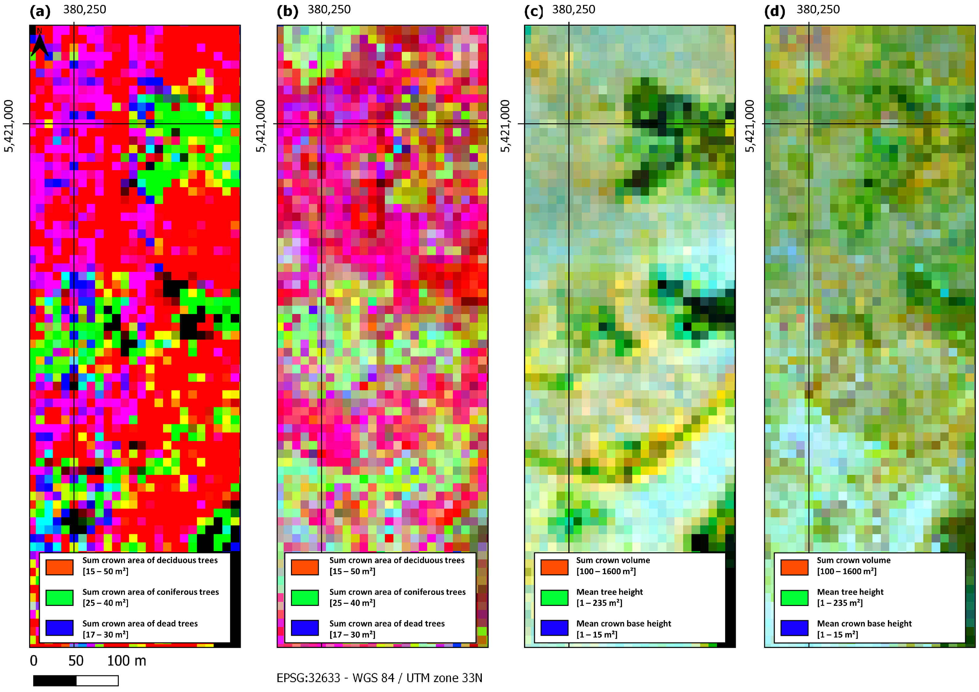
Table 1.
Characteristics of the examined areas of interest.
| AOI No. | Name | Rough Coordinates | Airborne Platform | Year | Area | No. of Trees |
|---|---|---|---|---|---|---|
| 1 | Steigerwald | 48°25′N, 11°40′E | Helicopter | 2017 | 2600 ha | 1,106,073 |
| 2 | Bavarian Forest National Park | 49°15′N, 13°15′E | Helicopter | 2016 | 1443 ha | 512,489 |
| 3 | Kranzberg Forest | 49°53′N, 10°32′E | UAV | 2020 | 7 ha | 1467 |
Table 2.
Rasterized single-tree polygon bands. The sum of the crown area might possibly exceed the pixel area because of overlays in tree canopy. To address these deficiencies, the proportion of tree canopy coverage per pixel is given as separate band. For lack of deadwood due to continuous forest management, the bands 3 and 6 may be completely zero in several study sites.
| Band | Variable | Unit | Value Range |
|---|---|---|---|
| 1 | Sum crown area of deciduous trees | m2 | 0–170 |
| 2 | Sum crown area of coniferous trees | m2 | 0–170 |
| 3 | Sum crown area of dead trees | m2 | 0–120 |
| 4 | Count of deciduous trees | amount | 0–9 |
| 5 | Count of coniferous trees | amount | 0–9 |
| 6 | Count of dead trees | amount | 0–7 |
| 7 | Tree area coverage | % | 0–100 |
| 8 | Sum crown volume | m3 | 0–3000 |
| 9 | Mean tree height | m | 0–43 |
| 10 | Mean crown base height | m | 0–24 |
Table 3.
Accuracy assessment of the random forest regression highlighting MAE, MAD, and STD per target value in the study site Steigerwald (AOI 1).
Table 3.
Accuracy assessment of the random forest regression highlighting MAE, MAD, and STD per target value in the study site Steigerwald (AOI 1).
| Variable | MAD | MAE | STD | Unit |
|---|---|---|---|---|
| Sum crown area of deciduous trees | 4.120 | 5.195 | 6.768 | m2 |
| Sum crown area of coniferous trees | 3.510 | 4.326 | 5.433 | m2 |
| Count of deciduous trees | 0.200 | 0.248 | 0.317 | amount |
| Count of coniferous trees | 0.090 | 0.133 | 0.193 | amount |
| Tree area coverage | 0.710 | 1.075 | 1.602 | % |
| Sum crown volume | 24.330 | 31.140 | 40.601 | m3 |
| Mean tree height | 0.709 | 0.962 | 1.220 | m |
| Mean crown base height | 0.430 | 0.530 | 0.692 | m |
Table 4.
Accuracy assessment of the random forest regression highlighting MAD, MAE, and STD per target value in the study site Bavarian Forest National Park (AOI 2).
Table 4.
Accuracy assessment of the random forest regression highlighting MAD, MAE, and STD per target value in the study site Bavarian Forest National Park (AOI 2).
| Variable | MAD | MAE | STD | Unit |
|---|---|---|---|---|
| Sum crown area of deciduous trees | 5.765 | 6.249 | 7.564 | m2 |
| Sum crown area of coniferous trees | 4.630 | 5.238 | 6.525 | m2 |
| Sum crown area of dead trees | 3.115 | 3.811 | 4.745 | m2 |
| Count of deciduous trees | 0.240 | 0.281 | 0.344 | amount |
| Count of coniferous trees | 0.190 | 0.221 | 0.262 | amount |
| Count of dead trees | 0.090 | 0.125 | 0.161 | amount |
| Tree area coverage | 1.345 | 2.133 | 3.202 | % |
| Sum crown volume | 52.130 | 64.858 | 83.534 | m3 |
| Mean tree height | 0.910 | 1.246 | 1.608 | m |
| Mean crown base height | 1.045 | 1.249 | 1.488 | m |
Table 5.
Accuracy assessment of the random forest regression highlighting MAE, MAD, and STD per target value in the study site Kranzberg Forest (AOI 3).
Table 5.
Accuracy assessment of the random forest regression highlighting MAE, MAD, and STD per target value in the study site Kranzberg Forest (AOI 3).
| Variable | MAD | MAE | STD | Unit |
|---|---|---|---|---|
| Sum crown area of deciduous trees | 7.800 | 6.917 | 7.513 | m2 |
| Sum crown area of coniferous trees | 4.700 | 6.759 | 8.663 | m2 |
| Count of deciduous trees | 0.170 | 0.156 | 0.186 | amount |
| Count of coniferous trees | 0.040 | 0.084 | 0.115 | amount |
| Tree area coverage | 1.320 | 2.955 | 5.423 | % |
| Sum crown volume | 117.410 | 140.235 | 134.399 | m3 |
| Mean tree height | 0.540 | 0.976 | 1.417 | m |
| Mean crown base height | 1.250 | 1.332 | 1.552 | m |
Disclaimer/Publisher’s Note: The statements, opinions and data contained in all publications are solely those of the individual author(s) and contributor(s) and not of MDPI and/or the editor(s). MDPI and/or the editor(s) disclaim responsibility for any injury to people or property resulting from any ideas, methods, instructions or products referred to in the content. |
© 2024 by the authors. Licensee MDPI, Basel, Switzerland. This article is an open access article distributed under the terms and conditions of the Creative Commons Attribution (CC BY) license (https://creativecommons.org/licenses/by/4.0/).
Share and Cite
MDPI and ACS Style
Hauser, S.; Ruhhammer, M.; Schmitt, A.; Krzystek, P. An Open Benchmark Dataset for Forest Characterization from Sentinel-1 and -2 Time Series. Remote Sens. 2024, 16, 488. https://doi.org/10.3390/rs16030488
AMA Style
Hauser S, Ruhhammer M, Schmitt A, Krzystek P. An Open Benchmark Dataset for Forest Characterization from Sentinel-1 and -2 Time Series. Remote Sensing. 2024; 16(3):488. https://doi.org/10.3390/rs16030488
Chicago/Turabian StyleHauser, Sarah, Michael Ruhhammer, Andreas Schmitt, and Peter Krzystek. 2024. "An Open Benchmark Dataset for Forest Characterization from Sentinel-1 and -2 Time Series" Remote Sensing 16, no. 3: 488. https://doi.org/10.3390/rs16030488
Note that from the first issue of 2016, this journal uses article numbers instead of page numbers. See further details here.