Edge Effects in Amazon Forests: Integrating Remote Sensing and Modelling to Assess Changes in Biomass and Productivity

Abstract

The tropical forests in the Amazon store large amounts of carbon and are still considered a carbon sink. There is evidence that deforestation can turn a forest landscape into a carbon source due to land use and forest degradation. Deforestation causes fragmented forest landscapes. It is known from field experiments that forest dynamics at the edge of forest fragments are altered by changes in the microclimate and increased tree mortality (“edge effects”). However, it is unclear how this will affect large fragmented forest landscapes, and thus the entire Amazon region. The aim of this study is to investigate different forest attributes in edge and core forest areas at high resolution, and thus to identify the large-scale impacts of small-scale edge effects. Therefore, a well-established framework combining forest modelling and lidar-generated forest structure information was combined with radar-based forest cover data. Furthermore, forests were also analyzed at the landscape level to investigate changes between highly fragmented and less-fragmented landscapes. This study found that the aboveground biomass in forest edge areas is 27% lower than in forest core areas. In contrast, the net primary productivity is 13% higher in forest edge areas than in forest core areas. In the second step, whole fragmented landscapes were analyzed. Nearly 30% of all forest landscapes are highly fragmented, particularly in the regions of the Arc of Deforestation, on the edge of the Andes and on the Amazon river banks. Less-fragmented landscapes are mainly located in the central Amazon rainforest. The aboveground biomass is 28% lower in highly fragmented forest landscapes than in less-fragmented landscapes. The net primary productivity is 13% higher in highly fragmented forest landscapes than in less-fragmented forest landscapes. In summary, fragmentation of the Amazon rainforest has an impact on forest attributes such as biomass and productivity, with mostly negative effects on forest dynamics. If deforestation continues and the proportion of highly fragmented forest landscapes increase, the effect may be even more intense. By combining lidar, radar and forest modelling, this study shows that it is possible to map forest structure, and thus the degree of forest degradation, over a large area and derive more detailed information about the carbon dynamics of the Amazon region.

1. Introduction

The Amazon rainforest is the largest intact tropical rainforest on Earth and stores a huge amount of carbon [1]. Yet, it is still considered a carbon sink [2,3], although first studies show a negative trend due to ongoing deforestation [3]. Deforestation not only leads to habitat loss and high carbon emissions, it also leads to a fragmented landscape of forests [4,5]. In South America, deforestation has been observed at a rate of 0.3% since 2000 [5,6,7]. Therefore, the forests in these fragmented landscapes are partially degraded [8]. The main cause of forest degradation is through forest edge effects driven by forest fragmentation [9]. The microclimate at the forest edge changes and thus forest dynamics are altered. The negative consequences of forest fragmentation in the first 100–300 m from the edge are losses in species diversity, increased tree mortality, less biomass and increased CO₂ emissions due to mortality and degradation [10,11,12].

Ongoing deforestation causes more forest edges, and therefore increased CO₂ emissions [1,4]. Model projections revealed that by 2100, 50% of the tropical forest area will be at the forest edge, resulting in additional carbon emissions of up to 500 million tons of carbon per year [5].

Since forest fragmentation has been accelerating for many decades, the edge effects should be visible in large parts of the Amazon. Previous studies estimated biomass changes in forests for the whole tropics at a coarse spatial resolution of 500 m [13]. They found that biomass was reduced in the first 500 m by ca. 25%. One explanation for this decline could be the changes in forest dynamics at forest edges, but this is difficult to assess due to the coarse resolution of the used satellite products.

To sum up, changes in the forest edges were observed either locally (with empirical data or lidar campaigns) or globally with low spatial resolution (500 m–1000 m). Since the forest edge effects only occur in a range of 100 m to 300 m, it is clear that a resolution of 500 m is not sufficient for such analysis. Furthermore, the use of passive optical satellite data are not necessarily appropriate for measurements in the dense vegetation of the Amazon and detecting forest degradation [14]. Active systems such as lidar are better suited for this, such as the lidar satellite mission GEDI [14].

By linking such lidar data with an individual-based forest model, various forest properties can be directly examined at the footprint level of the lidar measurement (here, 25 m), such as biomass and productivity [3,15,16]. In addition, radar measurements make it possible to distinguish between areas where the forest is currently still present and where the forest has previously been lost [17]. Such forest/non-forest maps (here from TanDEM-X with 50 m resolution) help to assess the current state of forest fragmentation [17]. By combining the radar-derived forest maps and high-resolution lidar remote sensing data with an individual-based forest model, the following questions can be answered:

(1) How does forest biomass and productivity differ in the edge and core area of forest stands throughout the whole Amazon?

(2) How strong is the effect of fragmentation on forest biomass and productivity for forest landscapes?

To answer these questions, the forest model FORMIND is used. Lidar data from the GEDI mission for the entire Amazon rainforest was integrated into this forest model. To determine the degree of fragmentation, we evaluated forest/non-forest maps from the TanDEM-X mission.

We suspect considerable differences in biomass and productivity depending on whether a forest stand is located on the edge or in the intact core area of a forest area. This should also lead to considerably lower biomass and productivity values in highly fragmented landscapes.

2. Materials and Methods

In this study, the lidar data from NASA’s Global Ecosystem Dynamics Investigation (GEDI) mission and radar data from DLR’s TanDEM-X mission were combined and integrated into the forest model FORMIND. The GEDI and FORMIND data fusion ensures the derivation of forest parameters (like biomass and productivity) through waveform matching. In addition, the TanDEM-X forest/non-forest data (50 m × 50 m) were used to investigate the state of forest fragmentation. By linking the derived forest parameters with the state of forest fragmentation, differentiated information on the forest parameters in forest edge areas and in forest core areas can be extracted and analyzed. It should be noted that the derivation of all forest parameters was performed at the GEDI footprint level (diameter of ~25 m) and the fragmentation state analysis at a resolution of 50 × 50 m. Only for the landscape analysis (see Section 3.3), for some visualization purposes, were these results aggregated at 100 km² areas.

2.1. Study Area

This study addressed an ecoregion of the Amazon rainforest with an area of 5.4 × 10⁶ km² and ranged from 10.5°N −80.0°W to −44.5°S −18.0°E. For the building of the mask for the Amazon ecoregion, the Ecoregion 2017 dataset was used [18].

2.2. Degree of Fragmentation from DLR TanDEM-X

The TerraSAR-X add-on for Digital Elevation (TanDEM-X) is a German radar satellite from the German Aerospace Center (DLR) and the first bistatic SAR mission. The aim of this mission was to generate a consistent global digital elevation model with high accuracy. TanDEM-X, launched in 2007, and TerraSAR-X, launched in 2010, were the first configurable Synthetic Aperture radars (SAR) in space. Both radar satellites moved around the Earth at an altitude of 500 km and flew in close formation [17,19].

For this study, data from the TanDEM-X global binary forest/non-forest Map (FNF), developed by the Microwaves and Radar Institute at the German Aerospace Center (DLR), were used [20]. The available data of TanDEM-X were captured between 2011 and 2016 using the stripmap single polarization (HH) mode of the TanDEM-X bistatic inerferometric synthetic aperture radar (InSAR) with a spatial resolution of 50 × 50 m and divided into 1° by 1° geocells. Pixels flagged as urban areas and invalid pixels were classified as non-forest [17,20].

To determine the distance of individual forest areas from the forest edge, the Hoshen–Kopelman algorithm was used [21]. This cluster detection algorithm has already been used in [4,5,22] for fragmentation analysis and forest edge detection. The connection between a forest pixel and forest in neighboring pixels was determined assuming a four-pixel neighborhood. An additional feature of this algorithm is that it determines the distance of each forest pixel to the nearest forest edge. This additional feature was already implemented and tested in [5]. These estimated distances make it possible to distinguish forest core areas from forest edge areas. Forest edge forest areas correspond to forest pixels with a distance of less than 100 m to the forest edge. If a non-forested area, e.g., a river or a road, is wider than 50 m, the neighboring forest borders are considered as edges. It should be noted that the algorithm cannot distinguish between anthropogenic and natural edges. The algorithm is implemented as a C++ program and calculates the distances as efficiently as possible. Further details of this forest fragmentation algorithm are explained in Fischer et al. 2021 [5].

2.3. Lidar Data from NASA GEDI

The Global Ecosystem Dynamics Investigation (GEDI) is a NASA mission that measures forest structure in temperate and tropical forests between 51.6° north and south. It is a large-footprint lidar system placed on the International Space Station (ISS) since 2018 and it generates waveforms and has a footprint diameter of ~25 m. The aim of this mission was to determine the effects of changing climate and land use on ecosystem structure and dynamics [14].

The GEDI laser system consists of three lasers: a coverage laser that is split into two lasers and two full power lasers that remain unchanged. The tracks are located within a ~4.2 km wide strip with a spacing of ~600 m and a footprint spacing per track of 60 m. The GEDI data consist of footprint and raster datasets and include information on the 3D characteristics of the vegetation. These data are associated with different levels of data processing. For this study, the Level2A data were used. These data contain ground height, canopy height and relative height percentiles (here a relative height of 95% (RH95) was used) [14].

For this study, data from 2019 to 2020 for the Amazon rainforest ecoregion were used. After filtering the data by quality flag and workflow processes about 110 million individual GEDI waveforms were available [3,23]. GEDI waveforms provide structure-based snapshots of aboveground biomass and forest productivity that can be decoded with the FORMIND forest model.

2.4. Individual-Based Forest Model FORMIND

FORMIND is an individual-based forest gap model developed in the late 1990s to simulate forest dynamics in high spatial resolution patches. In addition, physiological processes at the tree level were simulated [24,25,26,27,28]. The main processes of FORMIND are tree growth, tree mortality, recruitment and tree competition. In this study, we applied FORMIND to the tropical forest in the Amazon [15,26] where the parametrization was chosen as in Rödig et al. and Bauer et al. [3,15].

The forest model represents tree diversity by grouping tree species into three plant functional types (PFTs) [29] in the tradition of global vegetation models (PFT grouping from Rödig et al. [15,16,26] and Bauer et al. [3]). These three PFTs represent different successional stages: shade-intolerant pioneer species, shade-tolerant climax species and medium shade-tolerant tree species. It has been shown in several studies that this grouping could sufficiently describe forest dynamics and changes in species group compositions [15,26,30,31]. In addition, the parameters of the dominant PFT with the climax tree species were regionally adjusted. It was found that the mortality parameters of the forest model for shade-tolerant late-successional trees could be adjusted to better match forest inventory data and reproduce local measurements of aboveground forest biomass, mean wood density and basal area [26]. The regional mortality parameters depend on local characteristics such as climate conditions (e.g., precipitation) and soil properties (e.g., clay content), which were derived from global maps [26].

We then determined forest parameters like the aboveground biomass, net primary productivity, gross primary productivity and leaf area index of trees. In order to implement the FORMIND model for the complete Amazon rainforest, the Amazon was split into environmental regions and we performed forest simulations for the whole Amazon in high-resolution including simulations of lidar waveforms [26]. This well-established workflow, which combines FORMIND and GEDI data using waveform matching, determines the current forest condition in the Amazon region [3,16]. For the waveform matching (Figure 1), each real GEDI waveform was compared with hundreds of simulated lidar waveforms in the respective environmental region to determine the state of the forest. The simulated waveforms with the 50 best overlaps were used to determine the current forest condition because these waveforms matched best with the real GEDI data. Then, for the best matching forest stands it was possible to calculate forest attributes like the aboveground biomass, net ecosystem exchange, gross primary productivity, stem size distribution and leaf area index.

With this model-data fusion, we analyzed different forest properties at the footprint level of a GEDI shoot. The forest properties investigated were aboveground biomass (AGB in Mg organic dry mass (odm)), net primary productivity (NPP), gross primary productivity (GPP) and leaf area index (LAI). All attributes were calculated at the individual tree level and then summed up for all trees within the footprint. GPP is the sum of the gross primary productivities of all simulated trees within the footprint. NPP is the difference between GPP and maintenance respiration of trees. LAI is defined as the leaf area per ground surface (does not include grass and bushes).

2.5. Comparison with Other Satellite Data

In our model-data workflow, we derived the aboveground biomass and net primary productivity (NPP) values for the forests in the Amazon (among other things). We compared these values with maps from other sources: the aboveground biomass map for forests from Santoro et al. (radar remote sensing) [32] and the NPP map from MODIS (optical remote sensing) [33].

The aboveground biomass map contains data from 2018 with a resolution of 100 m. The NPP map from MODIS contains data from 2000 to 2010 with a resolution of approximately 1000 m. Both maps were adapted to the grid of the forest/non-forest map used in this study (50 m). This made it possible to distinguish the biomass and NPP values for the forest edge and core areas. We used R for the calculations.

3. Results

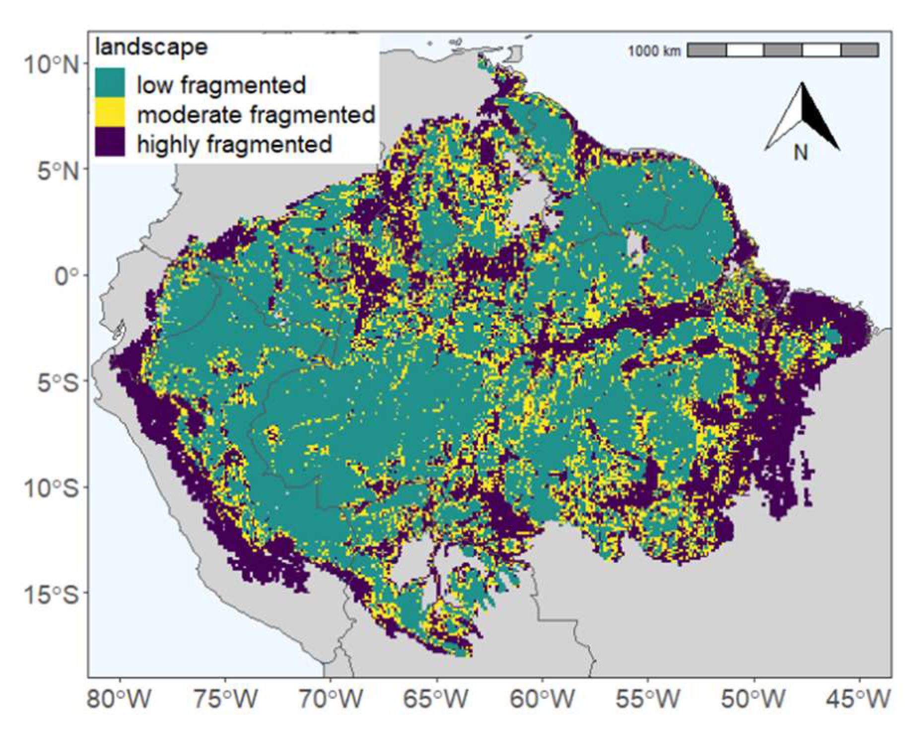
3.1. The Current State of Forest Distances in the Amazon

We analyzed more than 150 million lidar shots from the GEDI mission (25 m footprint) for the entire Amazon region and calculated the distance to the forest edge for each measurement using the TanDEM-X forest/non-forest map (50 m resolution X-band radar) (Figure 2a). The distances cover a range with values up to 42 km. On average, the distance from a forest stand to the edge is 1750 m (Figure 2c). The obtained distances to the forest edge in areas along the Amazon River, in the area of the Arc of Deforestation and near the Andes are rather small. Here, the distances of forests to non-forest areas range from 0 to 500 m. These values indicate a strong fragmentation of the rainforest. More intact areas with larger distances to the edge can be observed in central Amazon. Here, minor fragmentation has occurred and the distances to the nearest forest-free patch are at least 1500 m.

3.2. Impact of Forest Fragmentation on Amazon Rainforest at Forest Stand Level

Each GEDI shot was assigned to forest edge or forest core areas using the TanDEM-X forest/non-forest map. A forest edge is located up to 100 m away from non-forest areas and a forest core is located more than 100 m away from non-forest areas (Figure 3a). In this study, edge and core areas are distributed as follows: 6.5% of the Amazon is edge area and 93.5% is core area. Lidar waveform matching with a forest model provides important forest attributes (aboveground biomass AGB, net primary productivity NPP, gross primary productivity GPP and leaf area index LAI) for all GEDI shots (

Table 1. Mean values and standard deviation, the coefficient of variation (CV) for the four forest attributes considered: aboveground biomass, net primary productivity, gross primary productivity and leaf area index. In addition, the relative difference between the mean values of the edge and the mean values of the core area is given. The values were determined for the 110 million GEDI shots that lie in the edge and core area. CV is the ratio of the standard deviation to the mean.

	Edge (CV)	Core (CV)	Difference between Core and Edge Values
Aboveground biomass [Mg odm ha−1]	172 ± 86 (50%)	235 ± 85 (36%)	−27%
Net primary productivity [Mg C ha−1 a−1]	5.4 ± 1.5 (29%)	4.7 ± 1.3 (28%)	+13%
Gross primary productivity [Mg C ha−1 a−1]	22 ± 7 (31%)	24 ± 6 (23%)	−8%
Leaf area index [-]	3.9 ± 1.4 (35%)	4.6 ± 1.1 (25%)	−15%

, Figure 3 and Figure S2).

The mean value for AGB in the forest edge area is 172 ± 86 Mg odm ha⁻¹ compared to 235 ± 85 Mg odm ha⁻¹ in the core area. This means AGB is 37% higher in the forest core area than in the edge area. The coefficient of variation (CV) is 50% for the edge area and 36% for the core area, meaning higher AGB variability in the forest edge area than in the forest core area. (Table 1 and Figure 3a).

The NPP also shows different values for forest edge (mean: 5.4 ± 1.5 Mg C ha⁻¹ a⁻¹) and core (mean: 4.7 ± 1.3 Mg C ha⁻¹ a⁻¹) areas which differ by 13%. The distribution of NPP values in forest core areas is slightly narrower and thus less dispersed compared to NPP values in forest edge areas. It is noticeable that the CV of the two forest areas is similar (Figure 2c, Table 1).

In addition to AGB and NPP, the forest attributes GPP and NPP were also examined (Figure S2, Table 1). The obtained mean value for GPP in the forest edge area is 22 ± 7 Mg C ha⁻¹ a⁻¹ and 24 ± 6 Mg C ha⁻¹ a⁻¹ in the core area (Figure S2a, Table 1). For LAI, the mean value in the core is 18% larger than in the edge (Figure S2b, Table 1).

In addition to the analysis of forest stands, forest core areas were also investigated (Figures S3 and S4). Since no edge effects occur in the core area of forests, these AGB and NPP values should only depend on the site factors and not necessarily on fragmentation. We observe that low values of AGB dominate particularly in the areas of the Arc of Deforestation, on the edge of the Andes and on the Amazon River. Biomass values range from approx. 30–150 Mg odm ha⁻¹ and the net primary productivity values are between 1 and 3 Mg C ha⁻¹ a⁻¹.

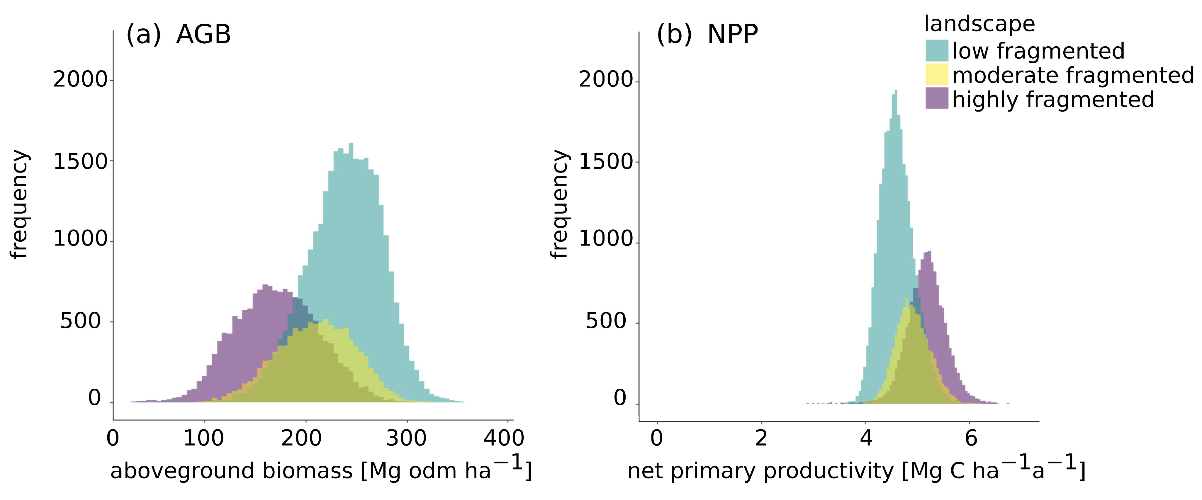
3.3. Impact of Forest Fragmentation on Amazon Biomass and Productivity at Landscape Level

In the first part of the study (Section 3.2), we analyzed the forest biomass and productivity on a fine scale (25 m). In most cases, only small differences were found between forest edge and core areas (e.g., for NPP +13%, for AGB −27%). In the second part of this study, we analyzed the impacts of fragmentation on forests on a landscape scale (10 × 10 km²). The classification of the landscape level was based on the degree of forest fragmentation. We divided the Amazon rainforest into three different classes: low-fragmented forest, moderate-fragmented forest and highly fragmented forest (Figure 4). Low-fragmented forest are regions in which less than 10% of the GEDI shots are in forest edge areas. Moderate-fragmented areas have between 10 and 25% edge area and highly fragmented areas are landscapes with more than 25% forest edge area. For the landscape analysis, this classification was used to differentiate between the various landscape types (Figure 4, Figure 5, Figure 6 and Figure 7).

The three different fragmentation landscape types are distributed as follows: 53.5% of the Amazon is low-fragmented, 18.3% moderate-fragmented and 28.2% highly fragmented (Figure 4). It is evident that low-fragmented landscapes dominate in the central Amazon. Highly fragmented landscapes are mainly found in the areas of the Arc of Deforestation, at the edge of the Andes and along the Amazon River. Moderate-fragmented landscapes are found in the transition zones.

The aboveground biomass, net primary productivity, gross primary productivity and leaf area index of forests were examined (10 × 10 km²). As a result, frequency distributions of the forest attributes were obtained (Figure 5 and Figure S7), including the respective mean values for low-fragmented, moderate-fragmented and highly fragmented areas.

The frequency distribution of the aboveground biomass (Figure 5a) shows a clear difference in the distributions for the three fragmentation landscape types with the highest values in low-fragmented landscapes. Low-fragmented areas show a mean of 238 Mg odm ha⁻¹, moderate-fragmented areas have a mean of 210 Mg odm ha⁻¹ and highly fragmented areas have a mean of 171 Mg odm ha⁻¹. For low-fragmented areas a lower standard deviation is observed than in highly fragmented areas. The CV for highly fragmented areas (24%) is 1.5 times greater than the CV for low-fragmented areas (16%).

For net primary productivity (Figure 5b), the mean values for all fragmentation types are quite similar (

Table 2. Mean values and standard deviations, as well as the coefficient of variation (CV) averaged within a 10 × 10 km² section for the four forest attributes considered: aboveground biomass, net primary productivity, gross primary productivity and leaf area index. Each fragment was assigned to a fragmentation landscape type based on the amount of edge area it contained: low-fragmented, moderate-fragmented and highly fragmented. CV is the ratio of the standard deviation to the mean.

	Highly Fragmented (CV)	Moderate Fragmented (CV)	Low Fragmented (CV)
Mean aboveground biomass [Mg odm ha−1]	171 ± 42 (24%)	210 ± 38 (18%)	238 ± 37 (16%)
Mean net primary productivity [Mg C ha−1 a−1]	5.2 ± 0.4 (7.6%)	4.9 ± 0.3 (6.7%)	4.6 ± 0.3 (7.2%)
Mean gross primary productivity [Mg C ha−1 a−1]	22 ± 3 (14%)	23 ± 2 (10%)	24 ± 2 (8%)
Mean leaf area index	3.8 ± 0.6 (16.3%)	4.3 ± 0.5 (12.5%)	4.6 ± 0.5 (11.2%)

). Highly fragmented areas have a mean value of 5.2 Mg C ha⁻¹ a⁻¹, moderate-fragmented areas a mean value of 4.9 Mg C ha⁻¹ a⁻¹ and low-fragmented areas a mean value of 4.6 Mg C ha⁻¹ a⁻¹. The mean value therefore increases with the degree of fragmentation.

For gross primary productivity, we observe slightly higher values in low-fragmented landscapes (Figure S7a and Table 2): 24 Mg C ha⁻¹ a⁻¹ for low-fragmented areas and 22 Mg C ha⁻¹ a⁻¹ for highly fragmented areas.

The mean values of the leaf area index are 4.6 for low-fragmented areas, 4.3 for moderate-fragmented areas and 3.8 for highly fragmented areas (Table 2, Figure S7b). The CV also increases for the areas with higher fragmentation.

We also analyzed how the biomass of core forest is influenced by fragmentation (of the landscape). The behavior of the biomass in the core area was then investigated with the percentage of edge per 100 km² tile (Figure 6). For landscapes with higher fragmentation, lower biomasses dominate, whereas for landscapes with a low edge proportion, core forests show high biomass. For edge percentages of 90–100%, the biomass values are between 80 and 180 Mg odm ha⁻¹, whereas the biomass for edge percentages of 0–10% is mainly between 130 and 350 Mg odm ha⁻¹. From this, we derive that for high biomass values core forests show a dependency on fragmentation (see also Section 4).

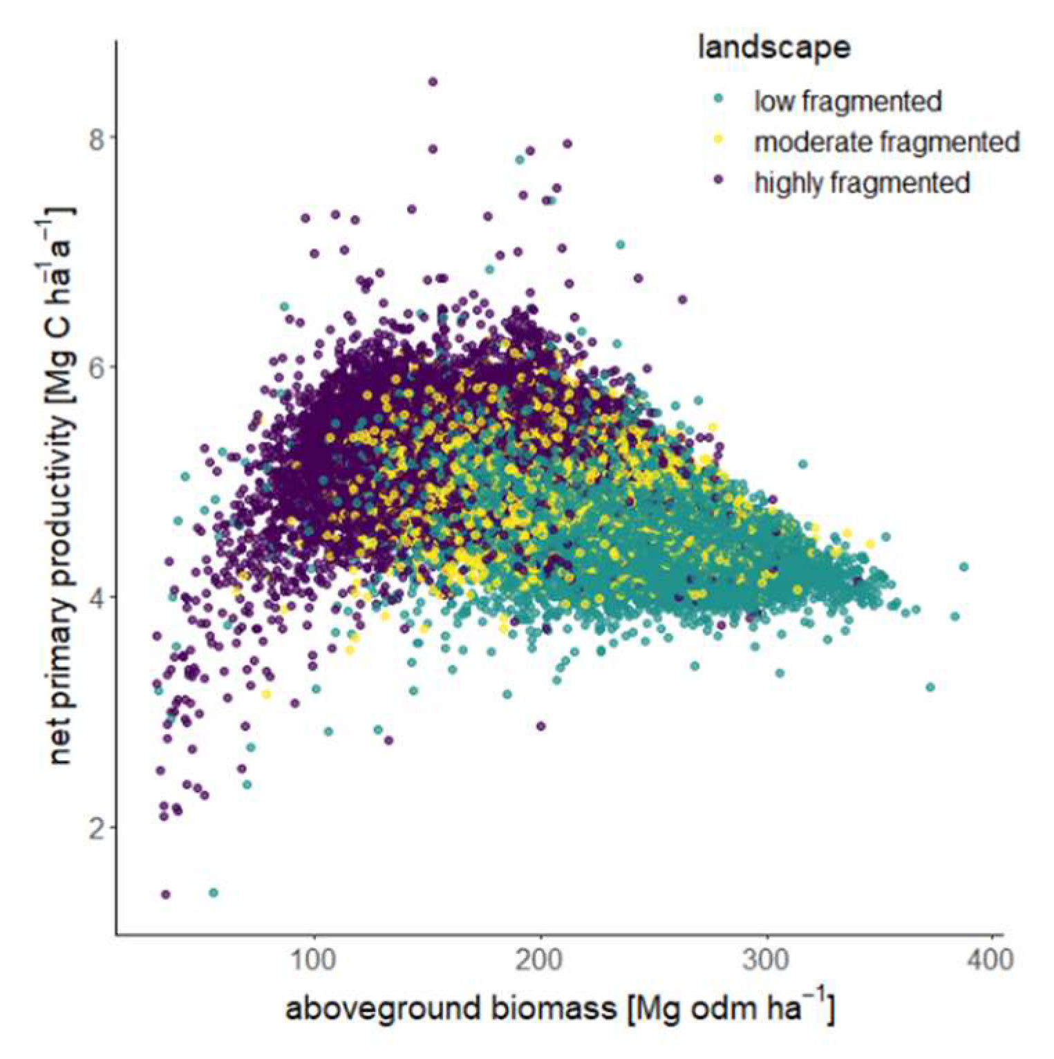
3.4. The Relationship between Forest Properties in Fragmented Landscapes

The relationship between aboveground biomass and productivity (Figure 7 and Figure S8) was investigated within 10 × 10 km² tiles. The tiles were assigned to the respective landscape classes according to the proportion of edge area.

This analysis shows two trends: on the one hand, an increasing NPP with increasing biomass and, on the other hand, a decreasing NPP with increasing biomass (Figure 7). For forest landscapes with low aboveground biomass (less than 150 Mg odm ha⁻¹), productivity increases from 3 to 6.5 Mg C ha⁻¹ a⁻¹ with increasing biomass. These landscapes are characterized by high fragmentation. The highest NPP values (around 6–7 Mg C ha⁻¹ a⁻¹) are obtained with a forest biomass in the landscape of around 150 Mg odm ha⁻¹. If the forest biomass is greater than 150 Mg odm ha⁻¹, the productivity is between 4 and 6 Mg C ha⁻¹ a⁻¹. Here, productivity decreases slightly with increasing biomass. Landscapes with a biomass greater than 150 Mg odm ha⁻¹ are characterized as moderate- or low-fragmented.

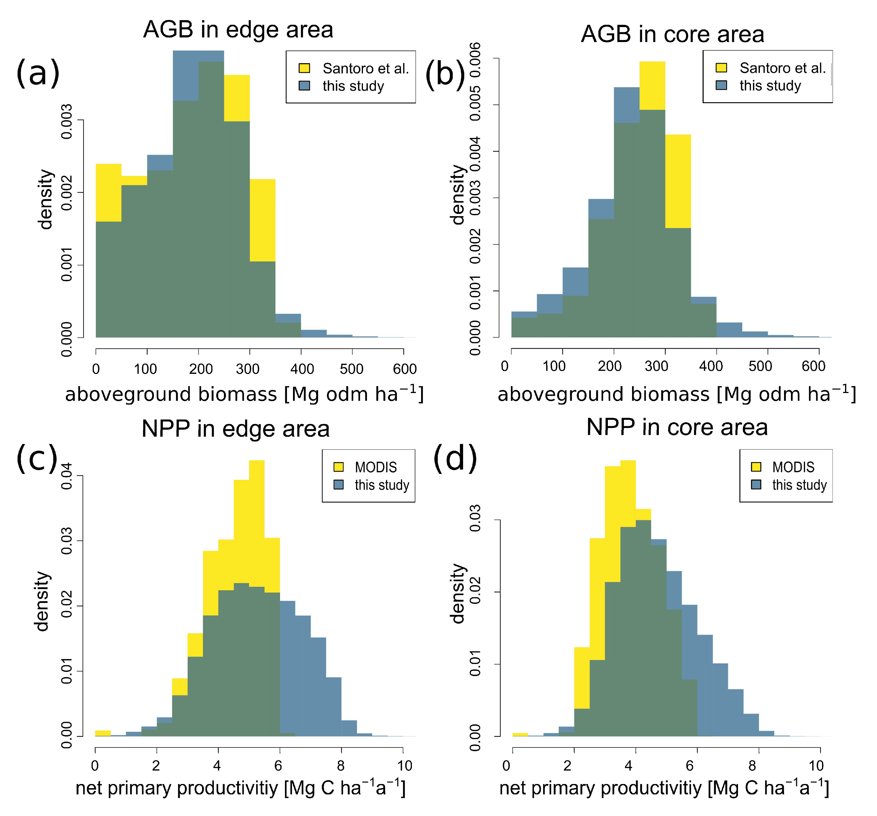
3.5. Comparison of Biomass and Productivity with Other Satellite Products

In our study, we found that differences in forest attributes depend on whether the forest was in an edge or core area. We observed a biomass of 172 Mg ha⁻¹ in the edge area, whereas it was 235 Mg ha⁻¹ in the core area (Table 1). This result is confirmed when the Santoro biomass map [32] is also divided into forest edge and core areas (Figure 8a,b). This analysis shows a clear agreement with our biomass estimations, as well as confirming the differences between the forest edge and core (Santoro: mean for forests at edge 186 Mg ha⁻¹; Santoro: mean for core forests 248 Mg ha⁻¹).

A similar comparison was made between the NPP values from MODIS. In general, for low and medium NPP values there is a good agreement between the NPP values estimated by MODIS and the method of this study (Figure 8c,d). Our NPP estimates tend to be slightly higher, which is mainly due to the fact that our workflow can detect structural changes in the forest, and thus also forest degradation. MODIS generally tends to produce lower NPP estimates, which has already been discussed in other studies [15,34].

In our study, we found that NPP is 5.4 Mg C ha⁻¹ a⁻¹ in the edge area and slightly lower at 4.7 C ha⁻¹ a⁻¹ in the forest core area (Table 1). Although MODIS provides overall lower NPP estimates, our observed trend is also confirmed by the MODIS measurements: the NPP from MODIS is 4.5 Mg C ha⁻¹ a⁻¹ for forest edges and 3.8 Mg C ha⁻¹ a⁻¹ for core forests.

4. Discussion

4.1. Summary

In this study, lidar data from the GEDI mission and radar data from the TanDEM-X mission were coupled with the simulations from a high-resolution forest model to obtain information on forest attributes and fragmentation states for forests in the Amazon. We found smaller differences in forest attributes at the forest stand level between the forest edge and forest core areas. At landscape level, larger differences in the forest attributes were observed for highly fragmented landscapes.

4.2. Impact of Fragmentation on Edge and Core Forests

In this study, differences in aboveground biomass, net primary productivity, gross primary productivity and leaf area index were analyzed between the edge and core areas (forest stand level). Except for net primary productivity, higher values were found in the core than in the edge forest areas. We assume that most of these observations result from edge effects. Edge effects occur due to an altered microclimate (e.g., wind or temperature), altered species composition or increased mortality in forests [10,11,12]. This leads to a reduction of biomass in forest edge areas. It is known that forest fragmentation also alters the dynamics in the edge area of forests [5,11,22,35,36,37,38]. Pütz et al. [1] found that the aboveground biomass in large fragments was reduced by up to 14.7%. For small fragments, the biomass was even reduced by 68.5%. In our study, the fragment sizes were not considered, but we obtained an average of 27% lower values for biomass in the edge areas than in the core areas. Chaplin–Kramer et al. [13] found that the biomass in the first 500 m of a forest fragment is on average 25% lower than in the forest core using optical satellite measurements (with limitation due to saturation effects).

Surprisingly, in our analysis, the net primary productivity in the edge area is 13% higher than in the core area, although the biomass is lower at the edge [39,40]. This can be explained, for example, by a change in species composition: productive pioneer species can dominate in the forest edge.

Please note that reductions in biomass and productivity depend not only on edge effects, but that there is also a history of fragmentation. It is often not known how long ago a deforestation event occurred. Depending on how long the edge effects have been acting, the differences in biomass can be larger or smaller. A decrease in biomass after deforestation can take up to 40–60 years [10]. The lidar measurements used in this study give us just one snapshot in time. In addition, other factors can influence the biomass or productivity at the edge of forests. These include, for example, site factors (such as climate and soil properties) or elevation (topology).

4.3. Fragmentation at the Landscape Scale

Since some questions remain unanswered in the footprint scale area, a larger scale was also analyzed. On the landscape scale, the proportion of the edge area compared to the total forest area of the landscape was analyzed as a measure of fragmentation state. We suspect that landscapes with a higher degree of fragmentation were deforested a longer time ago [41,42].

One result of our analysis shows that the gross primary productivity has lower values for highly fragmented landscapes in comparison with lower-fragmented landscapes. The results of net primary productivity at the landscape level are surprising because, in contrast to the GPP, it shows higher values in highly fragmented areas when compared with areas with a moderate or low fragmentation. There may be several reasons for this, but one main reason could be a different species composition in favor of fast-growing pioneer species. We also derived LAI values from the forest model. Typical values are in agreement with the MODIS measurements [43]. Please note, there could also be differences in LAI values. This is because the FORMIND forest model does not take into account the leaf area of shrubs or grasses, only the leaf area of trees. Please note, the workflow presented here has already been extensively tested for the Amazon against field data on forest biomass (114 plots, [16]) and against forest productivity (GPP and NPP from MODIS [3,16]). The quality of the used lidar simulator has been tested against field data from a large forest plot [16,44].

At the same time, it should be noted for the results at landscape level, that the recognizable differences between the fragmentation types are not only influenced by fragmentation itself, but regional effects can also have an influence. For example, forest biomass in the Andes is lower due to elevation and temperature. Biomass and productivity are also low in the Arc of Deforestation region because of the amount of deforestation that has occurred and is still occurring. Biomasses and productivities in the central Amazon are higher overall, as there is undisturbed rainforest here. Therefore, it would be interesting to analyze the results at landscape level in more detail in the future, as several factors may play a role in why we observe a low biomass and productivity in some areas (Figures S3 and S4). For follow-up studies, it would therefore be interesting to investigate the correlations with climate conditions (e.g., temperature and precipitation) and topological conditions (e.g., elevation) to analyze their effect on biomass differences.

4.4. Challenges in Combining Remote Sensing and Forest Models

There can be several reasons for challenges and uncertainties when combining different types of satellite data (here lidar and radar) with different resolutions and then integrating them into an individual-based forest model with its own resolution. Geolocation uncertainty can play a role especially when combining several data sources. The geolocation error of GEDI is approximately 10 m [14]. Because the GEDI measurements are merged with a forest cover map (resolution 50 m × 50 m) in this study, and the remaining analyses are performed at 1 km² or 100 km² resolution, we expect that a 10 m deviation has minor effects on the results.

It would also be interesting to analyze the temporal development of biomass and productivity in the forest stands. However, the period of the GEDI measurements is currently too short for this. In the coming years, it is planned that GEDI will continue to measure, which will allow us to further integrate data and expand our analysis.

For this study, the forest cover map from TanDEM-X was chosen. Please note, other forest cover maps are also available, such as the map from Hansen et al. [6]. Most of these forest cover maps are mainly based on passive optical satellite signals. These have their limitations for tropical forests, mainly due to frequent cloud cover. The advantage of the TanDEM-X map is that radar measurements are almost unaffected by cloud cover.

Smith et al. conducted a fragmentation study in the Amazon rainforest and found that reforestation with secondary forest could reduce the edge effects [45]. This study showed that the biomass in edge forest areas or highly fragmented forest areas is lower and reforestation of the affected areas would be useful to better protect the forest fragments from edge effects.

In summary, the validated workflow from Rödig et al. [16] and Bauer et al. [3] used for this study produced reasonable results and has the capability to transfer this model-data fusion to other continents (Africa and Asia). This could be used to investigate whether our results for the Amazon apply to other tropical regions.

5. Conclusions

In this study on fragmentation, forest modelling was combined with remote-sensing measurements (lidar, radar) to investigate the changes in forest attributes at the footprint and landscape scales. Changes in biomass and productivity were especially observed in highly fragmented landscapes. Biomass values are particularly high in low-fragmented areas, while the net primary productivity values are higher in highly fragmented areas. The study shows that a high degree of forest fragmentation should be avoided in order to maintain large continuous forest areas, and thus the carbon sequestration potential of forests.

References

1. Pütz, S.; Groeneveld, J.; Henle, K.; Knogge, C.; Martensen, A.C.; Metz, M.; Metzger, J.P.; Ribeiro, M.C.; Dantas de Paula, M.; Huth, A. Long-term carbon loss in fragmented Neotropical forests. Nat. Commun. 2014, 5, 5037. [Google Scholar] [CrossRef] [PubMed]
2. Gatti, L.V.; Gloor, M.; Miller, J.B.; Doughty, C.E.; Malhi, Y.; Domingues, L.G.; Basso, L.S.; Martinewski, A.; Correia, C.S.C.; Borges, V.F.; et al. Drought sensitivity of Amazonian carbon balance revealed by atmospheric measurements. Nature 2014, 506, 76–80. [Google Scholar] [CrossRef] [PubMed]
3. Bauer, L.; Knapp, N.; Fischer, R. Mapping Amazon forest productivity by fusing GEDI lidar waveforms with an individual-based forest model. Remote Sens. 2021, 13, 4540. [Google Scholar] [CrossRef]
4. Brinck, K.; Fischer, R.; Groeneveld, J.; Lehmann, S.; Dantas De Paula, M.; Pütz, S.; Sexton, J.O.; Song, D.X.; Huth, A. High resolution analysis of tropical forest fragmentation and its impact on the global carbon cycle. Nat. Commun. 2017, 8, 14855. [Google Scholar] [CrossRef] [PubMed]
5. Fischer, R.; Taubert, F.; Müller, M.S.; Groeneveld, J.; Lehmann, S.; Wiegand, T.; Huth, A. Accelerated forest fragmentation leads to critical increase in tropical forest edge area. Sci. Adv. 2021, 7, eabg7012. [Google Scholar] [CrossRef] [PubMed]
6. Hansen, M.C.; Potapov, P.V.; Moore, R.; Hancher, M.; Turubanova, S.A.; Tyukavina, A.; Thau, D.; Stehman, S.V.; Goetz, S.J.; Loveland, T.R.; et al. High-resolution global maps of 21st-century forest cover change. Science 2013, 342, 850–853. [Google Scholar] [CrossRef] [PubMed]
7. Houghton, R.A.; Skole, D.L.; Nobre, C.A.; Hackler, J.L.; Lawrence, K.T.; Chomentowski, W.H. Annual fluxes or carbon from deforestation and regrowth in the Brazilian Amazon. Nature 2000, 403, 301–304. [Google Scholar] [CrossRef] [PubMed]
8. Lapola, D.M.; Pinho, P.; Barlow, J.; Aragão, L.E.O.C.; Berenguer, E.; Carmenta, R.; Liddy, H.M.; Seixas, H.; Silva, C.V.J.; Silva-Junior, C.H.L.; et al. The drivers and impacts of Amazon forest degradation. Science 2023, 379, eabp8622. [Google Scholar] [CrossRef]
9. Numata, I.; Cochrane, M.A.; Souza, C.M.; Sales, M.H. Carbon emissions from deforestation and forest fragmentation in the Brazilian Amazon. Environ. Res. Lett. 2011, 6, 044003. [Google Scholar] [CrossRef]
10. Laurance, W.F.; Camargo, J.L.C.; Luizao, R.C.C.; Laurance, S.G.; Pimm, S.L.; Bruna, E.M.; Stouffer, P.C.; Williamson, G.B.; Benitez-Malvido, J.; Vasconcelos, H.L.; et al. The fate of Amazonian forest fragments: A 32-year investigation. Biol. Conserv. 2011, 144, 56–67. [Google Scholar] [CrossRef]
11. Qie, L.; Lewis, S.L.; Sullivan, M.J.P.; Lopez-Gonzalez, G.; Pickavance, G.C.; Sunderland, T.; Ashton, P.; Hubau, W.; Abu Salim, K.; Aiba, S.-I.; et al. Long-term carbon sink in Borneo’s forests halted by drought and vulnerable to edge effects. Nat. Commun. 2017, 8, 1966. [Google Scholar] [CrossRef] [PubMed]
12. Laurance, W.F.; Camargo, J.L.C.; Fearnside, P.M.; Lovejoy, T.E.; Williamson, G.B.; Mesquita, R.C.G.; Meyer, C.F.J.; Bobrowiec, P.E.D.; Laurance, S.G.W. An Amazonian rainforest and its fragments as a laboratory of global change. Biol. Rev. 2018, 93, 223–247. [Google Scholar] [CrossRef] [PubMed]
13. Chaplin-Kramer, R.; Ramler, I.; Sharp, R.; Haddad, N.M.; Gerber, J.S.; West, P.C.; Mandle, L.; Engstrom, P.; Baccini, A.; Sim, S.; et al. Degradation in carbon stocks near tropical forest edges. Nat. Commun. 2015, 6, 10158. [Google Scholar] [CrossRef] [PubMed]
14. Dubayah, R.; Blair, J.B.; Goetz, S.; Fatoyinbo, L.; Hansen, M.; Healey, S.; Hofton, M.; Hurtt, G.; Kellner, J.; Luthcke, S.; et al. The Global Ecosystem Dynamics Investigation: High-resolution laser ranging of the Earth’s forests and topography. Sci. Remote Sens. 2020, 1, 100002. [Google Scholar] [CrossRef]
15. Rödig, E.; Cuntz, M.; Rammig, A.; Fischer, R.; Taubert, F.; Huth, A. The importance of forest structure for carbon fluxes of the Amazon rainforest. Environ. Res. Lett. 2018, 13, 054013. [Google Scholar] [CrossRef]
16. Rödig, E.; Knapp, N.; Fischer, R.; Bohn, F.J.; Dubayah, R.; Tang, H.; Huth, A. From small-scale forest structure to Amazon-wide carbon estimates. Nat. Commun. 2019, 10, 5088. [Google Scholar] [CrossRef] [PubMed]
17. Martone, M.; Rizzoli, P.; Wecklich, C.; González, C.; Bueso-Bello, J.-L.; Valdo, P.; Schulze, D.; Zink, M.; Krieger, G.; Moreira, A. The global forest/non-forest map from TanDEM-X interferometric SAR data. Remote Sens. Environ. 2018, 205, 352–373. [Google Scholar] [CrossRef]
18. Dinerstein, E.; Olson, D.; Joshi, A.; Vynne, C.; Burgess, N.D.; Wikramanayake, E.; Hahn, N.; Palminteri, S.; Hedao, P.; Noss, R.; et al. An ecoregion-based approach to protecting half the terrestrial realm. BioScience 2017, 67, 534–545. [Google Scholar] [CrossRef]
19. Krieger, G.; Moreira, A.; Fiedler, H.; Hajnsek, I.; Werner, M.; Younis, M.; Zink, M. TanDEM-X: A satellite formation for high-resolution SAR interferometry. IEEE Trans. Geosci. Remote Sens. 2007, 45, 3317–3341. [Google Scholar] [CrossRef]
20. Bueso Bello, J.L.; González, C.; Martone, M.; Rizzoli, P. TanDEM-X Forest/Non-Forest Map Product Description; DLR Microwaves and Radar Institute: Köln, Germany, 2019. [Google Scholar]
21. Hoshen, J.; Klymko, P.; Kopelman, R. Percolation and cluster distribution. III. Algorithms for the site-bond problem. J. Stat. Phys. 1979, 21, 583–600. [Google Scholar] [CrossRef]
22. Taubert, F.; Fischer, R.; Groeneveld, J.; Lehmann, S.; Müller, M.S.; Rödig, E.; Wiegand, T.; Huth, A. Global patterns of tropical forest fragmentation. Nature 2018, 554, 519–522. [Google Scholar] [CrossRef] [PubMed]
23. Beck, J.; Wirt, B.; Armston, J.; Hofton, M.; Luthke, S.; Tang, H. GLOBAL Ecosystem Dynamics Investigation (GEDI) Level 2 User Guide for SDPS PGEVersion 3 (P003) of GEDI L2A Data and SDPS PGEVersion 3 (P003) of GEDI L2B Data Version 2.0 April 2021; GEDI Ecosystem Lidar: Reston, VA, USA, 2021; p. 25. [Google Scholar]
24. Fischer, R.; Bohn, F.; Dantas de Paula, M.; Dislich, C.; Groeneveld, J.; Gutiérrez, A.G.; Kazmierczak, M.; Knapp, N.; Lehmann, S.; Paulick, S.; et al. Lessons learned from applying a forest gap model to understand ecosystem and carbon dynamics of complex tropical forests. Ecol. Model. 2016, 326, 124–133. [Google Scholar] [CrossRef]
25. Köhler, P.; Huth, A. The effects of tree species grouping in tropical rainforest modelling: Simulations with the individual-based model FORMIND. Ecol. Model. 1998, 109, 301–321. [Google Scholar] [CrossRef]
26. Rödig, E.; Cuntz, M.; Heinke, J.; Rammig, A.; Huth, A. Spatial heterogeneity of biomass and forest structure of the Amazon rain forest: Linking remote sensing, forest modelling and field inventory. Glob. Ecol. Biogeogr. 2017, 26, 1292–1302. [Google Scholar] [CrossRef]
27. Bohn, F.J.; Frank, K.; Huth, A. Of climate and its resulting tree growth: Simulating the productivity of temperate forests. Ecol. Model. 2014, 278, 9–17. [Google Scholar] [CrossRef]
28. Henniger, H.; Huth, A.; Frank, K.; Bohn, F.J. Creating virtual forests around the globe and analysing their state space. Ecol. Model. 2023, 483, 110404. [Google Scholar] [CrossRef]
29. Smith, T.M.; Shugart, H.H.; Woodward, F.I.; Burton, P.J. Plant functional types. In Vegetation Dynamics & Global Change; Springer: Boston, MA, USA, 1993; pp. 272–292. [Google Scholar]
30. Fischer, R.; Rödig, E.; Huth, A. Consequences of a reduced number of plant functional types for the simulation of forest productivity. Forests 2018, 9, 460. [Google Scholar] [CrossRef]
31. Fischer, R.; Knapp, N.; Bohn, F.; Shugart, H.H.; Huth, A. The relevance of forest structure for biomass and productivity in temperate forests: New perspectives for remote sensing. Surv. Geophys. 2019, 40, 709–734. [Google Scholar] [CrossRef]
32. Santoro, M.; Cartus, O.; Carvalhais, N.; Rozendaal, D.M.A.; Avitabile, V.; Araza, A.; de Bruin, S.; Herold, M.; Quegan, S.; Rodríguez-Veiga, P.; et al. The global forest above-ground biomass pool for 2010 estimated from high-resolution satellite observations. Earth Syst. Sci. Data 2021, 13, 3927–3950. [Google Scholar] [CrossRef]
33. Zhao, M.; Running, S.; Heinsch, F.A.; Nemani, R. MODIS-derived terrestrial primary production. In Land Remote Sensing and Global Environmental Change; NASA’s Earth observing system and the science of ASTER and MODIS; Springer: New York, NY, USA, 2011; pp. 635–660. [Google Scholar]
34. Park, J.H.; Gan, J.; Park, C. Discrepancies between global forest net primary productivity estimates derived from MODIS and forest inventory data and underlying factors. Remote Sens. 2021, 13, 1441. [Google Scholar] [CrossRef]
35. Laurance, W.F.; Bierregaard, R.O. (Eds.) Tropical Forest Remnants. Ecology, Management, and Conservation of Fragmented Communities; Cambridge University Press: Chicago, IL, USA, 1997; p. 616. [Google Scholar]
36. Laurance, W.F.; Delamonica, P.; Laurance, S.G.; Vasconcelos, H.L.; Lovejoy, T.E. Conservation—Rainforest fragmentation kills big trees. Nature 2000, 404, 836. [Google Scholar] [CrossRef] [PubMed]
37. Nunes, M.H.; Vaz, M.C.; Camargo, J.L.C.; Laurance, W.F.; de Andrade, A.; Vicentini, A.; Laurance, S.; Raumonen, P.; Jackson, T.; Zuquim, G.; et al. Edge effects on tree architecture exacerbate biomass loss of fragmented Amazonian forests. Nat. Commun. 2023, 14, 8129. [Google Scholar] [CrossRef] [PubMed]
38. Haddad, N.M.; Brudvig, L.A.; Clobert, J.; Davies, K.F.; Gonzalez, A.; Holt, R.D.; Lovejoy, T.E.; Sexton, J.O.; Austin, M.P.; Collins, C.D.; et al. Habitat fragmentation and its lasting impact on Earth’s ecosystems. Sci. Adv. 2015, 1, e1500052. [Google Scholar] [CrossRef]
39. Laurance, W.F.; Nascimento, H.E.M.; Laurance, S.G.; Andrade, A.C.A.; Fearnside, P.M.; Ribeiro, J.E.L.; Capretz, R.L. Rain forest fragmentation and the proliferation of successional trees. Ecology 2006, 87, 469–482. [Google Scholar] [CrossRef]
40. Laurance, W.F. Hyperdynamism in fragmented habitats. J. Veg. Sci. 2002, 13, 595–602. [Google Scholar] [CrossRef]
41. Ewers, R.M.; Didham, R.K.; Pearse, W.D.; Lefebvre, V.; Rosa, I.M.D.; Carreiras, J.M.B.; Lucas, R.M.; Reuman, D.C. Using landscape history to predict biodiversity patterns in fragmented landscapes. Ecol. Lett. 2013, 16, 1221–1233. [Google Scholar] [CrossRef] [PubMed]
42. Numata, I.; Silva, S.S.; Cochrane, M.A.; d’Oliveira, M.V.N. Fire and edge effects in a fragmented tropical forest landscape in the southwestern Amazon. For. Ecol. Manag. 2017, 401, 135–146. [Google Scholar] [CrossRef]
43. Caldararu, S.; Palmer, P.I.; Purves, D.W. Inferring Amazon leaf demography from satellite observations of leaf area index. Biogeosciences 2012, 9, 1389–1404. [Google Scholar] [CrossRef]
44. Knapp, N.; Huth, A.; Kugler, F.; Papathanassiou, K.; Condit, R.; Hubbell, S.P.; Fischer, R. Model-assisted estimation of tropical forest biomass change: A comparison of approaches. Remote Sens. 2018, 10, 731. [Google Scholar] [CrossRef]
45. Smith, C.C.; Barlow, J.; Healey, J.R.; de Sousa Miranda, L.; Young, P.J.; Schwartz, N.B. Amazonian secondary forests are greatly reducing fragmentation and edge exposure in old-growth forests. Environ. Res. Lett. 2023, 18, 124016. [Google Scholar] [CrossRef]
Figure 1. A lidar profile from the GEDI mission (blue) is compared with hundreds of simulated lidar profiles derived from a forest model (red). The forest model simulates site-specific forest dynamics and the corresponding lidar profile for each simulated forest stand. The real GEDI lidar measurements act as a filter to select the current forest state from all possible forest states. More details on this approach can be found in [3,16].
Remotesensing 16 00501 g001
Figure 2. The Distance map of the Amazon rainforest is shown in (a). The distance map indicates the distance of each forest stand to the nearest forest edge. For visualization purposes the scale is limited to 1500 m distance. The map has a resolution of 1 km2, also the analysis was performed at 50 m resolution. In addition, a zoomed-in section of a selected region is shown. In (b), the TanDEM-X forest/non-forest map with a resolution of 50 m, as well as the GEDI footprints (grey) available in this area (here: approx. 190,000 shots) and a part of the Amazon river (black) is shown. In (c), the histogram corresponding to (a) with a resolution of 1 km2 is shown. The mean value of the average distances to the forest edge is shown in red at 1750 m. The maximum value of the mean distance to the forest edge in the Amazon is 42 km. A histogram corresponding to (a) on footprint level can be found in the attachment (Figure S1).
Remotesensing 16 00501 g002
Figure 3. The density distribution of aboveground biomass (b) and net primary productivity (c) for edge and core areas. Core and edge areas are defined as in the scheme shown in (a). Non-forest is at 0 m, edge ranges from 0 to 100 m distance from non-forest and core areas are at >100 m distance from non-forest areas. In the density plots, the mean value of aboveground biomass and net primary productivity is shown accordingly in the coloring of edge and core. The relative frequency was plotted for all 110 million GEDI shots for the respective forest attributes at footprint level.
Remotesensing 16 00501 g003
Figure 4. The Amazon map divided into three regions: low-fragmented (petrol blue), moderate-fragmented (yellow) and highly fragmented (purple). In each 10 km2 cell, the GEDI shots were counted and then the percentage of edge regions was calculated. If less than 10% of the GEDI shots in the considered tile are in the edge region, it is a low-fragmented area, tiles with an edge percentage between 10% and 25% are assigned as moderate-fragmented areas, and regions with more than 25% edge region are highly fragmented. A map showing the Amazon-wide values of edge proportions can be found in the attachment (Figure S6).
Remotesensing 16 00501 g004
Figure 5. The frequency distribution for the mean aboveground biomass (a) and net primary productivity (b) within a 10 × 10 km2 tile, divided according to fragmentation landscape classes (low-fragmented, moderate-fragmented and highly fragmented).
Remotesensing 16 00501 g005
Figure 6. A Scatterplot showing the amount of forest edge area in a forested landscape against the aboveground biomass of forest core area in this landscape. The proportion was calculated by dividing the area of edge forest by the total forest area in a landscape. One pixel corresponds to a 100 km2 tile in the Amazon. Note that the vertical lines at 0%, 50% and 100% result from the landscape pixels with a sparse amount of forest, and thus a low number of lidar measurements (<20 GEDI shots per 100 km2). Typically, a 100 km2 landscape pixel has about 2000 lidar measurements. The vertical lines at 0% and 100% correspond to landscape pixels in which there are only core areas (0% fraction of forest edge area) or only edge areas (100% fraction of forest edge area).
Remotesensing 16 00501 g006
Figure 7. Scatterplot showing the relationship between the aboveground biomass and net primary productivity. Each point represents a 10 × 10 km2 section in which the GEDI shots and the associated forest attributes were averaged and assigned to the fragmentation landscape types (low-fragmented, moderate-fragmented and highly fragmented) based on their edge proportion.
Remotesensing 16 00501 g007
Figure 8. Comparison between the results of this study and other satellite data. Aboveground biomass (AGB; a,b) and net primary productivity (NPP; c,d) were compared for forests in the Amazon (frequency distribution, resolution for biomass 100 m × 100 m, for NPP 1000 m × 1000 m). A distinction was made between the values in the forest edge area (left) and in the core area (right). The biomass values of this study were compared with the biomass values of Santoro et al. [32], NPP estimates with the NPP values derived from MODIS satellite [33].
Remotesensing 16 00501 g008