Article

Using Remote Sensing Multispectral Imagery for Invasive Species Quantification: The Effect of Image Resolution on Area and Biomass Estimation

by
Manuel de Figueiredo Meyer
1,
José Alberto Gonçalves
1,2 and
Ana Maria Ferreira Bio
1,*
1
Interdisciplinary Centre of Marine and Environmental Research (CIIMAR/CIMAR), University of Porto, 4099-002 Porto, Portugal
2
Department of Geosciences Environment and Spatial Planning, Faculty of Sciences, University of Porto, 4169-007 Porto, Portugal
*
Author to whom correspondence should be addressed.
Remote Sens. 2024, 16(4), 652; https://doi.org/10.3390/rs16040652
Submission received: 23 December 2023 / Revised: 1 February 2024 / Accepted: 6 February 2024 / Published: 9 February 2024
(This article belongs to the Special Issue Remote Sensing for 2D/3D Mapping)

Abstract

:
This study assesses the applicability of different-resolution multispectral remote sensing images for mapping and estimating the aboveground biomass (AGB) of Carpobrotus edulis, a prominent invasive species in European coastal areas. This study was carried out on the Cávado estuary sand spit (Portugal). The performance of three sets of multispectral images with different Ground Sample Distances (GSDs) were compared: 2.5 cm, 5 cm, and 10 cm. The images were classified using the supervised classification algorithm random forest and later improved by applying a sieve filter. Samples of C. edulis were also collected, dried, and weighed to estimate the AGB using the relationship between the dry weight (DW) and vegetation indices (VIs). The resulting regression models were evaluated based on their coefficient of determination (R2), Normalised Root Mean Square Error (NRMSE), p-value, Akaike information criterion (AIC), and the Bayesian information criterion (BIC). The results show that the three tested image resolutions allow for constructing reliable coverage maps of C. edulis, with overall accuracy values of 89%, 85%, and 88% for the classification of the 2.5 cm, 5 cm, and 10 cm GSD images, respectively. The best-performing VI-DW regression models achieved R2 = 0.87 and NRMSE = 0.09 for the 2.5 cm resolution; R2 = 0.77 and NRMSE = 0.12 for the 5 cm resolution; and R2 = 0.64 and NRMSE = 0.15 for the 10 cm resolution. The C. edulis area and total AGB were 3441.10 m2 and 28,327.1 kg (with an AGB relative error (RE) = 0.08) for the 2.5 cm resolution; 3070.04 m2 and 29,170.8 kg (AGB RE = 0.08) for the 5 cm resolution; and 2305.06 m2 and 22,135.7 kg (AGB RE = 0.11) for the 10 cm resolution. Spatial and model differences were analysed in detail to determine their causes. Final analyses suggest that multispectral imagery of up to 5 cm GSD is adequate for estimating C. edulis distribution and biomass.

1. Introduction

In the ever-evolving field of remote sensing (RS), the selection of the appropriate scale to investigate an object plays a central role in the accuracy and relevance of information, as geographical phenomena, distributions, and processes are generally scale-dependent [1]. As new sensors and platforms are developed through new technological advancements, from aeroplanes to drones as observation platforms, from panchromatic to hyperspectral sensors, the overall effectiveness of an RS study is still strongly related to its images’ Ground Sample Distance (GSD). There is, however, a trade-off between the efficiency (extension of the area covered per survey) and spatial resolution, which are usually inversely proportional, with higher spatial resolutions linked to smaller areas covered.
Many studies use data collected from small areas obtained with high spatial resolution sensors to extrapolate their findings to more extensive areas surveyed with lower spatial resolution sensors [2,3,4]. Even though good results can be achieved this way, these studies do not consider the scale effect. In other words, these studies often neglect to address that, for a specific area and object of study, there is an optimal monitoring scale [5].
The investigation of optimal resolutions and the impact of spatial resolution on a land cover classification map (scale effect) has been the object of study of many articles [6,7,8,9,10,11,12,13,14]. These studies can be divided into two main types: those that use very high spatial resolution images and resample the images to simulate lower resolutions [7,8,11], and studies that use different equipment with different spatial resolutions [6,9,10,12,13]. Both approaches can produce interesting insights about the comparison of resolutions for a determined study objective. The present study uses the second approach, employing a UAV and an aeroplane platform equipped with multispectral cameras. This approach was selected considering the scope of this study, which is to assist in the selection of the means and methods for monitoring C. edulis.
Remote sensing techniques constitute a valuable tool for the management of invasive species. Unoccupied aerial vehicles (UAVs) equipped with multispectral sensors have been increasingly used to identify and monitor different invasive species in many ecosystems, and their application can be considered a well-established technique [15,16,17]. Additionally, multispectral UAVs have also gained importance in commercial agriculture, where vegetation indices (VIs) are used for crop health assessment and yield estimation [18,19,20]. Some recent studies of natural habitats have combined a species identification methodology with yield estimations to assess the vegetation’s aboveground biomass (AGB) using multi- or hyperspectral UAVs [21,22]. The measurement of the AGB of invasive species can play a central role in the planning and execution of vegetation management campaigns.
Originally from South Africa, Carpobrotus edulis is a prominent invasive species in Europe, with its genus Carpobrotus having the largest number of records of control actions in Mediterranean countries [23]. Remote sensing methods are an obvious choice to facilitate Carpobrotus monitoring and management. The objective of the present work was to evaluate the impact of remote sensing image resolution on C. edulis AGB estimation. Three sets of multispectral images with different spatial resolutions (2.5 cm, 5 cm, and 10 cm GSD) were examined, specifically focusing on each resolution’s accuracy in estimating C. edulis AGB. The results were compared to evaluate the most suitable resolution for C. edulis monitoring. Data processing, classification algorithms, and the subsequent implications for AGB estimate accuracies were evaluated to gain insights into the resolution impacts and improve the decision-making process on monitoring and removal campaigns.

2. Study Area

The study area was part of the Parque Natural do Litoral Norte (PNLN), administered by the national Nature and Forest Conservation Institute (Instituto da Conservação da Natureza e das Florestas–ICNF) (Figure 1). The park spreads along 16 km of the coast, located between the Neiva estuary (41°36′46.56″N, 8°48′32.55″W) and the south border of Apúlia (41°28′10.68″N, 8°46′31.30″W), extending 5 km offshore into the ocean. It covers a total of 8887 ha, of which 7653 ha are marine areas.
The PNLN was created to protect the littoral of Esposende, preserve its natural resources and elements, and promote a rational use of the site. With its mainland consisting essentially of a strip of sandy shores, the park houses 15 different habitats described in the Habitat Directive, 4 of which are marked as priority habitats: 1150-Coastal lagoons, 2130-Fixed coastal dunes with herbaceous vegetation (grey dunes), 2270-Wooded dunes with Pinus pinea and/or Pinus pinaster, and 91E0-Alluvial forests with Alnus glutinosa and Fraxinus excelsior (Alno-Padion, Alnion incanae, Salicion albae).
Almost all in-land park terrain is located less than 10 m above mean sea level, with only some dunes between 10 and 20 m high. There are 240 different vegetation species identified on the NLNP, most of them native to the north Iberic littoral, including some endangered species. This native vegetation is vital for preserving the morphological and biotic characteristics of the ecosystems [24]. However, like many other coastal environments, the dunes of the Cávado Estuary suffer not only from erosion risks but also from the constant pressure of climate change, urbanisation, recreation trampling, and invasive species [25]. Twelve invasive species were identified within the flora, with the most prominent ones considered the Acacia longifolia and Carpobrotus edulis, which pose significant pressure on the dune habitats [26].

3. Materials and Methods

This study was divided into four phases: in situ work (Section 3.1), laboratory work (Section 3.2), imagery processing (Section 3.3), and C. edulis area and biomass estimation (Section 3.4) (the methodology follows [27]).

3.1. In Situ Work

The in situ work was developed as follows: (i) marking of ground control points, (ii) placement of quadrats for sampling delimitation, and (iii) capture of aerial images.

3.1.1. Ground Control Points

Ground control points (GCPs) were strategically distributed over the study area and marked with spray paint. These points were georeferenced with a GNSS receiver Emlid Reach M2 and a NovAtel antenna GPS-702-GG (NovAtel—Calgary, AB, Canada) in Real-Time Kinematic (RTK) mode, with corrections from the National Network of Permanent Stations (ReNEP), the Portuguese CORS (Continuously Operating Reference Station) network, and later used to enhance the orthomosaic geometry and geolocation precision during imagery processing.

3.1.2. Sample Quadrats

Thirty 50 × 50 cm2 quadrats were placed over areas exclusively covered by C. edulis vegetation, each exhibiting distinct visually identified biomass and health characteristics (Figure 2a). This distribution was designed to cover a range of conditions, with more or less lush plants and different biomasses per sample, to optimise the dry weight (DW)–vegetation indices (VIs) regression models. The quadrats were placed with a north–south orientation, which helps to reduce the number of pixels the frames occupy in the RS image and the number of neighbouring pixels that are affected by interference on reflectance from the frame.
These quadrats have an essential role in identifying the sample areas. As they can be identified in the aerial images, they are used as visual marks for the samples. Their north-west and south-east vertices were georeferenced with the GNSS receiver.

3.1.3. Aerial Images

Once the quadrats and ground control points were in place, marked, and georeferenced, four different sets of aerial images were acquired using a built-in RGB sensor from a DJI Phantom 4 (DJI—Shenzhen, China) to obtain images with 1 cm Ground Sample Distance (GSD); a five-band (Blue 475 nm, Green 560 nm, Red 668 nm, RedEdge 717 nm, NIR 842 nm) Micasense RedEdge-MX sensor (AgEagle—Seattle, WA, USA), carried by a UAV DJI M200 to obtain images with 2.5 cm GSD; and a four-band (Blue 460 nm, Green 525 nm, Red 610 nm, NIR 715) Ultra Cam Falcon f100 M1 (Vexcel—Graz, Austria), carried by an occupied aircraft to obtain images with 5 and 10 cm GSD. The survey covered a total area of 22,607 m2.
All images were captured on 15 June 2022, around 10 am, with the slightest time difference possible. The flight height and image superposition varied according to the platform used and the image GSD. UAV images were taken from 30 m height, with 85% along-track and 70% lateral superposition; radiometric calibration was based on a sun sensor and reflectance panel provided by the camera manufacturer. Aeroplane images were captured from 700 m and 1400 m, for the 5 cm and 10 cm GSD images, respectively. The 5 cm GSD survey used 85% along-track and 30% lateral superposition, while the 10 cm GSD survey was obtained with a single row of images, with 85% along-track overlap.
The RGB camera from the DJI Phantom 4 UAV was only used to provide a very high spatial resolution visible orthomosaic to allow for a reliable cover identification. The other three sets of images were processed to assess their capability to identify and estimate the AGB of C. edulis.
To avoid the effect of the reflectance interference of the quadrat frames on the Vis of the sample areas, only the central part of the quadrats was sampled and analysed. Therefore, after the aerial survey, all the AGB within the central 30 × 30 cm2 of each of the 30 quadrats was collected, bagged, tagged, and taken to the lab for biomass determination. To do so, the smaller quadrat was visually positioned in the centre of the 50 × 50 cm2 quadrat, as shown in Figure 2b. All the AGB was cut out of the sample areas with a saw and scissors just after the flights were made. After AGB collection, the samples were taken to the lab and processed.

3.2. Laboratory Work

It is essential to address that Carpobrotus edulis has the characteristic of growing in two distinct layers, an upper layer—which absorbs and reflects the sunlight and is visible in the aerial images—and a lower layer composed of older and dryer stems and leaves that are generally not visible from above. The two layers of the collected plant material were therefore separated and weighed separately on a scale to the nearest 0.01 g to obtain the wet weight (WW) of each layer for each sample.
After weighing, green and brown parts were placed in the lab stove at 60 °C to be dried, and were weighed daily until they presented no weight difference between two consecutive weightings. After drying, all samples were weighed on the same scale to the nearest 0.01 g. The DW was later used to (i) relate the biomass with the Vis (Section 3.2), (ii) compare the DW and WW, and (iii) assess the biomass ratio between the green and brown parts of the plants.

3.3. Image Processing and Analyses

Each set of images, with 2.5, 5, and 10 cm GSD, respectively, was processed according to the following steps: (i) orthomosaic production, (ii) vegetation indices calculation and DW-VI empirical modelling for AGB estimation, and (iii) land cover classification, accuracy assessment, and error analysis.

3.3.1. Orthomosaics

RGB and multispectral orthomosaics were computed with Agisoft Metashape Professional version 1.8.3 built 14,331 (64 bit) (Agisoft—St. Petersburg, Russia), using twelve georeferenced GCP for image orthorectification. The reflectance values were standardised by dividing the reflectance value by the difference between the maximum and minimum sensor capture values.

3.3.2. Vegetation Indices and Biomass

The AGB was estimated based on the relationship between the vegetation DW and VIs derived from the image bands. Based on a previous study, where sixteen VIs were evaluated for their ability to estimate the AGB of C. edulis [27], the best-performing VIs (with DW-VI model R2 ≥ 0.75) (Table 1) were selected to compare the performances of the different spatial resolution images in estimating the C. edulis AGB. The indices were computed using the QGIS 3.28.3 raster calculator tool, creating VI maps for the study area.
Mean VI values were computed for each AGB sample collection area. Notice that the pixels used coincided with the 30 × 30 cm2 collection area square in the centre of the 50 × 50 quadrats. The obtained VI values were later used to assess their relationship with the sample DW of the plants’ green parts.
Each sample’s DW of the green parts (y-axis) was plotted against the mean VI (x-axis) to evaluate the relationship between the two parameters. One linear and two exponential regression models were evaluated to select the best-fitting model for each VI and image resolution:
Linear   model   ( lin )   y = a + b x
Exponential   model   1   ( xpo 1 )   y = a b x
Exponential   model   3   ( xpo 3 )   y = a x b
where
y = dry weight;
x = vegetation index;
a = coefficient 1;
b = coefficient 2.
Only the green parts of the DW were used because of the limitations of the aerial images, which only capture the reflectance of the top layer of C. edulis. The best-fitting regression model was selected based on the R2, p-value, Akaike information criterion (AIC), Schwarz’s Bayesian information criterion (BIC), and a Normalised Root Mean Square Error (NRMSE), calculated by dividing the RMSE by the difference between the maximum and minimum observed DW of the green parts.

3.3.3. Land Cover Classification

The orthomosaics were classified through a supervised classification with the random forest algorithm. The random forest algorithm was selected based on its performance in previous studies on identifying C. edulis [27].
The number of cover classes was determined by the visual identification of the most relevant covers in the image, and 30 Regions of Interest (ROIs) of 20 × 20 cm2 were selected for each class for the training of the classification, resulting in approximately 13,000 pixels. For the target C. edulis class, the ROIs were created near to the vegetation sampling areas (Figure 3).
The number of ROIs for the different spatial resolutions was defined to approximately 13,000 training pixels (Table 2), a number of pixels that resulted in a satisfactory classification in the previous study [27].
For the lower-resolution orthomosaics, the ROIs were positioned as close as possible to the ROI of the 2.5 cm GSD orthomosaic. Notice that the ROI of 2.5 cm is also part of the ROI of 5 cm, which, in turn, is also part of the ROI for the 10 cm GSD orthostatic (Figure 4). Examples of ROI distribution are provided in Figure 4a,b, showing 1 ROI for the 2.5 cm GSD, 4 ROIs for the 5 cm GSD, and 16 ROIs for the 10 cm GSD, in order to achieve approximately similar numbers of training pixels.
The accuracy of each classification was assessed based on a large set of randomly selected pixels, from which the ground truth cover class was visually identified in the 1 cm GSD RGB image and compared to the classified class. The number of pixels for the accuracy test was defined based on the proportion of each class and the expected standard deviation in each class, and the values are determined based on past experience from similar studies [37] according to the following equation.
N = ( i = 1 6 ( W i × S i ) / S 0 ) 2
where
N = total number of pixels;
W i = mapped area proportion of class I;
S i = standard deviation of stratum I;
S 0 = expected standard deviation in overall accuracy.
The classifications were evaluated in terms of the F1 score of the C. edulis cover class, i.e., considering a harmonic mean between the user accuracy (UA) and producer accuracy (PA).
F 1   s c o r e = 2   U A × P A U A + P A
Sieve filters with progressive strength were applied, using QGIS (3.28). A sieve filter can be used during land cover classification to eliminate small, isolated pixels that may not accurately represent the land cover type (considered noise). This might help to improve the accuracy of the classification and results in a cleaner output. Two types of sieve filters were used: a 4-pixel filter, which only considers the pixels on the edges of the target pixel as neighbour pixels; and an 8-pixel filter, which considers all pixels connected to the edges and corners of the target pixel as neighbours. The two filters were used with progressively larger thresholds (i.e., larger areas used to re-calculate the pixel(s)’ class) doubling at every interaction (1, 2, 4, 8, 16, (…), 2048) until the accuracy of the classification stopped increasing and started to fall. The increase in the accuracy with the increasing threshold can be linked to classification noise reduction, but as the filter becomes larger, the classification begins to lose information, reducing its accuracy.
The classification was performed using the QGIS dzetsaka: Classification Tool Plugin (version 3.70) [38]. Sieve filtering and accuracy assessments were realised using QGIS (3.28) and the Semi-Automatic Classification Plugin (version 7.10.11) [39].

3.4. C. edulis Area and Biomass Estimation

For each image resolution, the land cover classification with the highest F1 score was used to obtain the total area of C. edulis (Figure 5).
To estimate the total C. edulis biomass for the classified area, the following information is necessary: (i) C. edulis classified area; (ii) pixel VI values in the C. edulis area; (iii) the regression model correlating the VI value with the DW of the green parts of C. edulis; (iv) the relation between the DW and WW; and (v) the ratio between the WW of the green and brown parts.
For the biomass estimation, the pixel VI values were converted to AGB DW using the best-fitting regression model. This allowed for the calculation of the green-part DW of each pixel classified as C. edulis. After that, the DW was converted to WW, using the previously established WW-DW relationship. Finally, to assess the total weight of C. edulis in the study area, an estimate of the brown-part AGB had to be added, since only the green parts have been accounted for in the regression model. This was achieved using the ratio between the WW of the green and brown parts.
There are different errors to be considered using the proposed methodology: (i) geometric distortions, which depend on sensor perspective and motion, platform stability, terrain relief, and the curvature and rotation of the Earth (less relevant for small surveyed areas); (ii) sensor errors, causing image deformation; (iii) classification errors; (iv) regression model errors; (v) the natural variability in the relationship between the DW and WW, largely dependent on environmental conditions and plant moisture, which can produce AGB estimation errors; and (vi) the variability in the ratio between the green and brown parts, which will depend on the age and development of the vegetation, also contributing to AGB estimation errors. For this study, only the (iii) classification and (iv) regression errors were considered in the final AGB estimation. The classification error (expressed in m2) is directly related to the accuracy evaluation procedure, from which an area standard error (SE) and a 95% confidence interval (CI) can be extracted. The RMSE (kg/m2) was extracted from the regression model and also considered in the total AGB estimation. The two errors were added for a conservative evaluation of the methodology. Further discussion can be found in Section 4.2.

4. Results

4.1. Image Classification Results

4.1.1. Cover Classification

The six most relevant covers could be identified in the orthomosaic: water, C. edulis, sand, wet sand, dry vegetation, and green vegetation. The dry vegetation and green vegetation classes included all vegetation species in the study area that were not identified as C. edulis. The mean spectral signatures of the ROI training areas for each class and for the different image resolutions are displayed in Figure 6.

4.1.2. Classification Accuracy Assessment

Applying Equation (5) for every classification resolution, while considering for a class-specific standard deviation of 0.3 and an overall accuracy standard deviation of 0.01, resulted in an accuracy assessment using 780 pixels. An equal distribution was applied with 130 randomly generated pixels for each class, aiming to enhance the reliability of the accuracy for the C. edulis cover class. The first accuracy assessment presented the following results: 2.5 cm GSD—C. edulis F1 score 72.6 and OA 85.9; 5 cm GSD—F1 score 70.6 and OA 87.1; and 10 cm GSD—F1 score 75.5 and OA 87.2.

Sieve Filter Effects

When applying the sieve filter, the different resolution classifications presented overall similar behaviour (Figure 7). In general, as the filter threshold increased, the F1 score for C. edulis increased, while the classification noise decreased, until it dropped significantly, when too much information was lost. This happened at different thresholds for the different imagery resolutions.
The different resolution images resulted in classifications with different cover class distributions (Figure 8), with varying proportions, particularly for the of-target class C. edulis and for the green vegetation.
The sieve filter that achieved the highest F1 score for C. edulis for each survey resolution (identified in Figure 7) was used for the C. edulis area estimation. Given that C. edulis is the target species and its class accuracy is the central object in the present study, the F1 score was the only criterion considered for the sieve filters selection. However, the overall accuracy (OA) was still relevant and was also analysed.
For the 2.5 and 10 cm GSD, the classifications’ OA increased by 4.4% and 1.4%, respectively, if compared with the classification with no filter applied. The 5 cm GSD classification presented a 1.8% decline in its OA, but the F1 score for C. edulis increased by 9.9%, which justified the use of the filter.
The best results in terms of the F1 scores for all resolutions were achieved using the sieve filter with a connectedness of four pixels. However, the threshold was different for every resolution, and each classification resulted in a different final classified C. edulis area (Figure 8). A complete area-based classification error matrix of each resolution can be found in Appendix A (Table A1, Table A2 and Table A3).

4.2. Biomass Estimation

The samples’ wet and dry weights for the green and brown parts of the collected C. edulis AGB are presented in Table 3. Notice that some samples did not present any brown plant parts.
To estimate the proportions of the WW of the green (WWgreen) and brown (WWbrown) plant parts, a simple mean ratio was calculated using all the samples, WWgreen/WWbrown = 15.9. The relationship between the WW and DW of the green parts resulted in a mean ratio of WWgreen/DWgreen = 7.0. The mean ratio considered the mean of the ratio between the WWgreen/DWgreen of each sample area.
The best model for the relationship between the sample’s DWgreen and the sample area mean VI values, obtained for each image resolution, are presented in Table 4. The selection of the best model per image resolution was based on the R2, AIC, BIC, p-value, and NRMSE, with all the best values for the R2, AIC, and BIC coinciding. All DWgreen—VI regressions were significant (p-value < 0.001). Plots of the best-performing empirical regression models can be found in Appendix A (Figure A1, Figure A2 and Figure A3).
Different indices performed best for the different resolution images. The best-performing VI was the Renormalised Difference Vegetation Index (RDVI) for the 2.5 cm GSD, the Enhanced Normalised Difference Vegetation Index (ENDVI) for the 5 cm GSD, and the Green Chlorophyll Index (GCI) for the 10 cm GSD. These indices were therefore applied to estimate the total biomass of C. edulis in the study area, computing the DWgreen for all pixels classified as C. edulis. Notice that, even though these were the best-performing indices, many of the other indices tested also presented a satisfactory performance. Seven of the eight other indices from the 2.5 GSD images presented an R2 that was less than 10% lower than the R2 of the best-performing index. Likewise, seven of the eight other indices applied to the 5 and 10 cm GSD images presented R2 values that were less than 5% lower than that of the best VI. A complete table with the best-performing regression models for each VI can be found in Appendix ATable A4.
Notice that, even though the classification accuracy did not decrease much with the increase in the GSD (i.e., decrease in image resolution), the coefficient of determination R2 of the regression model significantly decreased with the increasing GSD (Table 5). This is probably due to the amount of information available in the sample areas. For the 2.5 cm GSD, there are up to 144 pixels in each sample area, while for the 5 and 10 cm GSD, there are only 36 and 9 pixels, respectively. The lower amount of information might reduce the efficiency of the regression models.
For each image resolution, the C. edulis green-part DW was calculated by applying the regression models to the classified area of C. edulis. The resulting values were subsequently converted to WWgreen, using the above-mentioned WW/DW ratio of 7.0. Finally, the area’s total AGB of C. edulis was estimated using the WWgreen/WWbrown ratio of 15.9, resulting in values of the total AGB for each classification (Table 5).
In terms of error analysis, the regression model error and the classification error were estimated. The regression error considered the root mean square error of the model, the RMSE (kg/m2), which was multiplied by the total classified area, resulting in an error in kg for the total AGB. The classification error was based on the estimated classified area’s standard error (SE). A more detailed explanation of the estimated area and its SE can be found in Section 4.4 of Olofsson et al. (2014) [37]. Even though the SE is related to the estimated reference area, it is intrinsically linked to the accuracy of the classification. The SE was multiplied by the mean value of the AGB to estimate the total error of the classified area (Table 5).

5. Discussion

5.1. Image Classification

The present study assessed the cover of the invasive species C. edulis through the land cover classification of multispectral imagery (orthomosaics) of different resolutions. The supervised random forest classification presented satisfactory results in identifying C. edulis (Table 5) for all three analysed resolutions, if compared to similar studies [40,41]. However, despite the satisfactory accuracies, the areas classified as C. edulis varied considerably in size. The difference was more prominent for the 10 cm GSD image classification, which estimated the C. edulis area was 33% and 25% less than the area estimated for the 2.5 cm GSD and the 5 cm GSD image classifications, respectively.
Examination of Table 5 (Classification) indicates that some aspects deserve further investigation in order to (i) determine where the differences in the area of C. edulis between classifications occur; (ii) identify the different attributed classes for the different resolutions and investigate the possible reasons for these differences; and (iii) assess if the reference raster-estimated area can be utilised with the mean vegetation values to estimate the total AGB, considering that the estimated C. edulis areas for the reference rasters for all three resolutions were within the 95% confidence intervals of each other.
Notice that, even though all resolutions presented some relevant results, the total biomass of C. edulis obtained from the 2.5 cm GSD images captured by the MicaSense RedEdge-MX was considered the most accurate. This was justified by the higher image spatial resolution, and thus more detailed information was available, by the higher number of bands available for classification (five bands as opposed to the four bands from the lower-resolution images), which provided more spectral information, probably resulting in better classification results, and the better DW-VI regression model results, which increase the confidence in the total AGB estimation.
To better understand the marked differences between resolutions in the areas classified as C. edulis, the classifications were compared in detail (Table 6, Table 7 and Table 8). A representative area of the orthomosaics cover changes is presented in Figure 9. The comparison between the 2.5 GSD classification and the other imagery classifications showed that the changes from smaller to larger GSD are characterised by the reduction in the C. edulis classified cover area (Table 5), replaced mainly by green and dry vegetation. These changes occur in small patches, close to the border of C. edulis areas and inside bigger C. edulis areas (Figure 9). The observed differences may be due to a scale effect of the resolution, an imprecision in the superposition of orthomosaics, a misclassification due to overlapping spectral signatures, or a mixture of these effects. The scale effect can be defined as the influence of the spatial resolution on the classification accuracy [6].
The different cover classes observed at the border of the C. edulis areas might be attributed to imprecision in the superposition of the orthomosaics and to the scale effect. These effects are more relevant at the border of the classified cover areas, where the reflectance of the C. edulis areas may mix with the reflectance of neighbouring covers due to the larger GSD. As seen in Figure 9, some of these changes are at the border between the C. edulis and green vegetation cover, which are the two classes with the less distinct spectral signatures. It is also interesting to notice that these differences are distributed on all sides of the C. edulis borders, suggesting that these changes cannot be explained by orthomosaic superposition imprecisions alone (as these would produce a lateral shift). Some changes are also on the border between C. edulis and dry sand, where C. edulis pixels (according to the 2.5 cm classification) were classified as green vegetation, also likely due to the scale effect and spectral signature inaccuracy in larger pixels, which are more likely to display mixed cover than smaller pixels.
Larger areas of cover change, especially in the central part of the C. edulis classified areas, cannot be explained by superposition imprecision or by the scale effect. These changes are probably related to misclassifications due to overlapping spectral signatures.
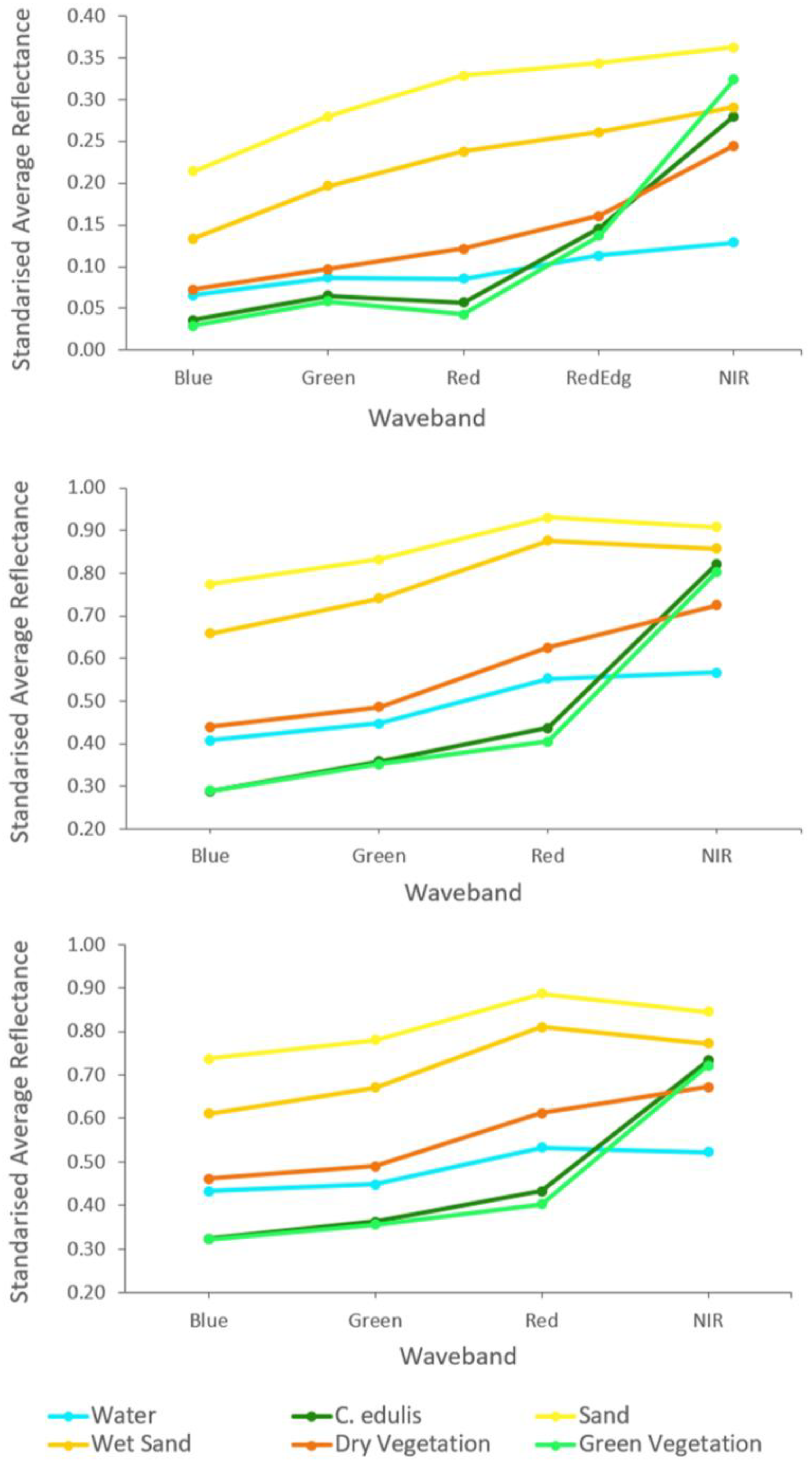
 Table 5 and Figure 6 show that, even though there was sufficient differentiation between the spectral signature of green vegetation and of C. edulis to provide a satisfactory classification accuracy result, a considerable overlapping of these signatures must be acknowledged. This overlapping results in uncertainties and the misclassification of C. edulis and green vegetation covers.
Misclassifications may further be accentuated by the lack of the RedEdge band in the plane-based aerial images, i.e., the 5 and 10 cm GSD images. Analysing the pairwise comparisons (Table 6, Table 7 and Table 8), it is possible to see that most cover changes occurred between C. edulis and green vegetation, which may point to an inaccuracy related to the lower spectral resolutions from the 5 and 10 cm GSD. The extra RedEdge band of the UAV camera seems to provide some additional information that enhances the classification accuracy.
A further and deeper investigation may allow for the identification of the most significant factors influencing cover discrepancies between resolutions in larger areas. An analysis of the classification confidence map for these areas may provide some helpful information.

5.2. Biomass Estimation

For the quantification of vegetation through regression models, the RDVI, ENDVI, and GCI exhibited the best performance for the 2.5, 5, and 10 cm GSD, respectively. Several previous investigations have achieved promising outcomes when employing the NDVI to assess various measurable attributes of vegetation [42,43,44,45,46], consolidating the NDVI’s status as the predominant index in vegetation research [47]. However, within the context of this study, the NDVI occupied a relatively low position as the eighth, seventh, and fifth most effective model for DW prediction for the 2.5, 5, and 10 cm GSD, respectively (Appendix ATable A4). This corroborates prior research indicating that various vegetation indices (VIs) may exhibit stronger correlations with vegetation AGB and quantitative attributes, compared to the conventional NDVI [45]. Consequently, the development of a specific methodology for evaluating the predictive accuracy of diverse VIs in relation to vegetation attributes still requires investigation. To do so, it is crucial to consider a wide spectrum of variables, including species diversity and topographical features, as well as weather and lighting conditions [45]. Additionally, opposed to commercial crops, the inherent morphological variability among natural vegetation species poses an additional challenge when seeking a universal relationship between image-derived data and quantifiable vegetation attributes. Consequently, a possible relationship between plant AGB and the VI must be investigated and modelled case by case [45].
Even though there is a significant difference in the C. edulis classified area between resolutions, the total AGB estimated presented similar values for the 2.5 and 5 cm GSD, yet a considerably different value for the 10 cm GSD images. For the above-mentioned reasons, the AGB estimates for the 2.5 cm resolution images were considered the most accurate. In comparison, the 5 cm GSD C. edulis area was 25% smaller but the AGB 3% larger, and the 10 cm GSD area was 33% smaller, with a 22% smaller AGB. These values show that the discrepancy in the results of the classified areas is somewhat compensated for by the estimated vegetation densities, obtained from the empirical model, as the AGB per square meter was higher for the aeroplane images than for the UAV images (Table 5).
To investigate alternative calculations for the AGB estimation, a comparison was undertaken between the already-presented total AGB obtained using the VI of individual classified C. edulis pixels and the total AGB derived using the mean VI in conjunction with the reference raster-estimated C. edulis area. The results (Table 5) suggest that the mean VI and the reference raster-estimated area of C. edulis can reasonably estimate the total AGB in the study area. Even though the errors were higher, since the 95% CI area was used, relative errors of up to 0.17 show that this method might still provide relevant insights. The final result can be compared with the result using the classified area, with both sharing a relevant overlap considering the errors. However, there is a fundamental difference between these estimations; while the total AGB based on the classified area has a geospatial distribution, meaning that it is possible to locate the C. edulis AGB inside the study area, the total AGB based on the estimated area has no spatiality, it only provides an overall estimate for the total AGB inside the study area.

5.3. Estimation Uncertainties

While this investigation has achieved favourable outcomes in forecasting DWgreen through VIs, uncertainties in the computation of the total aboveground biomass (AGB) have to be recognised. There are the widely acknowledged uncertainties inherent to classification and regression models. The orthorectification may have uncertainties, although, as the visual alignment with the sample areas (squares) displayed in the images suggested, the orthorectification did not have significant errors. And some uncertainties remain unquantifiable. For instance, the WW–DW ratio demonstrates a linear correlation, and employing a mean ratio can be a reasonable approximation. Nevertheless, this approach involves many variables that exhibit spatial and temporal variations. For instance, certain plants may thrive in more humid microenvironments compared to others, and their life stages may also differ, potentially affecting the ratio.
An even higher uncertainty is associated with the morphology of C. edulis, characterised by the presence of two distinct layers: an upper succulent green layer and a drier brown layer. This peculiarity poses a considerable challenge when estimating the AGB for a generic location using a model-based approach. Notably, no identifiable correlation was noticed between DWgreen and DWbrown, and all the regression models presented p-values greater than 0.05. Consequently, the most viable approach used a mean ratio as the best estimate. This ratio could be influenced by many factors, including plant age, growth rate, decay velocity, seasonality, and availability of water and light.
The ability to distinguish between various vegetation covers may be more or less successful, depending upon the season and the plants’ state, with spectral signatures likely varying between seasons and across regions. In the current investigation, data collection occurred during the spring season, specifically prior to flowering. This choice was made based on the belief that flowers could potentially influence the classification outcomes and biomass estimation via vegetation indices. However, a recent study [48], which involved the classification of C. edulis during the flowering season, revealed that flowers do not pose a significant impact on image classification results.
The estimation of C. edulis’ AGB plays an important role in the management of invasive species, where the biomass estimates offer critical insights for planning and executing removal campaigns. Nonetheless, the approach adopted in this study holds the potential for broader applications, extending beyond C. edulis and can be reproduced with various low-stratum plant species. Furthermore, it can be leveraged for estimating the total carbon content in ecosystems, employing established biomass–carbon correlations.
Moreover, the exploration of the feasibility of constructing a general model for predicting C. edulis DW-VI relationships could be an interesting future investigation. This endeavour requires conducting an array of new tests, mirroring the methodology employed in the current investigation, to recognise potential patterns associating the VIs with the AGB. These future investigations can also search into the utility of VIs for refining land cover classifications, thus assessing their viability in enhancing the identification of C. edulis. Relevant future research may also include an evaluation of the applicability and precision of this methodology using imagery characterised by even lower resolutions, including satellite-based images. Such assessments can serve to monitor the distribution and biomass of C. edulis on a regional scale.

6. Conclusions

In conclusion, the results obtained in this study suggest that multispectral images have a relevant potential for monitoring the invasive species C. edulis. Even though some differences were detected, all three spatial resolutions presented relevant results for monitoring, with the 2.5 and 5 cm GSD resolution being the most accurate ones. Still, the 10 cm GSD resolution can provide valuable insight on the area and AGB of C. edulis, especially when considering the multipurpose samples campaign, which might have larger pixels for monitoring more extensive areas. Regarding the spectral resolution, no significant difference was attributed to the RedEdge band on the 2.5 GSD imagery, with the four-band imagery presenting a satisfactory result. Finally, it is interesting to address that the applied methodology has the potential to be applied to a wide variety of coastal (and other) environment monitoring.

Author Contributions

Conceptualisation, M.d.F.M., J.A.G. and A.M.F.B.; methodology, M.d.F.M., J.A.G. and A.M.F.B.; software, M.d.F.M., J.A.G. and A.M.F.B.; validation, M.d.F.M. and A.M.F.B.; formal analysis, M.d.F.M. and A.M.F.B.; investigation, M.d.F.M. and A.M.F.B.; resources, J.A.G. and A.M.F.B.; data curation, M.d.F.M.; writing—original draft preparation, M.d.F.M., J.A.G. and A.M.F.B.; writing—review and editing, M.d.F.M., J.A.G. and A.M.F.B.; visualisation, M.d.F.M. and A.M.F.B.; supervision, J.A.G. and A.M.F.B.; project administration, J.A.G. and A.M.F.B.; funding acquisition, J.A.G. and A.M.F.B. All authors have read and agreed to the published version of the manuscript.

Funding

This research was partially funded by the Ocean3R (NORTE-01-0145-FEDER-000064) and ATLANTIDA (NORTE-01-0145-FEDER-000040) projects, supported by the Norte Portugal Regional Operational Program (NORTE 2020) under the PORTUGAL 2020 Partnership Agreement, and supported by national funds through the FCT—Foundation for Science and Technology within the scope of UIDB/04423/2020 and UIDP/04423/2020.

Data Availability Statement

The datasets here produced and analysed will be made available (upon request) through the institution’s geographic data server (https://gis.ciimar.up.pt).

Conflicts of Interest

The authors declare no conflicts of interest. The funders had no role in the design of the study; in the collection, analyses, or interpretation of data; in the writing of the manuscript; or in the decision to publish the results.

Appendix A

The classification accuracy results for each resolution are detailed from Table A1, Table A2 and Table A3.
Table A1. Area-based classification error matrix for the 2.5 cm GSD classification.
2.5 cm GSDReference
WaterC. edulisDry SandWet SandDry VegetationGreen Vegetation% of AreaArea
ClassifiedWater0.2620.0000.0000.0020.0000.00026.5%5980
C. edulis0.0000.1200.0000.0000.0020.03015.2%3441
Dry sand0.0000.0000.0910.0000.0100.00210.3%2329
Wet sand0.0020.0000.0020.1080.0000.00011.2%2533
Dry vegetation0.0010.0050.0160.0050.1340.01918.1%4100
Green vegetation0.0000.0060.0000.0000.0020.17918.7%4223
% of Area26.6%13.2%11.0%11.5%14.7%23.0%100.000
Area (m2)601129822478260633315198 22,605
SE area6617612890177201
95% CI area129345252177347393
PA98.7%91.0%83.3%93.5%91.2%77.7%
UA99.2%78.9%88.7%96.2%74.1%95.7%
Overall accuracy89.5%
Kappa hat0.871
Table A2. Area-based classification error matrix for the 5 cm GSD classification.
5 cm GSD Reference
WaterC. edulisDry SandWet SandDry VegetationGreen Vegetation% of AreaArea (m2)
ClassifiedWater0.2470.0000.0000.0060.0000.00025.2%5705
C. edulis0.0000.1010.0020.0000.0020.03013.6%3070
Dry sand0.0000.0000.0830.0010.0100.0019.5%2140
Wet sand0.0010.0000.0050.1070.0030.00111.6%2628
Dry vegetation0.0070.0040.0300.0120.1390.01420.6%4651
Green vegetation0.0000.0110.0020.0000.0060.17719.5%4416
% of Area25.5%11.6%12.1%12.6%16.1%22.2%100.0%
Area (m2)576126162727284536385023 22,610
SE area104160160133200190
95% CI area203314313261392372
PA96.7%87.5%68.4%84.9%86.5%79.6%
UA97.7%74.6%87.2%91.9%67.7%90.6%
Overall accuracy85.3%
Kappa hat 0.820
Table A3. Area-based classification error matrix for the 10 cm GSD classification.
10 cm GSDReference
WaterC. edulisDry SandWet SandDry VegetationGreen Vegetation% of AreaArea
ClassifiedWater0.2470.0040.0000.0000.0000.00625.7%5804
C. edulis0.0000.0850.0000.0000.0030.01410.2%2305
Dry sand0.0000.0000.0900.0000.0030.0009.3%2098
Wet sand0.0000.0000.0030.0990.0000.00010.1%2289
Dry vegetation0.0000.0060.0230.0280.1360.00620.0%4511
Green vegetation0.0000.0130.0000.0000.0050.23024.8%5604
% of Area24.7%10.8%11.5%12.7%14.8%25.6%100.0%
Area557824312603286533395795 22,610
SE area100160123127186176
95% CI area196313241248364345
PA100.0%79.0%77.8%77.9%92.3%89.8%
UA96.1%83.3%96.5%97.6%68.3%92.8%
Overall accuracy88.6%
Kappa hat0.859
The regression models relating C. edulis DW to the best-performing VI for each GSD resolution, and their respective residuals plotted are shown in Figure A1, Figure A2 and Figure A3.
Figure A1. Regression model relating C. edulis DW of sample areas to the best-performing VI for the 2.5 cm GSD: survey-sample points and regression line with equation (a), and residuals plot (b).
Remotesensing 16 00652 g0a1
Figure A2. Regression model relating C. edulis DW of sample areas to the best-performing VI for the 5 cm GSD: survey-sample points and regression line with equation (a), and residuals plot (b).
Remotesensing 16 00652 g0a2
Figure A3. Regression model relating C. edulis DW of sample areas to the best-performing VI for the 10 cm GSD: survey-sample points and regression line with equation (a), and residuals plot (b).
Remotesensing 16 00652 g0a3
Table A4. Vegetation indices empirical regression results, ordered by R2. Best-performing indices for each GSD resolution are marked in green.
Resolution RankGSDVegetation IndexModel Equationp-ValueRMSENRMSECoef. aCoef. b
12.5 cmRDVIy = abx0.868<0.0001227.1780.094151.94581.109
22.5 cmDVIy = abx0.846<0.0001234.4180.096204.547380.533
32.5 cmGDVIy = axb0.841<0.0001234.8510.09715,205.4711.984
42.5 cmRVIy = axb0.828<0.0001271.8560.112264.764−0.733
52.5 cmGCIy = axb0.808<0.0001292.9220.121355.1450.613
62.5 cmENDVIy = abx0.807<0.0001306.3800.126530.9935.144
72.5 cmGNDVIy = abx0.795<0.0001301.8120.12431.9445.201
82.5 cmNDVIy = abx0.793<0.0001316.7960.130130.45319.155
15 cmENDVIy = abx0.767<0.0001300.6750.1242596.48313.48
92.5 cmPRIy = abx0.766<0.0001334.3710.138199.192111.099
25 cmGCIy = abx0.763<0.0001286.2780.118439.552.762
35 cmRVIy = axb0.757<0.0001305.3700.126357.892−1.826
45 cmGNDVIy = abx0.755<0.0001312.0750.128128.654326.561
55 cmNDVIy = abx0.753<0.0001311.9930.128341.06853.151
65 cmGDVIy = abx0.752<0.0001299.7840.123118.118174.225
75 cmRDVIy = abx0.750<0.0001310.3100.128327.3841.328
85 cmDVIy = abx0.740<0.0001314.4350.129316.12431.858
110 cmGCIy = abx0.644<0.0001364.5520.150506.4363.068
210 cmDVIy = abx0.641<0.0001363.2820.150420.96733.223
310 cmRDVIy = abx0.639<0.0001369.5990.152429.32738.289
410 cmRVIy = axb0.637<0.0001375.0400.154448.837−1.787
510 cmENDVIy = abx0.634<0.0001374.6500.1543111.19911.267
610 cmNDVIy = abx0.634<0.0001378.1910.156439.31243.577
710 cmGDVIy = abx0.630<0.0001358.4060.148213.865123.69
810 cmGNDVIy = abx0.620<0.0001383.2280.158223.962155.699
95 cmPRIy = abx0.601<0.0001411.6310.169257.4516,134,559.7
910 cmPRIy = abx0.4490.0001457.0380.188381.254,745,123,015.5

References

  1. Tu, W.; Zhang, Y.; Li, Q.; Mai, K.; Cao, J. Scale Effect on Fusing Remote Sensing and Human Sensing to Portray Urban Functions. IEEE Geosci. Remote Sens. Lett. 2021, 18, 38–42. [Google Scholar] [CrossRef]
  2. Stückemann, K.-J.; Waske, B. Mapping Lower Saxony’s Salt Marshes Using Temporal Metrics of Multi-Sensor Satellite Data. Int. J. Appl. Earth Obs. Geoinf. 2022, 115, 103123. [Google Scholar] [CrossRef]
  3. Doughty, C.L.; Ambrose, R.F.; Okin, G.S.; Cavanaugh, K.C. Characterizing Spatial Variability in Coastal Wetland Biomass across Multiple Scales Using UAV and Satellite Imagery. Remote Sens. Ecol. Conserv. 2021, 7, 411–429. [Google Scholar] [CrossRef]
  4. Zhou, Z.; Yang, Y.; Chen, B. Estimating Spartina Alterniflora Fractional Vegetation Cover and Aboveground Biomass in a Coastal Wetland Using SPOT6 Satellite and UAV Data. Aquat. Bot. 2018, 144, 38–45. [Google Scholar] [CrossRef]
  5. Guo, M.; Li, J.; Sheng, C.; Xu, J.; Wu, L. A Review of Wetland Remote Sensing. Sensors 2017, 17, 777. [Google Scholar] [CrossRef]
  6. Li, R.; Gao, X.; Shi, F.; Zhang, H. Scale Effect of Land Cover Classification from Multi-Resolution Satellite Remote Sensing Data. Sensors 2023, 23, 6136. [Google Scholar] [CrossRef]
  7. Gann, D.; Richards, J. Scaling of Classification Systems—Effects of Class Precision on Detection Accuracy from Medium Resolution Multispectral Data. Landsc. Ecol. 2023, 38, 659–687. [Google Scholar] [CrossRef]
  8. Chen, J.; Chen, Z.; Huang, R.; You, H.; Han, X.; Yue, T.; Zhou, G. The Effects of Spatial Resolution and Resampling on the Classification Accuracy of Wetland Vegetation Species and Ground Objects: A Study Based on High Spatial Resolution UAV Images. Drones 2023, 7, 61. [Google Scholar] [CrossRef]
  9. Bhatt, P.; Maclean, A.L. Comparison of High-Resolution NAIP and Unmanned Aerial Vehicle (UAV) Imagery for Natural Vegetation Communities Classification Using Machine Learning Approaches. GIScience Remote Sens. 2023, 60, 2177448. [Google Scholar] [CrossRef]
  10. Mishra, V.N.; Rai, P.K.; Kumar, P.; Prasad, R. Evaluation of Land Use/Land Cover Classification Accuracy Using Multi-Resolution Remote Sensing Images. Forum Geogr. 2016, XV, 45–53. [Google Scholar] [CrossRef]
  11. Chen, D.; Stow, D.A.; Gong, P. Examining the Effect of Spatial Resolution and Texture Window Size on Classification Accuracy: An Urban Environment Case. Int. J. Remote Sens. 2004, 25, 2177–2192. [Google Scholar] [CrossRef]
  12. Gao, Y.; Mas, J.F. A Comparison of the Performance of Pixel-Based and Object-Based Classifications over Images with Various Spatial Resolutions. Online J. Earth Sci. 2008, 2, 27–35. [Google Scholar]
  13. Goward, S.N.; Davis, P.E.; Fleming, D.; Miller, L.; Townshend, J.R. Empirical Comparison of Landsat 7 and IKONOS Multispectral Measurements for Selected Earth Observation System (EOS) Validation Sites. Remote Sens. Environ. 2003, 88, 80–99. [Google Scholar] [CrossRef]
  14. Hsieh, P.F.; Lee, L.C.; Chen, N.Y. Effect of Spatial Resolution on Classification Errors of Pure and Mixed Pixels in Remote Sensing. IEEE Trans. Geosci. Remote Sens. 2001, 39, 2657–2663. [Google Scholar] [CrossRef]
  15. Gonçalves, C.; Santana, P.; Brandão, T.; Guedes, M. Automatic Detection of Acacia Longifolia Invasive Species Based on UAV-Acquired Aerial Imagery. Inf. Process. Agric. 2022, 9, 276–287. [Google Scholar] [CrossRef]
  16. Mallmann, C.L.; Zaninni, A.F.; Filho, W.P. Vegetation Index Based in Unmanned Aerial Vehicle (Uav) to Improve the Management of Invasive Plants in Protected Areas, Southern Brazil. In Proceedings of the 2020 IEEE Latin American GRSS & ISPRS Remote Sensing Conference (LAGIRS), Santiago, Chile, 22–26 March 2020; pp. 66–69. [Google Scholar]
  17. Huete, A.; Lyon, J.G.; Thenkabail, P.S. Hyperspectral Remote Sensing of Vegetation, 2nd ed.; CRC Press: New York, NY, USA, 2016; ISBN 978-1-4398-4538-7. [Google Scholar]
  18. Yang, S.; Hu, L.; Wu, H.; Ren, H.; Qiao, H.; Li, P.; Fan, W. Integration of Crop Growth Model and Random Forest for Winter Wheat Yield Estimation from UAV Hyperspectral Imagery. IEEE J. Sel. Top. Appl. Earth Obs. Remote Sens. 2021, 14, 6253–6269. [Google Scholar] [CrossRef]
  19. Li, B.; Xu, X.; Zhang, L.; Han, J.; Bian, C.; Li, G.; Liu, J.; Jin, L. Above-Ground Biomass Estimation and Yield Prediction in Potato by Using UAV-Based RGB and Hyperspectral Imaging. ISPRS J. Photogramm. Remote Sens. 2020, 162, 161–172. [Google Scholar] [CrossRef]
  20. Santos, L.M.; Ferraz, G.A.S.; Diotto, A.V.; Barbosa, B.D.S.; Maciel, D.T.; Andrade, M.T.; Ferraz, P.F.P.; Rossi, G. Coffee Crop Coefficient Prediction as a Function of Biophysical Variables Identified from RGB UAS Images. Agron. Res. 2020, 18, 1463–1471. [Google Scholar] [CrossRef]
  21. Wengert, M.; Wijesingha, J.; Schulze-Brüninghoff, D.; Wachendorf, M.; Astor, T. Multisite and Multitemporal Grassland Yield Estimation Using UAV-Borne Hyperspectral Data. Remote Sens. 2022, 14, 2068. [Google Scholar] [CrossRef]
  22. Wijesingha, J.; Astor, T.; Schulze-Brüninghoff, D.; Wachendorf, M. Mapping Invasive Lupinus Polyphyllus Lindl. in Semi-Natural Grasslands Using Object-Based Image Analysis of UAV-Borne Images. PFG J. Photogramm. Remote. Sens. Geoinformation Sci. 2020, 88, 391–406. [Google Scholar] [CrossRef]
  23. Brunel, S.; Brundu, G.; Fried, G. Eradication and Control of Invasive Alien Plants in the M Editerranean B Asin: Towards Better Coordination to Enhance Existing Initiatives. EPPO Bull. 2013, 43, 290–308. [Google Scholar] [CrossRef]
  24. Gomes, P.T.; Botelho, A.A.; Soares de Carvalho, G. Sistemas Dunares do Litoral de Esposende; Universidade do Minho: Braga, Portugal, 2002; ISBN 978-972-9027-16-1. [Google Scholar]
  25. Carvalho, G.S.; Granja, H.M.; Gomes, P.; Loureiro, E.; Henriques, R.; Carrilho, I.; Costa, A.L.; Ribeiro, P. New Data and New Ideas Concerning Recent Geomorphological Changes in the NW Coastal Zone of Portugal. In Proceedings of the 6th International Symposium Proceedings—The Changing Coast, Porto, Portugal, 22–26 September 2002. [Google Scholar]
  26. Conser, C.; Connor, E.F. Assessing the Residual Effects of Carpobrotus Edulis Invasion, Implications for Restoration. Biol. Invasions 2009, 11, 349–358. [Google Scholar] [CrossRef]
  27. Meyer, M.D.F.; Gonçalves, J.A.; Cunha, J.F.R.; Ramos, S.C.D.C.E.S.; Bio, A.M.F. Application of a Multispectral UAS to Assess the Cover and Biomass of the Invasive Dune Species Carpobrotus edulis. Remote Sens. 2023, 15, 2411. [Google Scholar] [CrossRef]
  28. Gitelson, A.A. Remote Estimation of Canopy Chlorophyll Content in Crops. Geophys. Res. Lett. 2005, 32, L08403. [Google Scholar] [CrossRef]
  29. Richardson, A.D.; Duigan, S.P.; Berlyn, G.P. An Evaluation of Noninvasive Methods to Estimate Foliar Chlorophyll Content. N. Phytol. 2002, 153, 185–194. [Google Scholar] [CrossRef]
  30. Tucker, C.J.; Elgin, J.H.; McMurtrey, J.E.; Fan, C.J. Monitoring Corn and Soybean Crop Development with Hand-Held Radiometer Spectral Data. Remote Sens. Environ. 1979, 8, 237–248. [Google Scholar] [CrossRef]
  31. Rasmussen, J.; Ntakos, G.; Nielsen, J.; Svensgaard, J.; Poulsen, R.N.; Christensen, S. Are Vegetation Indices Derived from Consumer-Grade Cameras Mounted on UAVs Sufficiently Reliable for Assessing Experimental Plots? Eur. J. Agron. 2016, 74, 75–92. [Google Scholar] [CrossRef]
  32. Gitelson, A.A.; Kaufman, Y.J.; Merzlyak, M.N. Use of a Green Channel in Remote Sensing of Global Vegetation from EOS-MODIS. Remote Sens. Environ. 1996, 58, 289–298. [Google Scholar] [CrossRef]
  33. Rouse, J.W.; Haas, R.H.; Deering, D.W.; Schell, J.A.; Harlan, J.C. Monitoring the Vernal Advancement and Retrogradation (Green Wave Effect) of Natural Vegetation; Great Plains Corridor; NASA: Washington, DC, USA, 1973. [Google Scholar]
  34. Gamon, J.A.; Peñuelas, J.; Field, C.B. A Narrow-Waveband Spectral Index That Tracks Diurnal Changes in Photosynthetic Efficiency. Remote Sens. Environ. 1992, 41, 35–44. [Google Scholar] [CrossRef]
  35. Roujean, J.-L.; Breon, F.-M. Estimating PAR Absorbed by Vegetation from Bidirectional Reflectance Measurements. Remote Sens. Environ. 1995, 51, 375–384. [Google Scholar] [CrossRef]
  36. Pearson, R.L.; Miller, L.D. Remote Mapping of Standing Crop Biomass for Estimation of the Productivity of the Shortgrass Prairie. Remote Sens. Environ. 1972, VIII, 1355. [Google Scholar]
  37. Olofsson, P.; Foody, G.M.; Herold, M.; Stehman, S.V.; Woodcock, C.E.; Wulder, M.A. Good Practices for Estimating Area and Assessing Accuracy of Land Change. Remote Sens. Environ. 2014, 148, 42–57. [Google Scholar] [CrossRef]
  38. Karasiak, N. Dzetsaka Qgis Classification Plugin. 2016. Available online: https://github.com/nkarasiak/dzetsaka (accessed on 27 August 2022).
  39. Congedo, L. Semi-Automatic Classification Plugin: A Python Tool for the Download and Processing of Remote Sensing Images in QGIS. J. Open Source Softw. 2021, 6, 3172. [Google Scholar] [CrossRef]
  40. Papp, L.; van Leeuwen, B.; Szilassi, P.; Tobak, Z.; Szatmári, J.; Árvai, M.; Mészáros, J.; Pásztor, L. Monitoring Invasive Plant Species Using Hyperspectral Remote Sensing Data. Land 2021, 10, 29. [Google Scholar] [CrossRef]
  41. Michez, A.; Piégay, H.; Jonathan, L.; Claessens, H.; Lejeune, P. Mapping of Riparian Invasive Species with Supervised Classification of Unmanned Aerial System (UAS) Imagery. Int. J. Appl. Earth Obs. Geoinf. 2016, 44, 88–94. [Google Scholar] [CrossRef]
  42. Guan, S.; Fukami, K.; Matsunaka, H.; Okami, M.; Tanaka, R.; Nakano, H.; Sakai, T.; Nakano, K.; Ohdan, H.; Takahashi, K. Assessing Correlation of High-Resolution NDVI with Fertilizer Application Level and Yield of Rice and Wheat Crops Using Small UAVs. Remote Sens. 2019, 11, 112. [Google Scholar] [CrossRef]
  43. Hassan, M.A.; Yang, M.; Rasheed, A.; Yang, G.; Reynolds, M.; Xia, X.; Xiao, Y.; He, Z. A Rapid Monitoring of NDVI across the Wheat Growth Cycle for Grain Yield Prediction Using a Multi-Spectral UAV Platform. Plant Sci. 2019, 282, 95–103. [Google Scholar] [CrossRef]
  44. Pandey, P.C.; Anand, A.; Srivastava, P.K. Spatial Distribution of Mangrove Forest Species and Biomass Assessment Using Field Inventory and Earth Observation Hyperspectral Data. Biodivers. Conserv. 2019, 28, 2143–2162. [Google Scholar] [CrossRef]
  45. Huang, S.; Tang, L.; Hupy, J.P.; Wang, Y.; Shao, G. A Commentary Review on the Use of Normalized Difference Vegetation Index (NDVI) in the Era of Popular Remote Sensing. J. For. Res. 2021, 32, 2719. [Google Scholar] [CrossRef]
  46. Tenreiro, T.R.; García-Vila, M.; Gómez, J.A.; Jiménez-Berni, J.A.; Fereres, E. Using NDVI for the Assessment of Canopy Cover in Agricultural Crops within Modelling Research. Comput. Electron. Agric. 2021, 182, 106038. [Google Scholar] [CrossRef]
  47. Xu, Y.; Yang, Y.; Chen, X.; Liu, Y. Bibliometric Analysis of Global NDVI Research Trends from 1985 to 2021. Remote Sens. 2022, 14, 3967. [Google Scholar] [CrossRef]
  48. Innangi, M.; Marzialetti, F.; Di Febbraro, M.; Acosta, A.T.R.; De Simone, W.; Frate, L.; Finizio, M.; Villalobos Perna, P.; Carranza, M.L. Coastal Dune Invaders: Integrative Mapping of Carpobrotus Sp. Pl. (Aizoaceae) Using UAVs. Remote Sens. 2023, 15, 503. [Google Scholar] [CrossRef]
Figure 1. Location of study area (red) in Iberian Peninsula (a); study area (b).
Remotesensing 16 00652 g001
Figure 2. Placement of a quadrat on a C. edulis patch, with other vegetation covers visible to the left (various herbaceous species) and in the back (acacia) (a); delimitation of the central 30 × 30 cm2 area within a quadrat for AGB removal (b); brown layer of C. edulis after removal of the top green layer (c).
Remotesensing 16 00652 g002
Figure 3. Orthomosaic image with 10 cm GSD and ROI points marked.
Remotesensing 16 00652 g003
Figure 4. ROI for C. edulis when located over a homogeneous area (a) and located over a non-homogeneous area (b).
Remotesensing 16 00652 g004
Figure 5. Representative area of the land cover classification for each of the resolutions.
Remotesensing 16 00652 g005
Figure 6. Mean spectral signatures of ROI divided by class and GSD orthomosaic.
Remotesensing 16 00652 g006
Figure 7. Comparison of F1 score for the C. edulis class for different filters (4: 4-pixel filter; 8: 8-pixel filter), thresholds, and resolutions. Highest F1 score marked in red.
Remotesensing 16 00652 g007
Figure 8. Cover class distribution for the classification results obtained with each spatial resolution; labels in the graphic indicate area in square meters.
Remotesensing 16 00652 g008
Figure 9. Orthomosaic cover changes comparison between resolutions, for the areas classified as C. edulis, comparing change from: 2.5 cm to 5 cm GSD (a); 5 cm to 10 cm GSD (b); 2.5 cm to 10 cm GSD (c).
Remotesensing 16 00652 g009
Table 1. Vegetation indices formulas used in this work. Bands: Blu—Blue; Gre—Green; NIR—Near-Infrared.
IndexFormulaReference
Green Chlorophyll Index (GCI) N I R R e d 1 [28]
Difference Vegetation Index (DVI) N I R R e d [29]
Green Difference Vegetation Index (GDVI) N I R G r e [30]
Enhanced Normalised Difference Vegetation Index (ENDVI) N I R G r e 2 R e d N I R G r e + 2 R e d [31]
Green Normalised Difference Vegetation Index (GNDVI) N I R G r e N I R + G r e [32]
Normalised Difference Vegetation Index (NDVI) N I R R e d N I R + R e d [33]
Photochemical Reflectance Index (PRI) G r e B l u G r e + B l u [34]
Renormalised Difference Vegetation Index (RDVI) N I R R e d N I R + R e d [35]
Ratio Vegetation Index (RVI) R e d N I R [36]
Table 2. ROIs and training pixels count per resolution.
GSD (cm)Individual ROI Area (cm)Pixels per ROINumber of ROIs per ClassTotal Training Pixel Count
2.520 × 2064–813013,269
5.020 × 201612011,520
10.020 × 20446011,524
Table 3. Summary statistics of C. edulis sample wet weights (WWs) and dry weights (DWs) for the plants’ green and brown parts (SD: standard deviation).
GREENBROWN
WW (kg/m2)DW (kg/m2)WW (kg/m2)DW (kg/m2)
Highest27.122.863.652.64
Lowest2.094.6600
Mean9.681.271.010.62
Median8.161.070.510.29
SD6.430.711.130.73
Table 4. Best DWgreen–VI regression model for each resolution with respective R2, RMSE, NRMSE, model, and respective coefficients a and b.
GSD (cm)IndexR2RMSE
(kg/m2)
NRMSEModelCoef aCoef b
2.5RDVI0.870.230.09 y = a b x 151.9481.11
5ENDVI0.770.300.12 y = a b x 2596.4813.48
10GCI0.640.360.15 y = a b x 506.443.07
Table 5. Classification results, AGB values, and total AGB estimates considering the classified and estimated areas; the estimated area is calculated based on accuracy and validation samples and, considering its error, a good predictor for the real area.
Image Resolution
2.5 cm5 cm10 cm
ClassificationFilter threshold10244096256
C. edulis classified area (m2)344130702305
F1 score C. edulis84.580.581.1
Overall Accuracy89.5%85.3%88.6%
Kappa0.8710.8080.859
C. edulis estimated area (m2)298226162431
Standard error of estimated area (m2)176160160
95% confidence interval estimated area (m2)345314313
AGB values (WW)
Based on VI
empirical models
RMSE (kg/m2)0.230.300.36
Highest value (kg/m2)29.1329.1824.50
Lowest value (kg/m2)1.231.803.58
Mean (kg/m2)8.239.509.60
Median (kg/m2)7.679.449.41
Standard deviation (kg/m2)3.663.162.88
Total AGB classified areaTotal AGB (kg)28,32729,17022,135
Regression model error (RMSE × classified area) (kg)782923840
Classified area error (kg)144915201537
Total AGB error (kg)223124432377
Relative error0.080.080.11
Total AGB Estimated areaTotal AGB (kg)24,54824,85723,345
Total AGB error (kg)223124432377
95% CI AGB error (kg)351837703892
Fractional error (Total AGB error)0.090.100.10
Fractional error (95% CI AGB error)0.140.150.17
Table 6. Comparison of the cover class areas resulting from the 2.5 and 5 cm GSD classifications.
5 cm GSD
WaterC. edulisDry SandWet SandDry VegetationGreen VegetationTotal 2.5 cm GSD Area (m2)
2.5 cm GSDWater555532103298165979
C. edulis02548963005743440
Dry sand8015168526504162328
Wet sand3798823494502532
Dry vegetation2314332713132741974098
Green vegetation434923822536094221
Total 5 cm GSD area (m2)57013069213826274649441622,602
Table 7. Comparison of the cover class areas resulting from the 5 and 10 cm GSD classifications.
10 cm GSD
WaterC. edulisDry SandWet SandDry VegetationGreen VegetationTotal 5 cm GSD Area (m2)
5 cm GSDWater560400148505704
C. edulis1202950849463069
Dry sand09177476263132138
Wet sand831013218732482627
Dry vegetation4179295836545654645
Green vegetation66175609640694413
Total 10 cm GSD area (m2)57982304209522874509560322,599
Table 8. Comparison of the cover class areas resulting from the 2.5 and 10 cm GSD classifications.
10 cm GSD
WaterC. edulisDry SandWet SandDry VegetationGreen VegetationTotal 2.5 cm GSD Area (m2)
2.5 cm GSDWater55640530367115979
C. edulis10207514014311943438
Dry sand8015177232414122327
Wet sand53836217225662532
Dry vegetation33872524832044684093
Green vegetation5211814312239094219
Total 10 cm GSD area (m2)57942304209422874508560222,592
Disclaimer/Publisher’s Note: The statements, opinions and data contained in all publications are solely those of the individual author(s) and contributor(s) and not of MDPI and/or the editor(s). MDPI and/or the editor(s) disclaim responsibility for any injury to people or property resulting from any ideas, methods, instructions or products referred to in the content.

