Article

Inversion of Tidal Flat Topography Based on the Optimised Inundation Frequency Method—A Case Study of Intertidal Zone in Haizhou Bay, China

1
College of Oceanic and Atmospheric Sciences, Ocean University of China, Qingdao 266100, China
2
Key Laboratory of Ocean Space Resource Management Technology, Ministry of Natural Resources, Hangzhou 310012, China
3
Marine Academy of Zhejiang Province, Hangzhou 310012, China
*
Author to whom correspondence should be addressed.
These authors contributed equally to this work.
Remote Sens. 2024, 16(4), 685; https://doi.org/10.3390/rs16040685
Submission received: 10 January 2024 / Revised: 6 February 2024 / Accepted: 11 February 2024 / Published: 15 February 2024

Abstract

:
Coastal tidal flat wetlands are valuable natural resources that provide diverse habitats and important ecological barriers. The physical environment of the intertidal zone poses many challenges to the monitoring of tidal flat topography, making it difficult to implement traditional measurement methods, and satellite remote sensing combined with tide level information makes it possible to invert coastal tidal flat topography more conveniently over large areas. Current methods based on inundation frequency fail to consider the effect of water level distribution of remote sensing images, and usually use all available remote sensing images. However, the uneven distribution of image tide levels will increase the error of the tidal flat construction. Therefore, in this study, according to the distribution characteristics of the water level in remote sensing images, we adaptively exclude the images with a concentrated water level distribution, so as to make the water level distribution more uniform, and thus reduce the topographic inversion error. The validation results of the inversion accuracy show that the root mean squared error of the tidal flat topographic inversion improved by about 5 cm compared with the previous inundation frequency method, which is suitable for reconstructing the tidal flat topography on a large scale and a long-time scale, and it can be used as a basis for coastal tidal flat protection and restoration decision making.

1. Introduction

Tidal flats, the ocean areas between the mean high tide line and the mean low tide line, are an important wetland type and provide ample land resources [1,2]. Located in the area where land and sea intersect, tidal flats are an important transition zone between terrestrial and marine ecosystems [3,4], stabilising the coastline, buffering storms and waves, and providing breeding and nursery sites, with other ecological functions [5,6]. In recent years, the tidal flat resources in China’s coastal areas have been increasingly developed, and while great achievements have been made, problems such as excessive reclamation have arisen. As a result, serious pollution and biological invasions occurred, which led to more serious degradation in tidal flat wetlands [7,8]. From 1986 to 2016, the area of tidal flats in China decreased by nearly 1.23 × 10⁵ ha [4]. The evolution of tidal flats is the main scientific basis for their protection and rational development, and obtaining the dynamic status of tidal flats is necessary for the management, protection, and restoration of tidal flat ecosystems [9,10].
Global tidal flat topography is the basis for coastal-related studies on a global scale [11], but it is still difficult to obtain the data set at present. Obtaining information on the extent and topography of the intertidal zone is a challenging and expensive endeavour, as the region is covered by periodic seawater inundations [12,13]. Traditional methods used to map coastal bathymetry include airborne Light Detection and Ranging (LiDAR) instruments and ship-based single/multi-beam echo sounders, among others [14,15]. They are highly restricted due to their limited spatial coverage, high economic cost, and low efficiency [16]. Moreover, it is difficult for traditional measurement techniques to quickly and accurately monitor the dynamics of coastal tidal flats in a long time series [17], whereas remote sensing technology has the advantages of wide-range monitoring, short cycles, sustainability, a large amount of information, cost-effectiveness, etc. The application of remote sensing technology to the study of tidal flat evolution can achieve a comprehensive, rapid, dynamic, and accurate analysis of tidal flats [18]. It is more suitable for large-scale constructions of intertidal terrain, which is more socially and economically beneficial than traditional methods.
A variety of remote sensing-based mapping methods for tidal flats have been proposed. Existing remote sensing-based methods for mapping tidal flat topography can be divided into three types: the mean slope method, the waterline method, and the inundation frequency method [15,19,20]. The mean slope method extracts two water edges at different planar locations, assigns a tide level value to the image at the imaging moment, calculates the slope of the tidal flats based on the equirectangular triangle theory, and constructs a DEM of the tidal flats by combining the mean high tide level and the mean low tide level [19]. It is a convenient method with fewer remote sensing images to process and is suitable for areas with a flat topography and a single slope. However, this method is not suitable for tidal flats with large changes in profile morphology, and it is difficult to achieve topographic constructions in areas with many tidal channels. The waterline method solves the above limitations by obtaining multiple remote sensing images of the land and water demarcation line, and then approximating it as a contour line, assigning elevation values to it using the tide level information, and then constructing the tidal flat topography via spatial interpolation [20,21,22]. This method is relatively simple, and the data it uses are easy to obtain and highly stable, and have been widely used. However, the waterline method relies too much on tidal height information, which is used to calibrate the waterline and is often inaccurate [16]. In addition, the waterlines generated using the above method are usually discontinuous and fragmented, requiring extensive manual modifications [23].
To avoid relying on tidal heights during image acquisition, scholars have further proposed the inundation frequency method. The inundation frequency method classifies waters by applying the Modified Normalised Difference Water Index (hereinafter referred to as the MNDWI) to each remotely sensed image and normalises the probability of water exposure to create a map of the probability of inundation, and then converts the probability to an actual elevation [15]. Within the tidal flats, pixels with the same inundation frequency correspond to the same elevation, which allows the construction of time-averaged contours for the entire inversion period. In contrast, in conventional waterline-based methods, each waterline is derived from a single satellite image, which inevitably introduces elevation errors due to spatial variations and fluctuations in local water levels caused by various hydrodynamic processes [11]. The use of the intertidal inundation frequency not only provides a pixel-level elevation estimation [16], but also avoids the labour-intensive waterline extraction process and the errors caused by waterline delineation bias [19]. Previous studies have often used all the images when using the inundation frequency method, failing to take into account the effect of the image tidal height distribution, and the following is usually assumed: the higher the number of remote sensing images used, the higher the accuracy of the inversion of the tidal flat topography [16,24]. However, the uneven distribution of tide heights corresponding to remotely sensed images can cause their inundation frequency to be large or small, thus increasing the error of the beach topography inversion. To address this limitation, it can be considered to make the distribution of tide levels more uniform by eliminating images with similar tide levels, to reduce the error caused by the concentration of the distribution of tide levels in the images.
Each of these three methods has its own advantages and disadvantages, and this study draws on some of these ideas, intending to obtain tidal flat topographies and their dynamics more easily and accurately. We propose a simple method to enhance the accuracy of terrain construction. In this study, we have chosen to use an inundation frequency-based method, which addresses the requirements of the mean slope method on the morphology of the tidal flat profile, while effectively reducing the dependence of the waterline method on tidal heights. In order to optimise the limitations of this method, this study combines the information on the distribution of tidal heights at the time of the remote sensing image acquisition and excludes some of the remote sensing images with similar tidal heights, so as to make the distribution of water levels in the images more homogeneous and then construct the topography of the coastal area. The impact of the method on the accuracy of the results was assessed based on the measured terrain profiles, compared and analysed in terms of the differences between the use of all available remote sensing imagery and the filtered results. The second part of the article presents an overview of the study area, the third part describes the data and the methodology of the optimisation, the fourth part describes the results, and finally, the uncertainty of the optimisation methodology and the reasons for achieving the optimisation are discussed.

2. Study Area

The study area was located at the border between Jiangsu Province and Shandong Province, an open bay on the western side of the South Yellow Sea (Figure 1). The coastline of the study area is about 170 km long and covered an area of 876.3 km2 [25]. Jiangsu Province is the province with the widest distribution of tidal flats in China, and Haizhou Bay is a typical representative of the tidal flats in northern Jiangsu Province, where a high tidal range of up to 4 m makes the distribution of tidal flats in this region more extensive. There are six major estuaries in the study area, and these estuaries are the main source of sediment in Haizhou Bay. The Haizhou Bay area is mainly a sandy, silty and bedrock harbour coast, which provides a suitable habitat for birds and has become an important migratory stopover in the East Asia–Australia migration corridor [26]. Under the influence of sea farming and harbour construction activities, the shoreline morphology of Haizhou Bay has changed considerably, which has a great impact on the tidal flats and siltation of the beaches in the area. It is a natural place for studying the impact of human activities on the evolution of tidal flats and siltation of the beaches.

3. Data and Methods

3.1. Data

The Landsat series of images is the most widely used source of data for mapping coastal land cover at large scales. This satellite was launched relatively early, has a time interval of 16 days between repeated images, and has a spatial resolution of 30 m. It can acquire images with a long time period and sufficient spatial resolution and is more applicable to the mudflat area of interest for this study. In contrast, the MODIS satellite images have a spatial resolution of 250 m and have a higher error for the study. The Sentinel satellites was launched relatively late, and although the spatial resolution is better than that of Landsat, the number of images that can be acquired is too small. It can acquire images with a long time period and sufficient spatial resolution. In this study, images of Landsat 5, 7, and 8 were selected from 1986 through 2020, where every five years was taken as a time period, and a total of four time periods were selected: 1986–1990, 1996–2000, 2003–2007 (images from 2008–2010 were not selected due to the large-scale reclamation project in the southern part of Haizhou Bay that occurred after 2007), and 2016–2000. The acquisition of images and all pre-processing steps were performed on the Google Earth Engine (GEE), a remote sensing cloud computing platform developed by Google (code.earthengine.google.com, accessed on 2 August 2023). According to previous studies, a five-year interval is the minimum time required to be able to satisfactorily map the tidal flat topography of a beach [15]. In this study, we did not set all the cloud content below a certain value to screen the remote sensing images, but all the images were selected because a high cloud content does not mean that the study area has a high cloud content and to ensure that a sufficient number of remote sensing images were available. Remote sensing images should be selected to cover a wide range in elevation so that the extracted beach tidal flats area is accurate. In addition, the number should be large enough to ensure that the extracted elevation is accurate. We collected 1:20,000 topographic data points mapped in 2016 for the validation and evaluation of the accuracy of the topographic inversion of the tidal flats.

3.2. TPXO9

We used tidal heights from the TPXO9 model to determine the tidal height at the time each Landsat image was acquired. TPXO is a globalised ocean tidal model that has been developed by Oregon State University and is best suited to the Laplace Tidal Equations and altimetry data in a least squares sense (www.tpxo.net, accessed on 13 August 2023). The TPXO model consists of eight primaries (M2, S2, N2, K2. K1, O1, P1, Q1, and two long-period (Mf, Mm) and three non-linear (M4, MS4, MN4) harmonic constituents of the complex amplitude [27]. TPXO9-atlas is the latest 1/30-degree resolution global solution for all coastal regions, including the Arctic and Antarctic. The number of remote sensing images obtained was acquired with the temporal distribution shown in Figure 2 to determine whether the Landsat images covered different tidal heights. In the figure, the green and blue lines represent the mean high tide and mean low tide, and we can observe that the remotely sensed images are basically between the mean high tide level and the mean low tide level, and most of the images reach the mean high tide level, while the number of images that reach the mean low tide level is less. Due to the periodicity of the tidal process, the observed tidal heights were not evenly distributed over the intertidal zone. The numbers of usable remote sensing images obtained for each period were 33, 44, 34, and 42, respectively (Figure 2a).

3.3. Methods of Land and Sea Segmentation

The MNDWI has been widely used for intertidal mapping applications [28], and has advantages over the Normalized Difference Water Index (NDWI) in urban areas, where the short-wave infrared radiation (SWIR) band of the MNDWI can handle highly turbid water [29].
M N D W I = G r e e n S W I R G r e e n + S W I R
For Landsat 5, 7 Green and SWIR bands are Band 2 and Band 5, respectively, while for Landsat 8, the Green and SWIR bands are Band 2 and Band 6, respectively. The range of the values of the MNDWI was [−1, 1], and the ocean-land segmentation line of the study area was extracted based on the grey histogram of the resulting MNDWI image.
Water bodies have different optical properties and exhibit large spectral differences in remotely sensed images [30,31,32]. The use of uniform thresholds to extract information from a wide range of water bodies has limitations [33,34]. Automated thresholding methods (and other relevant indices) may help to reduce uncertainty at this step of the process. The maximum between-class variance (OSTU method) is an excellent algorithm for adaptive threshold determination [35]. It is widely used for image segmentation due to its simplicity of computation and flexibility concerning luminance and contrast [36]. The OTSU method has been shown to have a high accuracy for waterline extraction and has also achieved satisfactory results in other studies [10,37]. It is a simple unsupervised classification that can be well scaled up to larger studies on tidal flats on coastal beaches, as large amounts of training data are not required.

3.4. Inversion of Tidal Flat Topography

Under the actions of rising and falling tides, tidal flats are periodically inundated by seawater, and the waterline therefore changes dynamically. The higher the tidal flat elevation of a beach, the less time it is inundated by seawater, and therefore, the lower its inundation probability during the tidal cycle [15]. It is based on this idea that this study calculated the inundation probability by collecting a large number of index images of water bodies in the study area, indirectly converted the inundation probability to a tidal flat elevation, and constructed a Digital Elevation Model (DEM) of the tidal flats, and the formula for calculating the inundation probability is as follows:
P ( i , j ) = 1 n S k ( i , j ) n × 100 % ,
where P(i, j) is the frequency of inundation in row i and column j, n is the number of images, and Sk(i, j) indicates whether each location is covered by seawater. Considering that the water frequency of seawater is 1, the water frequency of tidal flats should vary between 0 and 1 due to the tidal cycle.
After finding the inundation frequency of the tidal flats, this study used a linear model to invert the topography with the following equation [15]:
D E M ( i , j ) = [ ( 1 P ( i , j ) ) × ( H h H l ) + H l ] × M ( i , j )
where DEM(i, j) denotes the inverted tidal flat elevation for the (i, j)th positional pixel; P(i, j) corresponds to the frequency of inundation for each pixel within the tidal flat; Hh is the high-tide level for the current period; Hl is the lowest tidal height for the current period; and M(i, j) is the tidal flat mask matrix.
The vertical accuracy of the inundation frequency method is related to the number of remote sensing images, n, and the more remote sensing images, the higher its vertical accuracy. The vertical accuracy of the inundation frequency method is related to the number n of remote sensing images, the more remote sensing images, the higher its vertical accuracy; while its lateral tidal flat width is related to the water level at the time of remote sensing acquisition, and the wider the range of the tidal heights covered, the wider the range of its lateral extraction. As shown in Figure 2, it can be seen that these time points have an uneven distribution of tidal heights and an excessive number of remote sensing images of some similar water levels. An excessive number of similar water levels will result in a lower vertical accuracy of the tidal flats, and an overestimation or underestimation of the tidal flat elevation is possible. The ideal situation for applying the frequency method is that the image tide level is uniformly distributed, in which case the inundation frequency and topographic elevation are more consistent with the linear relationship in the inversion formula. The interval of the inundation frequency was fixed at 1/n; however, the collected tidal height distribution is not uniform, and the tidal level intervals of some images with a concentrated tidal level distribution were almost the same, in which case, the linear relationship between the inundation frequency and elevation will be weakened. Therefore, in order to ensure the use of sufficient remote sensing images, and at the same time eliminate images with very similar tide levels, this study removed the images with tide level intervals less than 1/n m from all remote sensing images in each time period, so as to make the distribution of the water levels in the images more uniform, in order to reduce the error caused by the concentration of the distribution of tide levels in the images.
When the shoreline exhibits motion, the intertidal topography changes accordingly; therefore, identifying the highly dynamic shore and masking it are critical to ensuring the accuracy of the constructed intertidal DEM [38]. The landward side of the study area mask for each time period was identified using the high-tide line, and the seaward side was harmonised to approximate the furthest boundary of the low-tide line of the tidal flats. This formula is valid only in the intertidal area, and due to the interference of the culture ponds and other disturbances, the area with a probability of being landward greater than 92% was selected as the high tide line in this study, while the area near the low tide line was selected to be approximated as the farthest boundary of the low tide line of the tidal flats due to the probability of being landward being zero, which makes it difficult to distinguish it from the other areas of the bay that have much deeper water depths.

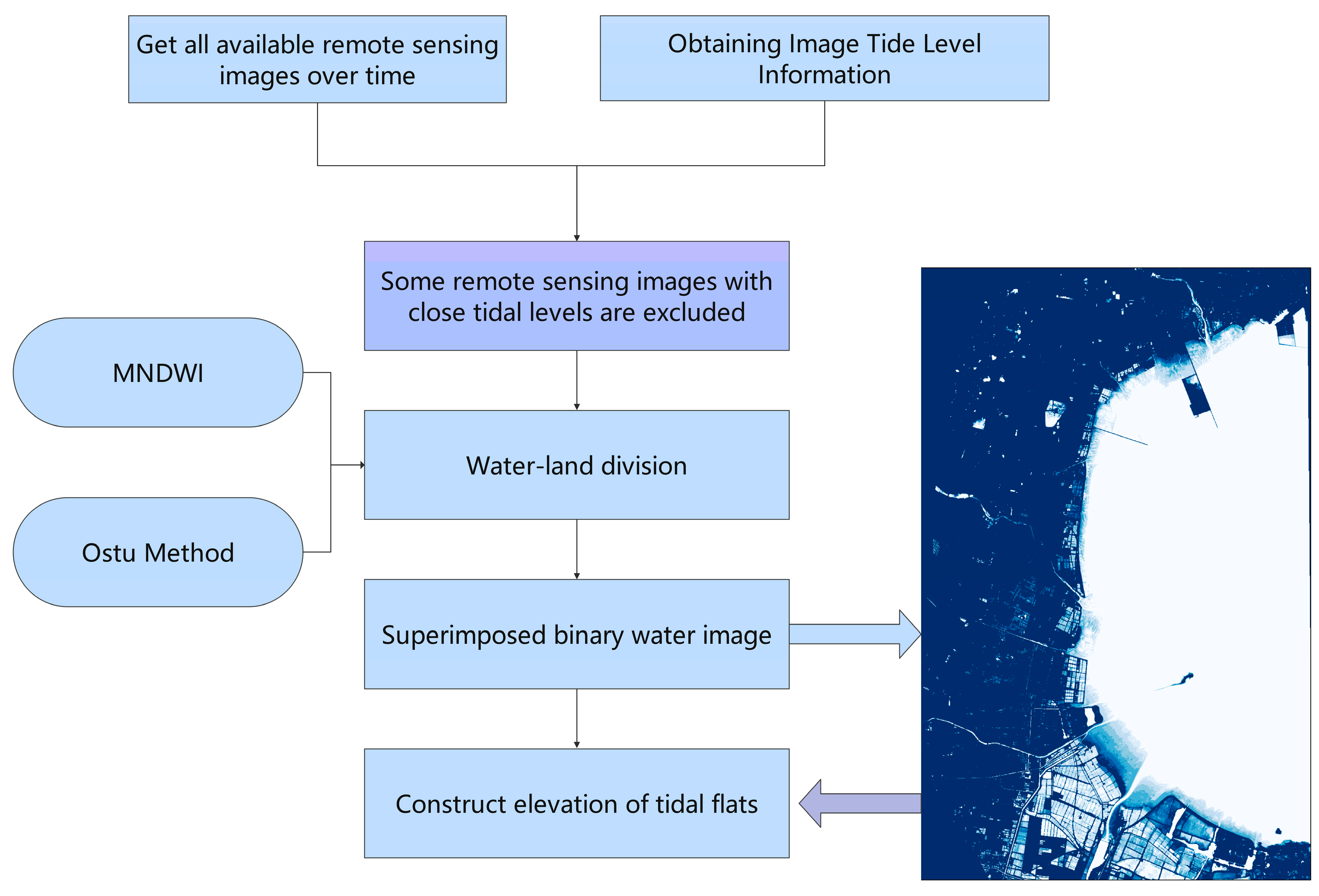
3.5. Tidal Flat Terrain Construction Process

As shown in Figure 3, to construct the tidal flats based on the inundation frequency method in this study, it is necessary to acquire a sufficient number of images, then delete the images with close tide levels, and finally construct the topographic elevation of the flats by superimposing the binarised images.

4. Results

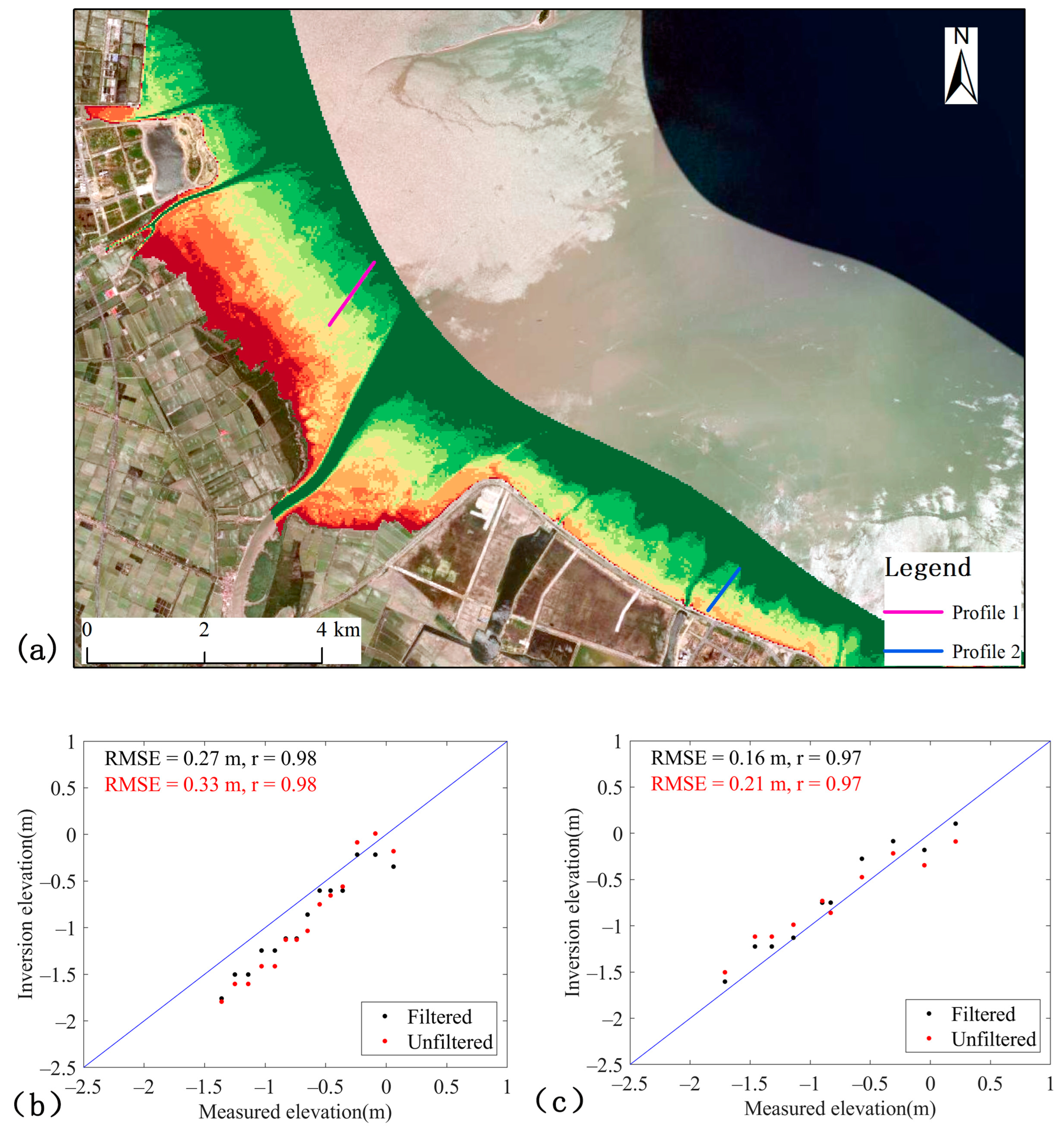
4.1. Accuracy Verification

Based on the available topographic data, the study randomly selected two profiles in the southern part of Haizhou Bay for assessment, and the profile locations are shown in Figure 4. The 2016 topographic data collected were used to assess the accuracy of the constructed topography in the southern part of Haizhou Bay during the period of 2016–2020. At the same time, we compared and analysed its results with the unscreened results of remote sensing intervals. The correlation between the inversion results of the two sections and the measured results was high, and the correlation coefficients reached more than 0.96, indicating that the difference between the inversion of the tidal flat slopes using the frequency method and the measured results was relatively small. A comparison of profile 1 and profile 2 shows that the inversion root mean squared error (RMSE) of profile 1 and profile 2 are different, and the RMSE at profile 1 is higher than that at profile 2, which may be due to the fact that profile 1 is closer to the mouth of the Linhong Estuary, and the turbidity of the water body affects the accuracy of the waterline extraction. Both profiles show that the inversion error decreases after screening remote sensing images with similar tide levels, and the inversion errors of profile 1 and profile 2 decrease by 0.04 m and 0.05 m, respectively, which suggests that the proposed method of screening remote sensing images with similar water levels can improve the inversion accuracy, and thus better invert the topography of the tidal flats.

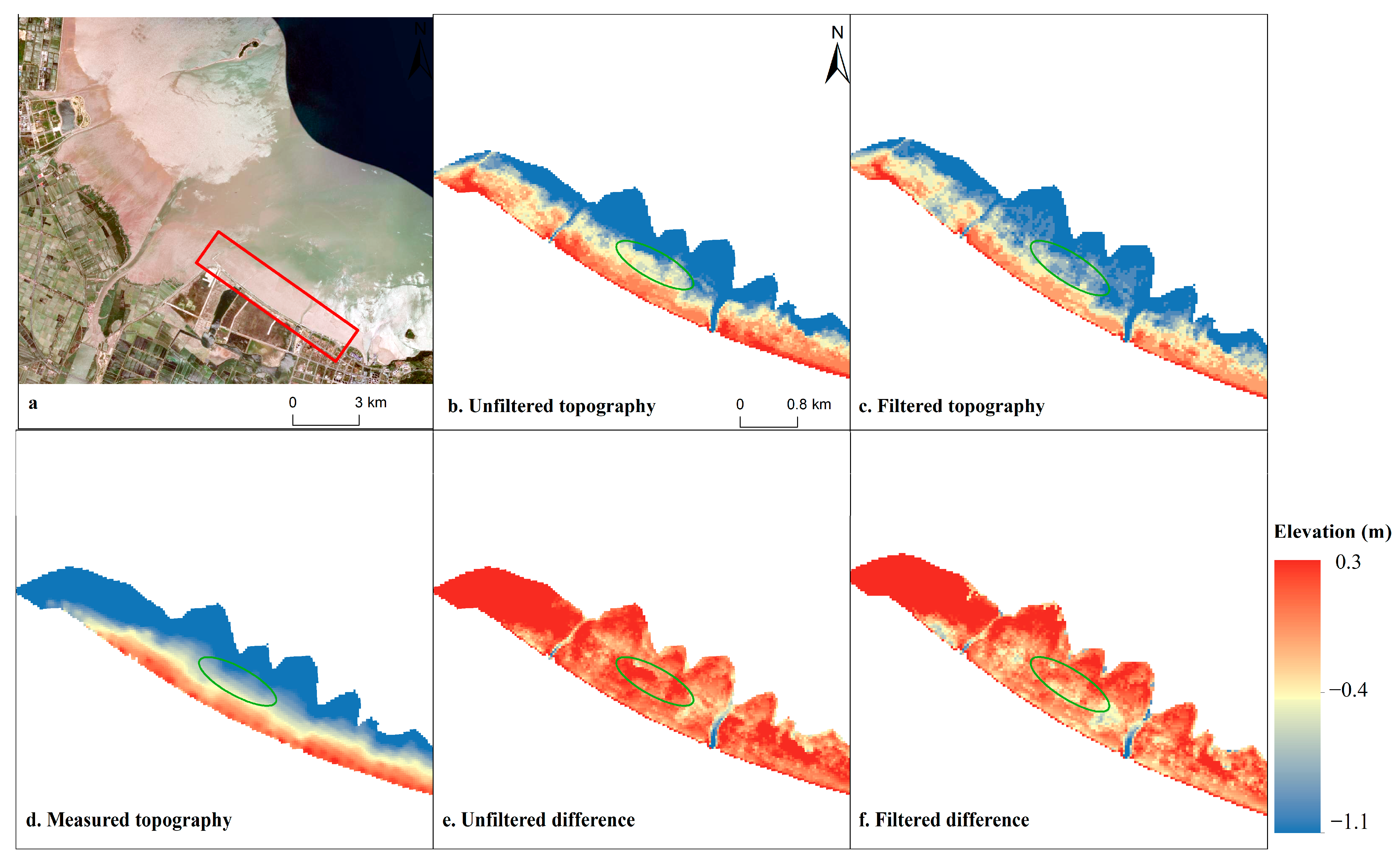
4.2. Comparison of Terrain before and after Optimisation

In this study, the red-framed area in Figure 5a was selected for spatially comparing the topographic results and analysing the similarities and differences in the DEM before and after the optimisation during 2016–2020. As shown in the figure, the topography of the tidal flats obtained using the inundation frequency method is closer to the measured topography in the overall spatial distribution, while for the left area close to and near the mouth of the Hong River, the DEM constructed using the inundation frequency method is on the high side, which may be due to the fact that this area is more affected by the river. A comparative analysis of the topography of the green box area shows that the results screened using the optimisation method are closer to the measured results, while the elevation of the unscreened topography is on the high side. In terms of specific values, the average elevation of this area is −0.88 m in the measured results, −0.62 m in the unfiltered results, and −0.70 m in the optimised filtered results. The optimised filtered DEMs have less deviation from the measured results, which further confirms the reliability of the optimised inundation frequency method.

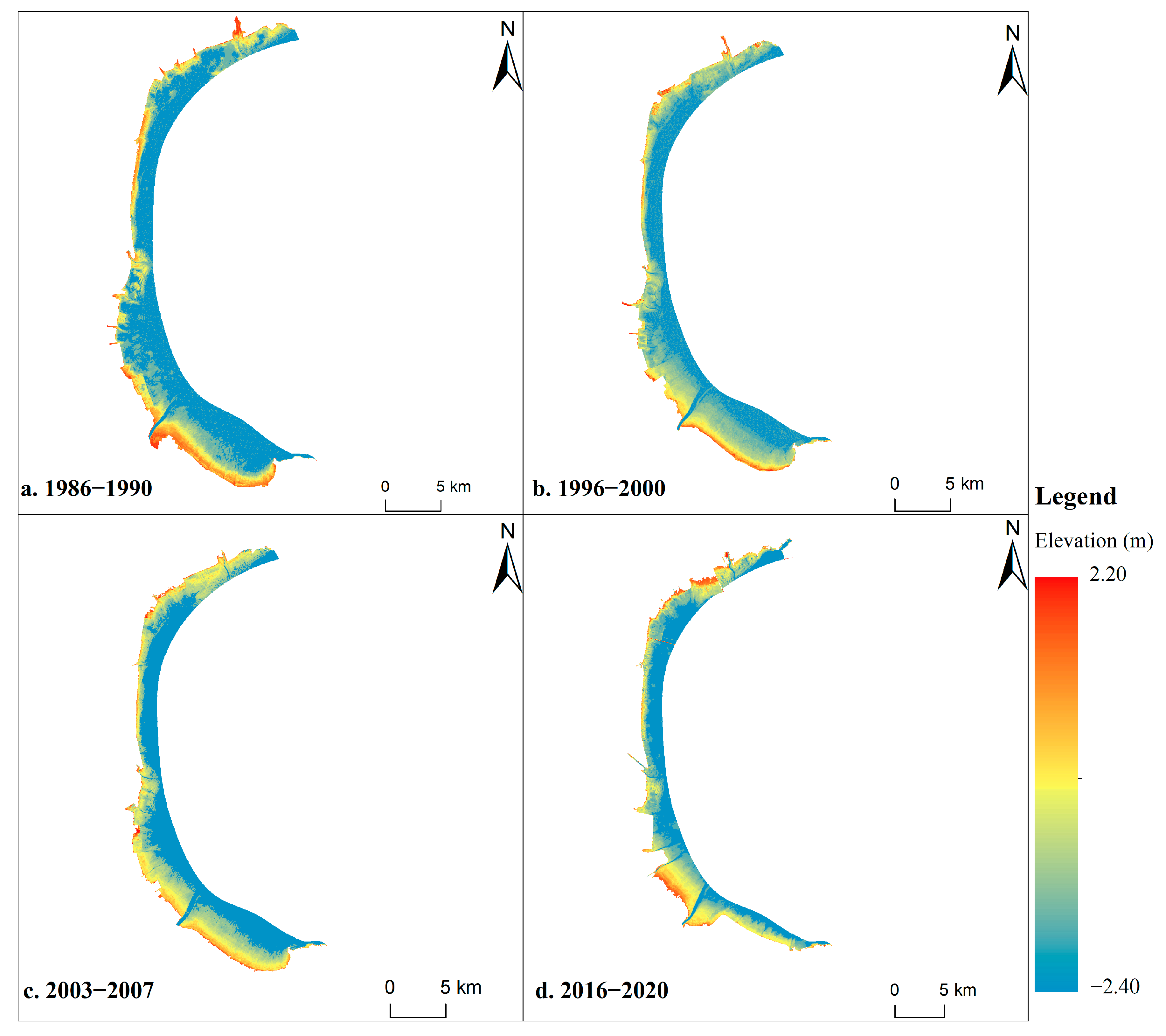
4.3. Analysis of Tidal Flats for Siltation

Figure 6 shows the inversion results of the topography of the beach and tidal flats in Haizhou Bay from 1996 to 2020, and the topography of the beach and tidal flats has evolved due to the influences of natural and anthropogenic factors. The northern part of Haizhou Bay shows erosion followed by siltation during 1986–2020, the central part of Haizhou Bay shows erosion, and the southern part of Haizhou Bay also shows siltation. The rivers in the north and south of Haizhou Bay were the main causes of siltation, while erosion occurred in the central part of Haizhou Bay due to the reduction in sediment sources, especially after the construction of dykes. In the southern part of Haizhou Bay, siltation was more pronounced in the south due to large-scale reclamation projects, while the tidal flats of the beaches in the reclaimed area were reduced in a large area. The data provided in this study can help to further study the evolution of human-acquired sediment transport in Haizhou Bay, where human reclamation activities are an important influence on the alteration of tidal flats and siltation in the area.

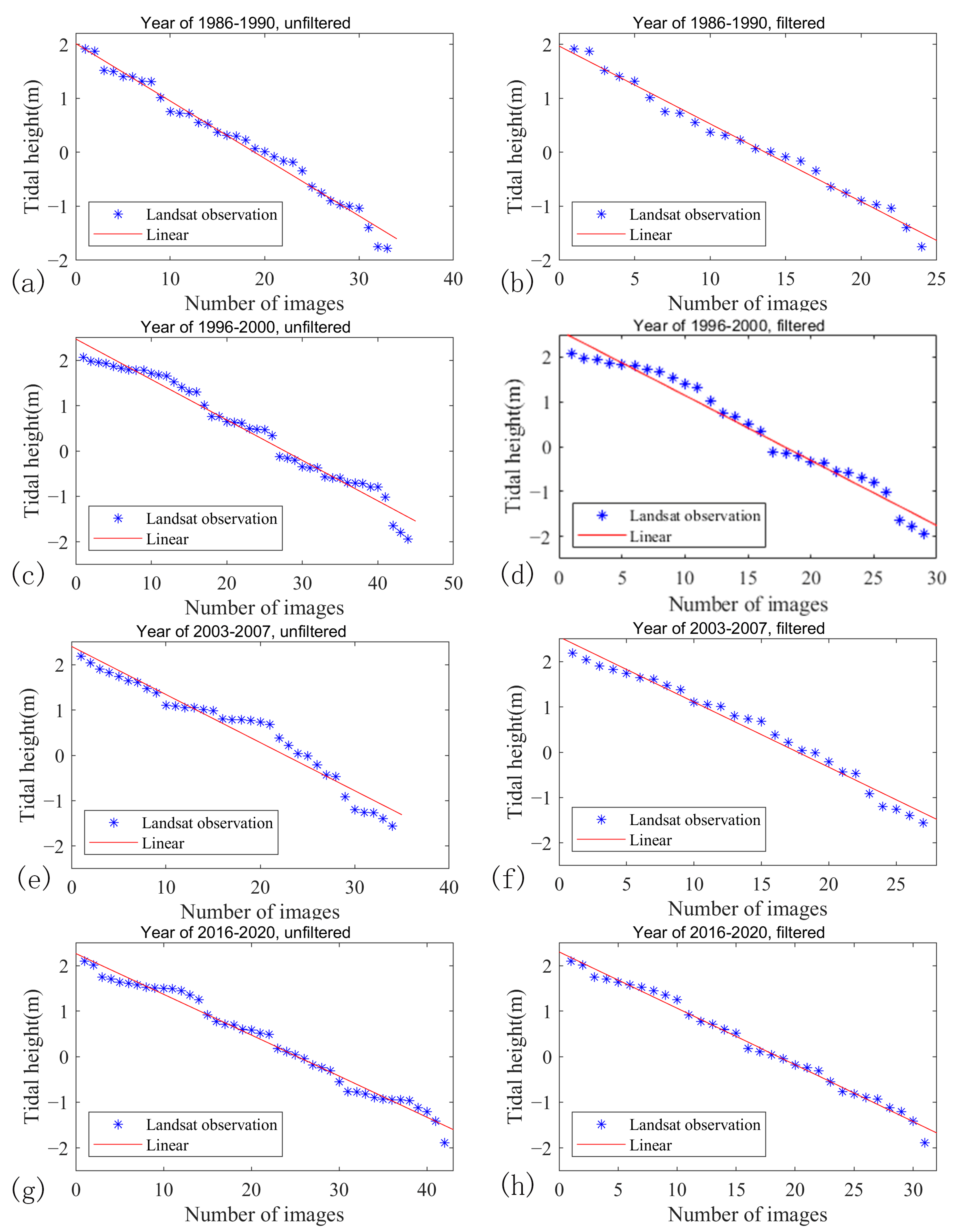
4.4. Impact of Screening Remote Sensing Imagery

As shown in Figure 7a,c,e,g show the distribution information of the tidal heights of the images before screening, and Figure 7b,d,f,h show the distribution of the tidal heights after screening. The tide level distribution characteristics of the available images at the four time points are different, but all of them exist at certain tide heights. There are multiple remote sensing images with relatively close elevations, which affects the true inundation frequency of the images, and undoubtedly weakens the advantages of the formulae applied in the inundation frequency method. After screening remote sensing images with intervals less than 1/n m, it can be seen that the distribution of the tide levels is more uniform, which is conducive to the inversion of beach topography using the linear formula.
The ideal situation for the inversion of beach topography is to have consistent intervals between the tidal heights of neighbouring images, with the size of the intervals being 1/n m. We compared and analysed the differences between using all the images and the screened images with the ideal condition and calculated the deviations of the results of the inversion in the ideal condition from the tide level of the actual image. The results are shown in Table 1 and Table 2, which show that the deviation from the ideal condition after screening is significantly reduced and that the root mean square error is reduced by 3–7 cm compared to with using all available remote sensing images at all time periods, indicating the feasibility of this method.

5. Discussion

5.1. Uncertainty Analysis

The development of a less subjective and automated process is essential for analysing complete data time series, which provides a basis for monitoring changes in beach tidal flat topography and studying potential natural and anthropogenic drivers [13]. In this study, human subjective factors were reduced in terms of water and land segmentation the tide level screening of similar remote sensing images, and elevation inversion. We demonstrated the feasibility of using Landsat TM/ETM+/OLI images and the GEE cloud computing platform to construct tidal flat topographies for coastal areas at a spatial resolution of 30 m. The accuracy validation results of the inversion show the reliability of this method in constructing a beach tidal flat topography, but the long observation interval causes uncertainty in the variation of the beach tidal flat topography and the tide level information, which can interfere with the influence of the beach tidal flat topography elevation. At present, only Landsat remote sensing images can monitor tidal flats at a long time scale, with a revisitation period of 16 days, and about 22 remote sensing images can be obtained in a year. However, there is not enough remote sensing imagery available within one year due to cloud cover, so the inundation frequency method when using Landsat imagery generally uses remote sensing imagery within five years [15,39]. The morphology of tidal flats inevitably changes over five years. However, this study requires a certain number of remote sensing images to ensure the vertical accuracy of the tidal flat construction and the coverage of the tide level, which is a trade-off problem. Although spatial interpolation can be used to resolve these discontinuities, as in the waterline method, the resulting DEMs are much less representative of actual surface elevations. The intertidal topography of most estuaries or bays does not change significantly in the short term [16,40], with the topography of the Yangtze River estuary varying by approximately 10–20 cm per year [41]. The relatively small size of the rivers in this study area compared to the mouth of the Yangtze River is likely to result in even less variation in topography year to year, so the average topography over a five-year period reflects the tidal flat elevation to some extent.
In order to assess the change in the beach tidal flats in Haizhou Bay over five years, we selected remote sensing imagery available for each of the years 2016–2020 to construct the topography of the beach tidal flats for each year. Profile 1 was selected to assess the inter-annual change in the beach tidal flats, using the inverted elevation at Section 1 for each year minus the measured elevation of profile 1 in 2016, and the mean value of the interpolated values for each year was calculated, and the results are shown in Figure 8. Without considering the effect of the insufficient number of remote sensing images on the accuracy of the results, it can be seen that the results for 2016 were closest to the measured one, while the results for 2020 had the largest difference. The black dashed line in the figure shows the average elevation change between five years, and its mean value is 0.14 m, indicating that the topography did not change much during the five years, which also shows that the average beach and tidal flat topography constructed from five years of remotely sensed imagery can roughly reflect the actual situation of the tidal flats. The topography of tidal flats is highly variable due to human reclamation projects, which often cause the topography of tidal flats to increase and siltation to occur around them. The topography constructed using the inundation frequency method is the average of five years, which will make the results of the topography of the reclaimed area low. Therefore, to meet the requirement of the number of remote sensing images, the inundation frequency method is not suitable for areas with large topographic changes.
Tide level information is also an important factor affecting the accuracy of the results, and the assumptions underpinning our approach are that the results of the TPXO9 tidal simulation allow us to map the moment of acquisition of the image to the tide level, and that the water/non-water variations are related only to the tide [13]. However, the tidal model is limited in the accuracy of the tide level simulation by nearshore topography and weather. We do not have enough measured data to verify the accuracy of the tide level simulation, but the accuracy of the inversion of the tidal terrain of the tidal flats was improved after screening some remote sensing images with close tidal heights, which indicates the reliability of the tide level simulation. Although the inundation frequency method is not overly dependent on the tide level, the optimisation method proposed in this study needs to incorporate the tide level information, and when the tide information is inaccurate, the culled image tide levels are not necessarily uniformly distributed, thus increasing the error in the construction of tidal flats topography.
Indeed, the selection of interval 1/n m as the culling interval in this study was not necessarily the optimal interval, but the idea proposed in this study can be learnt from; by culling part of the images with similar intervals, the distribution of the water level can be constructed to be more uniform, to improve the inversion accuracy of the tidal flats topography. In addition, exploring more appropriate land and water segmentation methods will also improve the inversion accuracy of tidal flat topography.

5.2. Impact of Dense Distribution of Remote Sensing Imagery

The inundation frequency method is similar to the Monte Carlo method, which is based on the calculation method of “random numbers”. The selected remote sensing images can be regarded as random, and as the number of images increases, the distribution of the selected tide levels becomes more uniform.. Then, the accuracy of the inversion of the tidal flat topography will be more accurate. In Section 5.1, we used the remote sensing images of a single year to analyse the inter-annual variation in beach tidal flat topography, and the results showed that the average value of the overall variation during a five-year time period was higher than that of the measured topography in 2016, while the results of the validation section in Section 4.1 showed that the inverted elevation was lower than that of the measured elevation, which may be due to a lack of remote sensing images for a single year, and the uneven distribution of the water level at the time of the acquisition. However, the use of all remote sensing images in a five-year time period can satisfy the quantity requirement, but the problem of uneven water level distribution still needs to be solved: how to assess the impact caused by the concentration of remote sensing images corresponding to the distribution of the water level? Firstly, the vertical concentration of the water level in the image is manifested in the lateral direction by a sharp change in the slope of the tidal flat edge of the beach in the water level inversion of the concentration of the water level distribution in the remotely sensed image. If part of the concentrated water level is biased upward, it will cause the inversion profile to be concave downward and lower than the actual elevation; if part of the concentrated water level is biased downward, it will cause the inversion profile to be convex upward and higher than the actual elevation. Secondly, as the number of remote sensing images increases, and not all of them are concentrated in a certain water level, it will weaken the effect of the water level distribution concentration of remote sensing images. This is because number of remotely sensed images and the randomness of the images corresponding to the water level increase, making the remotely sensed water level tend to be uniformly distributed, e.g., the combination of an upwardly concentrated water level and downwardly concentrated water level counteracts the effects of downward concavity and upward convexity. Finally, although inverting as many images as possible to the terrain can reduce the effect of the image water level distribution concentration, it is not the optimal method. By filtering out remote sensing images with water level intervals less than 1/n m and eliminating those with overly concentrated distributions, the water level distribution can be made more homogeneous, thus improving the inversion accuracy of the tidal flat topography of the beach.

6. Conclusions

In this study, the historical evolution of the beach tidal flats in Haizhou Bay was analysed using Landsat images and the global tidal model TPXO9, based on the inundation frequency method. Haizhou Bay is a bay close to the city; its coastal tidal flats have changed considerably due to artificial reclamation and aquaculture. The shoreline in the southern and central parts of Haizhou Bay has changed significantly, while the central part has remained basically stable; tidal flats show siltation in the southern and northern parts and erosion in the central part of the bay. In this study, we considered the effect of the over-concentration of acquired images at some water levels, and screened out some images with close water levels according to the number of acquired images. The results show that the error in the construction of the tidal flat topography of the beach can be reduced by eliminating images with close water levels. In analysing the comparison area selected in the south, it was found that the DEM constructed using all remote sensing imagery was even more skewed with the measured results.
Meanwhile, this study also explored the reasonableness of selecting a five-year time interval and the effect of an uneven distribution of water levels in the images. The topography of tidal flats constructed over a five-year period using remote sensing data from a single year was found to have a mean change in tidal flat topography of 0.14 m, which is within an acceptable range. The effect of the concentration of the image water level distribution on the inversion results can be weakened when a sufficient number of images are used, but the accuracy of the inversion of the topography of the tidal flats can be further improved by filtering out some of the remotely sensed images that are close to the water level. The method of this study is reproducible, and the data are easy to obtain, and the application of this method in other coastal areas around the world can enrich the coastal topographic data and provide technical support for the protection and management of tidal flats.

Author Contributions

S.M.: Conceptualisation, Methodology, Validation, Investigation, Writing—Original Draft, Visualisation, Writing—Review and Editing. N.W.: Conceptualisation, Methodology, Validation, Investigation, Writing—Original Draft, Visualisation, Writing—Review and Editing. L.Z.: Resources, Conceptualisation, Methodology, Validation, Investigation, Writing—Original Draft, Visualisation, Writing—Review and Editing. J.Y.: Writing—Review and Editing. X.C.: Data Curation. Y.C.: Data Curation. All authors have read and agreed to the published version of the manuscript.

Funding

This study was funded by Key Laboratory of Ocean Space Resource Management Technology, MNR (KF-2023-111), and the National Natural Science Funds of China (42076010).

Data Availability Statement

Data will be made available upon request.

Acknowledgments

Thanks to GEE for providing the data processing platform. The authors would like to express their sincere thanks to Bao Xianwen, Mou Xiujuan and Li Xiuren for their suggestions and support during the research process.

Conflicts of Interest

The authors declare that they have no known competing financial interests or personal relationships that could have appeared to influence the work reported in this paper.

References

  1. Murray, N.J.; Ma, Z.; Fuller, R.A. Tidal Flats of the Yellow Sea: A Review of Ecosystem Status and Anthropogenic Threats. Austral Ecol. 2015, 40, 472–481. [Google Scholar] [CrossRef]
  2. Nienhuis, J.H.; Ashton, A.D.; Edmonds, D.A.; Hoitink, A.J.F.; Kettner, A.J.; Rowland, J.C.; Törnqvist, T.E. Global-Scale Human Impact on Delta Morphology Has Led to Net Land Area Gain. Nature 2020, 577, 514–518. [Google Scholar] [CrossRef] [PubMed]
  3. Guo, H.; Cai, Y.; Yang, Z.; Zhu, Z.; Ouyang, Y. Dynamic Simulation of Coastal Wetlands for Guangdong-Hong Kong-Macao Greater Bay Area Based on Multi-Temporal Landsat Images and FLUS Model. Ecol. Indic. 2021, 125, 107559. [Google Scholar] [CrossRef]
  4. Wang, X.; Xiao, X.; Zou, Z.; Chen, B.; Ma, J.; Dong, J.; Doughty, R.B.; Zhong, Q.; Qin, Y.; Dai, S.; et al. Tracking Annual Changes of Coastal Tidal Flats in China during 1986–2016 through Analyses of Landsat Images with Google Earth Engine. Remote Sens. Environ. 2020, 238, 110987. [Google Scholar] [CrossRef] [PubMed]
  5. Barbier, E.B.; Hacker, S.D.; Kennedy, C.; Koch, E.W.; Stier, A.C.; Silliman, B.R. The Value of Estuarine and Coastal Ecosystem Services. Ecol. Monogr. 2011, 81, 169–193. [Google Scholar] [CrossRef]
  6. Zohary, T.; Gasith, A. The Littoral Zone. In Lake Kinneret: Ecology and Management; Zohary, T., Sukenik, A., Berman, T., Nishri, A., Eds.; Aquatic Ecology Series; Springer: Dordrecht, The Netherlands, 2014; pp. 517–532. ISBN 978-94-017-8944-8. [Google Scholar]
  7. Yao, H. Characterizing Landuse Changes in 1990–2010 in the Coastal Zone of Nantong, Jiangsu Province, China. Ocean Coast. Manag. 2013, 71, 108–115. [Google Scholar] [CrossRef]
  8. Zhao, Y.; Liu, Q.; Huang, R.; Pan, H.; Xu, M. Recent Evolution of Coastal Tidal Flats and the Impacts of Intensified Human Activities in the Modern Radial Sand Ridges, East China. Int. J. Environ. Res. Public Health 2020, 17, 3191. [Google Scholar] [CrossRef] [PubMed]
  9. Jia, M.; Wang, Z.; Mao, D.; Ren, C.; Wang, C.; Wang, Y. Rapid, Robust, and Automated Mapping of Tidal Flats in China Using Time Series Sentinel-2 Images and Google Earth Engine. Remote Sens. Environ. 2021, 255, 112285. [Google Scholar] [CrossRef]
  10. Zhao, C.; Qin, C.-Z.; Teng, J. Mapping Large-Area Tidal Flats without the Dependence on Tidal Elevations: A Case Study of Southern China. ISPRS J. Photogramm. Remote Sens. 2020, 159, 256–270. [Google Scholar] [CrossRef]
  11. Xu, N.; Ma, Y.; Yang, J.; Wang, X.H.; Wang, Y.; Xu, R. Deriving Tidal Flat Topography Using ICESat-2 Laser Altimetry and Sentinel-2 Imagery. Geophys. Res. Lett. 2022, 49, e2021GL096813. [Google Scholar] [CrossRef]
  12. Ryu, J.-H.; Kim, C.-H.; Lee, Y.-K.; Won, J.-S.; Chun, S.-S.; Lee, S. Detecting the Intertidal Morphologic Change Using Satellite Data. Estuar. Coast. Shelf Sci. 2008, 78, 623–632. [Google Scholar] [CrossRef]
  13. Sagar, S.; Roberts, D.; Bala, B.; Lymburner, L. Extracting the Intertidal Extent and Topography of the Australian Coastline from a 28year Time Series of Landsat Observations. Remote Sens. Environ. 2017, 195, 153–169. [Google Scholar] [CrossRef]
  14. Lijun, Y.; Yao, X.; Jie, J.; Yixiang, C.; Yan, G.; Sentong, Z. Remote Sensing Method for Extracting Topographic Information on Tidal Flats Using Spatial Distribution Features. Mar. Geod. 2021, 44, 408–431. [Google Scholar] [CrossRef]
  15. Tseng, K.-H.; Kuo, C.-Y.; Lin, T.-H.; Huang, Z.-C.; Lin, Y.-C.; Liao, W.-H.; Chen, C.-F. Reconstruction of Time-Varying Tidal Flat Topography Using Optical Remote Sensing Imageries. ISPRS J. Photogramm. Remote Sens. 2017, 131, 92–103. [Google Scholar] [CrossRef]
  16. Chen, C.; Zhang, C.; Tian, B.; Wu, W.; Zhou, Y. Tide2Topo: A New Method for Mapping Intertidal Topography Accurately in Complex Estuaries and Bays with Time-Series Sentinel-2 Images. ISPRS J. Photogramm. Remote Sens. 2023, 200, 55–72. [Google Scholar] [CrossRef]
  17. Choi, J.-K.; Ryu, J.-H.; Lee, Y.-K.; Yoo, H.-R.; Woo, H.J.; Kim, C.H. Quantitative Estimation of Intertidal Sediment Characteristics Using Remote Sensing and GIS. Estuar. Coast. Shelf Sci. 2010, 88, 125–134. [Google Scholar] [CrossRef]
  18. Pan, H.; Jia, Y.; Zhao, D.; Xiu, T.; Duan, F. A Tidal Flat Wetlands Delineation and Classification Method for High-Resolution Imagery. ISPRS Int. J. Geo-Inf. 2021, 10, 451. [Google Scholar] [CrossRef]
  19. Liu, Y.; Huang, H.; Qiu, Z.; Fan, J. Detecting Coastline Change from Satellite Images Based on Beach Slope Estimation in a Tidal Flat. Int. J. Appl. Earth Obs. Geoinf. 2013, 23, 165–176. [Google Scholar] [CrossRef]
  20. Bell, P.S.; Bird, C.O.; Plater, A.J. A Temporal Waterline Approach to Mapping Intertidal Areas Using X-Band Marine Radar. Coast. Eng. 2016, 107, 84–101. [Google Scholar] [CrossRef]
  21. Salameh, E.; Frappart, F.; Turki, I.; Laignel, B. Intertidal Topography Mapping Using the Waterline Method from Sentinel-1 & -2 Images: The Examples of Arcachon and Veys Bays in France. ISPRS J. Photogramm. Remote Sens. 2020, 163, 98–120. [Google Scholar] [CrossRef]
  22. Tong, S.S.; Deroin, J.P.; Pham, T.L. An Optimal Waterline Approach for Studying Tidal Flat Morphological Changes Using Remote Sensing Data: A Case of the Northern Coast of Vietnam. Estuar. Coast. Shelf Sci. 2020, 236, 106613. [Google Scholar] [CrossRef]
  23. Yang, Z.; Wang, L.; Sun, W.; Xu, W.; Tian, B.; Zhou, Y.; Yang, G.; Chen, C. A New Adaptive Remote Sensing Extraction Algorithm for Complex Muddy Coast Waterline. Remote Sens. 2022, 14, 861. [Google Scholar] [CrossRef]
  24. Zhang, M.; Wu, W.T.; Wang, X.Q.; Sun, Y. Topographic retrieval of the tidal flats in the Yangtze Estuary based on the dynamic tidal submergence. J. Geo-Inf. Sci. 2022, 24, 583–596. [Google Scholar] [CrossRef]
  25. Ai, B.; Wang, P.; Yang, Z.; Tian, Y.; Liu, D. Spatiotemporal Dynamics Analysis of Aquaculture Zones and Its Impact on Green Tide Disaster in Haizhou Bay, China. Mar. Environ. Res. 2023, 183, 105825. [Google Scholar] [CrossRef] [PubMed]
  26. Iwamura, T.; Fuller, R.A.; Possingham, H.P. Optimal Management of a Multispecies Shorebird Flyway under Sea-Level Rise. Conserv. Biol. 2014, 28, 1710–1720. [Google Scholar] [CrossRef] [PubMed]
  27. Egbert, G.D.; Erofeeva, S.Y. Efficient Inverse Modeling of Barotropic Ocean Tides. J. Atmos. Ocean. Technol. 2002, 19, 183–204. [Google Scholar] [CrossRef]
  28. Xu, H. Modification of Normalised Difference Water Index (NDWI) to Enhance Open Water Features in Remotely Sensed Imagery. Int. J. Remote Sens. 2006, 27, 3025–3033. [Google Scholar] [CrossRef]
  29. Jain, A.; Ramakrishnan, R.; Thomaskutty, A.V.; Agrawal, R.; Rajawat, A.S.; Solanki, H. Topography and Morphodynamic Study of Intertidal Mudflats along the Eastern Coast of the Gulf of Khambhat, India Using Remote Sensing Techniques. Remote Sens. Appl. Soc. Environ. 2022, 27, 100798. [Google Scholar] [CrossRef]
  30. Mghaiouini, R.; Benzbiria, N.; Belghiti, M.E.; Belghiti, H.E.; Monkade, M.; El bouari, A. Optical Properties of Water under the Action of the Electromagnetic Field in the Infrared Spectrum. Mater. Today Proc. 2020, 30, 1046–1051. [Google Scholar] [CrossRef]
  31. Alam, S.M.R.; Hossain, M.S. A Rule-Based Classification Method for Mapping Saltmarsh Land-Cover in South-Eastern Bangladesh from Landsat-8 OLI. Can. J. Remote Sens. 2021, 47, 356–380. [Google Scholar] [CrossRef]
  32. Hossain, M.S.; Hashim, M.; Bujang, J.S.; Zakaria, M.H.; Muslim, A.M. Assessment of the Impact of Coastal Reclamation Activities on Seagrass Meadows in Sungai Pulai Estuary, Malaysia, Using Landsat Data (1994–2017). Int. J. Remote Sens. 2019, 40, 3571–3605. [Google Scholar] [CrossRef]
  33. Colditz, R.R.; Troche Souza, C.; Vazquez, B.; Wickel, A.J.; Ressl, R. Analysis of Optimal Thresholds for Identification of Open Water Using MODIS-Derived Spectral Indices for Two Coastal Wetland Systems in Mexico. Int. J. Appl. Earth Obs. Geoinf. 2018, 70, 13–24. [Google Scholar] [CrossRef]
  34. Li, K.; Xu, T.; Xi, J.; Jia, H.; Gao, Z.; Sun, Z.; Yin, D.; Leng, L. Multi-Factor Analysis of Algal Blooms in Gate-Controlled Urban Water Bodies by Data Mining. Sci. Total Environ. 2021, 753, 141821. [Google Scholar] [CrossRef] [PubMed]
  35. Otsu, N. A Threshold Selection Method from Gray-Level Histograms. IEEE Trans. Syst. Man Cybern. 1979, 9, 62–66. [Google Scholar] [CrossRef]
  36. Dong, Z.; Wang, G.; Amankwah, S.O.Y.; Wei, X.; Hu, Y.; Feng, A. Monitoring the Summer Flooding in the Poyang Lake Area of China in 2020 Based on Sentinel-1 Data and Multiple Convolutional Neural Networks. Int. J. Appl. Earth Obs. Geoinf. 2021, 102, 102400. [Google Scholar] [CrossRef]
  37. Gong, Z.; Wang, Q.; Guan, H.; Zhou, D.; Zhang, L.; Jing, R.; Wang, X.; Li, Z. Extracting Tidal Creek Features in a Heterogeneous Background Using Sentinel-2 Imagery: A Case Study in the Yellow River Delta, China. Int. J. Remote Sens. 2020, 41, 3653–3676. [Google Scholar] [CrossRef]
  38. Tsai, Y.-L.S.; Tseng, K.-H. Monitoring Multidecadal Coastline Change and Reconstructing Tidal Flat Topography. Int. J. Appl. Earth Obs. Geoinf. 2023, 118, 103260. [Google Scholar] [CrossRef]
  39. Wang, Z.; Gao, Z.; Jiang, X. Analysis of the Evolution and Driving Forces of Tidal Wetlands at the Estuary of the Yellow River and Laizhou Bay Based on Remote Sensing Data Cube. Ocean Coast. Manag. 2023, 237, 106535. [Google Scholar] [CrossRef]
  40. Alam, S.M.R.; Hossain, M.S. Using a Water Index Approach to Mapping Periodically Inundated Saltmarsh Land-Cover Vegetation and Eco-Zonation Using Multi-Temporal Landsat 8 Imagery. J Coast Conserv. 2024, 28, 1–23. [Google Scholar] [CrossRef]
  41. Chen, C.; Zhang, C.; Wu, W.; Jiang, W.; Tian, B.; Zhou, Y. Application of UAV-Based Photogrammetry without Ground Control Points in Quantifying Intertidal Mudflat Morphodynamics. In Proceedings of the IGARSS 2022—2022 IEEE International Geoscience and Remote Sensing Symposium, Kuala Lumpur, Malaysia, 17–22 July 2022; pp. 7767–7770. [Google Scholar]
Figure 1. The geographical location of the study area in Haizhou Bay. The red frame in (a) is approximate location of the study area and the blue line in (b) is the study shore section.
Remotesensing 16 00685 g001
Figure 2. Temporal distribution of Landsat images in Haizhou Bay. (a) shows all the available remote sensing image sequences and (b) shows the remote sensing image sequences after optimisation. The blue dots indicate the corresponding tidal heights at the moment of Landsat imaging, and the green and red lines represent the mean high tide and mean low tide, respectively.
Remotesensing 16 00685 g002
Figure 3. Workflow of this study. MNDWI is “Modified Normalised Difference Water Index”.
Remotesensing 16 00685 g003
Figure 4. Profile location and accuracy verification results: (a) shows the topography of the southern part of Haijhou Bay from 2016 to 2020, and the purple and blue lines are accuracy-verified profiles. (b,c) show the results of the accuracy verification, black and red colours indicate the validation results for images filtered and unfiltered, respectively.
Remotesensing 16 00685 g004
Figure 5. Comparison of the results of the optimised inundation frequency method: (a) shows a satellite image of the south side of the study area, with a red box showing the comparison area. The green boxes in (bd) show the areas where the optimisation is more pronounced. (e,f) show the difference between the unfiltered and measured terrain and the filtered difference, respectively.
Remotesensing 16 00685 g005
Figure 6. Digital elevation models for four time periods in Haizhou Bay: (ad) show the topography constructed from 1986 to 1990, 1996 to 2000, 2003 to 2007 and 2016 to 2020, respectively.
Remotesensing 16 00685 g006
Figure 7. Tidal heights corresponding to the order of satellite images acquired for each period. The blue asterisk is the water level of the tide level image; the red line is the linear fit line. And (a,c,e,g) show the change in the water level of the image before the optimisation method was applied, and (b,d,f,h) shows the change in the water level of the image after the optimisation method was applied.
Remotesensing 16 00685 g007
Figure 8. Change in beach elevation from 2016 to 2020 from an average deviation of the 2016 measured topography. The blue dashed line shows the change in the average deviation, and the black dotted line shows the average deviation over the five years.
Remotesensing 16 00685 g008
Table 1. Deviation from ideal after filtering.
PeriodMaximum Deviation
(cm)
Minimum Deviation
(cm)
Average Deviation
(cm)
RMSE (cm)
1986–199020.70−31.97−08.2617.77
1996–20000−67.35−35.3340.86
2003–20077.25−51.57−21.8627.40
2016–20208.16−42.88−21.1824.95
Table 2. Deviation from ideal without filtering.
PeriodMaximum Deviation
(cm)
Minimum Deviation
(cm)
Average Deviation
(cm)
RMSE (cm)
1986–199016.75−43.76−13.4820.74
1996–20000−77.47−39.7444.53
2003–20079.44−76.93−23.2834.25
2016–202015.29−52.90−22.9928.46
Disclaimer/Publisher’s Note: The statements, opinions and data contained in all publications are solely those of the individual author(s) and contributor(s) and not of MDPI and/or the editor(s). MDPI and/or the editor(s) disclaim responsibility for any injury to people or property resulting from any ideas, methods, instructions or products referred to in the content.

