Developing a Multi-Scale Convolutional Neural Network for Spatiotemporal Fusion to Generate MODIS-like Data Using AVHRR and Landsat Images

Abstract

Remote sensing data are becoming increasingly important for quantifying long-term changes in land surfaces. Optical sensors onboard satellite platforms face a tradeoff between temporal and spatial resolutions. Spatiotemporal fusion models can produce high spatiotemporal data, while existing models are not designed to produce moderate-spatial-resolution data, like Moderate-Resolution Imaging Spectroradiometer (MODIS), which has moderate spatial detail and frequent temporal coverage. This limitation arises from the challenge of combining coarse- and fine-spatial-resolution data, due to their large spatial resolution gap. This study presents a novel model, named multi-scale convolutional neural network for spatiotemporal fusion (MSCSTF), to generate MODIS-like data by addressing the large spatial-scale gap in blending the Advanced Very-High-Resolution Radiometer (AVHRR) and Landsat images. To mitigate the considerable biases between AVHRR and Landsat with MODIS images, an image correction module is included into the model using deep supervision. The outcomes show that the modeled MODIS-like images are consistent with the observed ones in five tested areas, as evidenced by the root mean square errors (RMSE) of 0.030, 0.022, 0.075, 0.036, and 0.045, respectively. The model makes reasonable predictions on reconstructing retrospective MODIS-like data when evaluating against Landsat data. The proposed MSCSTF model outperforms six other comparative models in accuracy, with regional average RMSE values being lower by 0.005, 0.007, 0.073, 0.062, 0.070, and 0.060, respectively, compared to the counterparts in the other models. The developed method does not rely on MODIS images as input, and it has the potential to reconstruct MODIS-like data prior to 2000 for retrospective studies and applications.

1. Introduction

Satellite remote sensing has been providing essential records of land surface and dynamics both synoptically and periodically for decades [1,2,3]. The long-term accumulations of remote sensing data have facilitated numerous applications in Earth system sciences and have enhanced our understanding of environmental changes [4,5]. Temporally and spatially continuous products are favorable for various applications on large geographic scales, such as land surface modeling and climate dynamics simulations [6,7,8,9].

Optical remote sensing data are extensively used, and such data often face a tradeoff between temporal coverage frequency and spatial resolution when the data come from a single sensor. Fine-spatial-resolution multispectral images, like Landsat (30 m) and Sentinel (10–20 m) images, capture abundant geometric and texture features of the land surface [10,11], while their revisiting frequencies are relatively low [12]. Coarse-spatial-resolution images, like Advanced Very-High-Resolution Radiometer (AVHRR) images, are advantageous in providing daily global coverage but are limited in capturing spatial details [13,14,15]. Moderate-spatial-resolution images, like the Moderate-Resolution Imaging Spectroradiometer (MODIS) images, possess both sufficient spatial resolution and daily temporal frequency [16,17,18]. MODIS products have good quality control and have accelerated a number of large-scale studies, such as land cover mapping [19,20] and carbon budget calculation [21,22]. Since data with similar characteristics to MODIS were not available before 2000, generating MODIS-like data prior to 2000 holds great value for scientific studies. One way to produce continuous retrospective MODIS-like data is to blend multi-source images, such as Landsat and AVHRR data, because they have been available since 1982 and have similar characteristics in some bands. It is necessary to consider the large spatial-scale gap between fine- and coarse-spatial-resolution data when generating retrospective MODIS-like data using Landsat and AVHRR data.

Spatiotemporal fusion methods are widely applied to synergize multi-source remote sensing images to generate continuous data with dense temporal stacks and high spatial resolution [23,24]. Gao et al. [25] presented a rule-based data fusion model called the spatial and temporal adaptive reflectance fusion model (STARFM), which blends MODIS and Landsat data based on similar neighbor pixels and estimates well in relative homogeneous regions. Numerous research endeavors have further been devoted to enhancing the modeling abilities in regions characterized by pronounced spatial heterogeneity [26,27]; however, they fail to predict abrupt changes. Zhu et al. [28] developed the feasible spatiotemporal data fusion model (FSDAF) that incorporates the linear unmixing approach and spatial interpolation and has shown advantages in capturing abrupt changes in land cover types. Shi et al. [24] proposed the reliable and adaptive spatiotemporal data fusion method (RASDF), incorporating a reliability index to reduce biases caused by sensor differences. Commonly used rule-based spatiotemporal fusion methods were mainly developed to produce fine-spatial-resolution data, such as Landsat or Sentinel data [29,30,31,32,33,34]. However, these methods have not attempted to generate moderate-spatial-resolution data utilizing both coarse- and fine-spatial-resolution images.

Deep learning models have been extensively tested for spatiotemporal fusion because of their powerful nonlinear mapping capability. Tan et al. [35] presented the deep convolutional spatiotemporal fusion network (DCSTFN), inspired by the temporal change hypothesis from STARTM, to integrate MODIS and Landsat data. Tan et al. [36] presented an enhanced DCSTFN (EDCSTFN) using a brand-new network architecture and a compound loss function, thus preventing the image blurring that occurs in the DCSTFN. To maintain the reliability of temporal predictions, Liu et al. [37] designed a two-stream spatiotemporal fusion network (StfNet) that accounts for temporal dependence and consistency. Some scholars have proposed multi-scale convolutional approaches that use various filter sizes to extract spatial information across different scales [38,39,40,41]. To enhance model efficiency, Chen et al. [42] additionally leveraged the dilated convolutional method to expand the filter’s field-of-view, thereby better capturing multi-scale features. Deep-learning-based spatiotemporal fusion models offer a potential solution for generating MODIS-like data [43,44,45,46], and it is necessary to improve current spatiotemporal fusion models to address the large spatial resolution gaps and reduce biases among images acquired from different sensors.

The development of spatiotemporal fusion methods to reconstruct MODIS-like data using AVHRR and Landsat images faces some challenges. Spatial-scale issues arise due to the substantial spatial resolution gap between AVHRR and Landsat data, which cannot be addressed by current spatiotemporal fusion models without prior resampling procedures. However, the resampling procedure that has been adopted in current data fusion models involves unrealistic artificial assumption and loses fine spatial details. The current models are typically designed to fuse MODIS and Landsat images with about 16 times resolution difference, and they can hardly handle AVHRR and Landsat images, which have a spatial resolution difference of approximately 192 times. While the existing multi-scale spatiotemporal fusion methods aim to broaden the model’s receptive field, they also face challenges in addressing such a significant spatial-scale gap. Furthermore, systematic deviations caused by the spectral response function, viewing zenith angle, geo-registration errors, and acquisition time inconsistency between AVHRR and Landsat with MODIS images may introduce uncertainties into the fusion process. The existing spatiotemporal fusion models aim to blend images obtained from two different sensors, and certain models, such as BiaSTF, RASDF, and LiSTF [33], are designed to mitigate systematic deviations between MODIS and Landsat data. The retrospective construction of MODIS-like data using AVHRR and Landsat images has to deal with biases that originate from three different sensors.

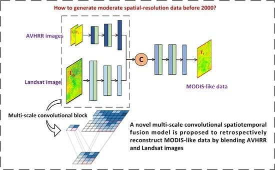
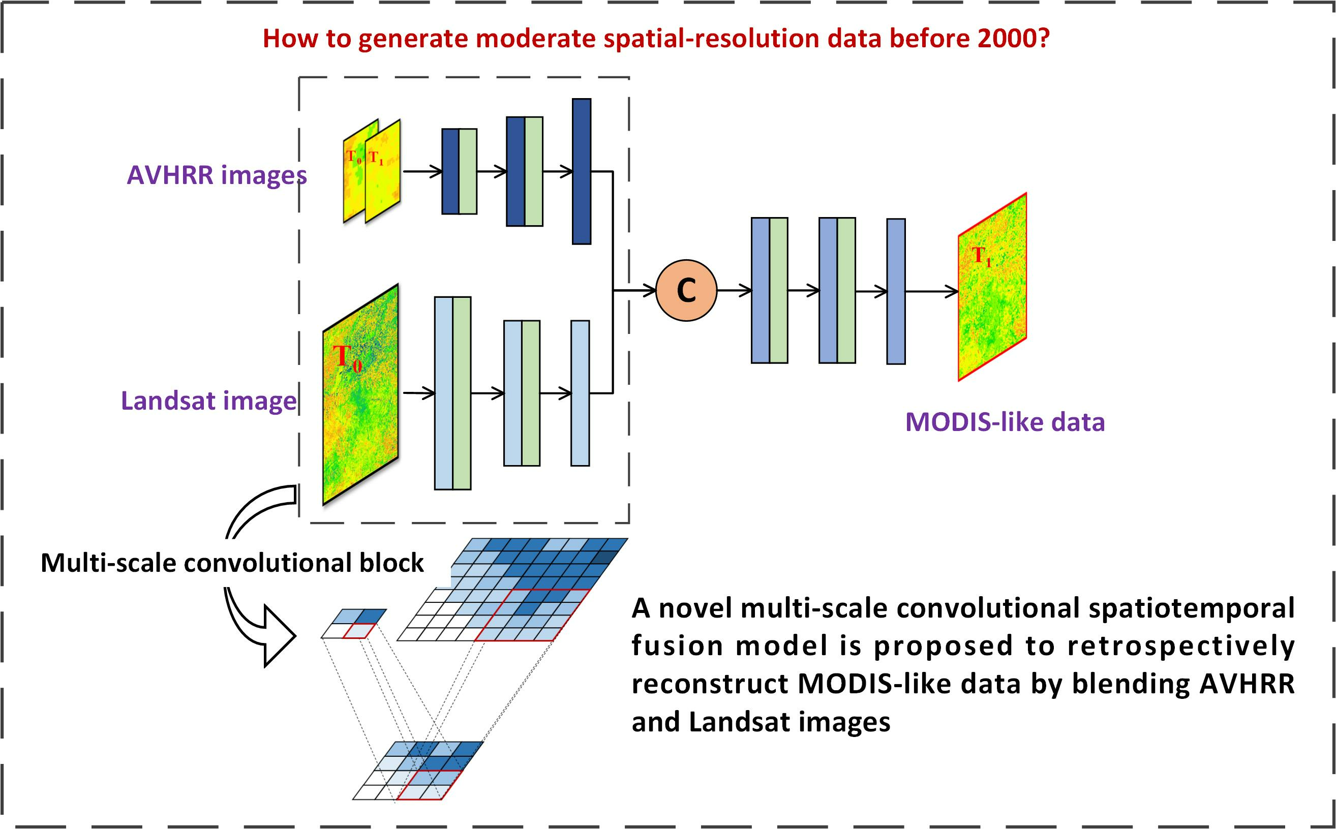
In this study, we proposed a novel model, called the multi-scale convolutional neural network for spatiotemporal fusion, to deal with spatial-scale gaps arising from the differences in spatial resolution between AVHRR and Landsat images by incorporating upscaling and downscaling approaches. We designed an image correction module before fusion and incorporated it into the model using deep supervision to alleviate the synthetic biases between the AVHRR and Landsat images with the MODIS data. Considering that AVHRR and Landsat images have been available since 1982, our model possesses the potential to reconstruct MODIS-like data prior to 2000 to facilitate retrospective research.

2. Study Materials

2.1. Study Regions

Our study evaluated the performance of spatiotemporal fusion methods in five landscapes characterized by strong spatial heterogeneity, mixed land cover type, and obvious seasonal changes across North America. The path/row combinations of the selected regions are 045/028, 042/034, 023/037, 052/017, and 014/028 in the Landsat Worldwide Reference System-2. These regions are located in The Dalles in Washington (WA), Mammoth Lake in California (CA), Greenville in Mississippi (MS), Nahanni Butte in the Northwest Territories (NT), and Sorel-Tracy in Quebec (QC) (Figure 1). WA predominantly comprises grasslands, evergreen needleleaf forests, and croplands. CA primarily consists of grasslands, woody savannas, and savannas. MS is predominantly characterized by croplands, mixed forests, and deciduous broadleaf forests and it is situated along the Mississippi River’s riverbanks. NT is primarily composed of evergreen needleleaf forests, woody savannas, and open shrublands. QC is primarily composed of mixed forests, croplands, and cropland/natural vegetation mosaics, with the Lac Saint-Pierre Lake and Saint Lawrence River situated at its center. Information regarding these regions is detailed in

Table 1. Information about the study regions.

Path	Row	Centered Town	State/Province	Code	Extent (km2)
045	028	The Dalles	Washington	WA	160 × 160
042	034	Mammoth Lake	California	CA	160 × 160
023	037	Greenville	Mississippi	MS	160 × 160
052	017	Nahanni Butte	Northwest Territories	NT	156 × 156
014	028	Sorel-Tracy	Quebec	QC	160 × 160

.

2.2. Remote Sensing Data

The fine-spatial-resolution images that we used are Landsat images, containing Landsat 5 Thematic Mapper (TM) and Landsat 8 Operational Land Imager (OLI) Collection 1 Tier 1 surface reflectance products. These images underwent atmospheric corrections and were calibrated for topographical correction using the UTM/WGS84 projection system (https://earthexplorer.usgs.gov (accessed on 25 October 2022)). Both Landsat 5 TM and Landsat 8 OLI are equipped with visible and NIR bands, providing a 30-m spatial resolution and 16-day temporal frequency. The MODIS images possess a moderate spatial resolution of 500 m and serve as the target outputs. We selected the MODIS Terra MOD09A1 Version 6 product, which supplies surface reflectance observation corrected for atmospheric contaminations (https://lpdaac.usgs.gov (accessed on 18 December 2023)). The MOD09A1 product comprises an 8-day composite of surface reflectance data, primarily consisting of 7 surface spectral reflectance bands and 2 quality control layers with a 500-m spatial resolution. The coarse-spatial-resolution AVHRR data are Version 5 Land Long-Term Data Record (LTDR) surface spectral reflectance products (AVH09C1) (https://ltdr.modaps.eosdis.nasa.gov (accessed on 20 December 2022)). The AVHRR product has been available from 1981 to the present and includes data for visible and NIR bands. We chose the daily AVH09C1 surface reflectance product provided by Wu et al. [14], which exhibits significantly better quality compared to the original 1.1-km images. Its spatial resolution is 0.05° (around five kilometers), and it was subjected to radiometric calibration and atmospheric correction.

We conducted spatiotemporal fusion experiments using vegetation index data. We opted to focus on the enhanced vegetation index 2 (EVI2) in this study when considering the constraints associated with commonly used vegetation indices such as the normalized difference vegetation index (NDVI) and the enhanced vegetation index (EVI) in certain scenarios. EVI2 is formulated to represent vegetation growth and aggregation situations by calculating from the red and near-infrared (NIR) bands [47]. Compared to NDVI, EVI2 is relatively insensitive to aerosol contamination and soil background and does not easily saturate in densely vegetated areas; therefore, it has a broader range of applications. EVI2 remains functionally equivalent to EVI without a blue band, thus it is suitable for use to analyze AVHRR data.

2.3. Data Preprocessing

The Landsat and AVHRR images were used from the time period spanning from 1981 to 2018, along with MODIS data from 2000 to 2018. Considering that the Landsat 7 images suffered from striping artifacts caused by a malfunction of the Scan Line Corrector (SLC) in the sensor, we used Landsat 5 and Landsat 8 images in the experiments. The cloud-free Landsat surface reflectance data with a cloud cover of less than 0.5% were selected from the Google Earth Engine (GEE) platform (https://earthengine.google.com (accessed on 25 December 2022)) in the five study regions, serving as the fine-spatial-resolution model input at the reference time. We acquired the available MODIS surface reflectance products for the five study areas to serve as the target data. The cloud-covered pixels within the Landsat and MODIS data were masked, and a linear interpolation method was applied along the time-series dimension to fill the few masked pixels. To ensure time consistency, the acquisition dates of the AVHRR images, which served as the inputs for both the reference and target times, were aligned with those of the corresponding Landsat images and MODIS images. The available cloud-free Landsat and AVHRR image pairs with the closest acquisition time to the target MODIS image were selected as the input data for the reference time. A total of 6, 5, 16, 11, and 16 samples from the available AVHRR–Landsat pairs after 2000 and their corresponding reference AVHRR–MODIS pairs were obtained for training purposes in the five regions, respectively. In the reconstruction of the retrospective MODIS-like data, a total of 37, 32, 38, 5, and 11 AVHRR–Landsat pairs were obtained from pre-2000 periods in the respective regions after excluding Landsat images with clouds. The reference and target times of the data in the retrospective reconstruction experiments are shown in

Table 2. The reference and target time of the model input and output in a retrospective reconstruction experiment for generating pre-2000 MODIS-like data in five study areas. The italicized text represents the target data.

Areas	Reference Time		Target Time		Reference Time		Target Time
	AVHRR	Landsat	AVHRR	Landsat	AVHRR	Landsat	AVHRR	Landsat
WA	1985/7/15	1985/7/15	1985/8/16	1985/8/16	1996/7/13	1996/7/13	1995/6/25	1995/6/25
CA	1985/8/27	1985/8/27	1985/8/11	1985/8/11	1994/3/13	1994/3/13	1994/2/9	1994/2/9
MS	1988/4/24	1988/4/24	1988/5/10	1988/5/10	1990/8/20	1990/8/20	1990/11/24	1990/11/24
NT	1993/4/1	1993/4/1	1984/7/29	1984/7/29	1995/8/13	1995/8/13	1995/8/13	1995/8/13
QC	1991/5/20	1991/5/20	1992/3/3	1992/3/3	1992/3/3	1992/3/3	1993/8/29	1993/8/29

, and those in the simulated experiments are shown in

Table 3. The same as Table 2, but for a simulated experiment for generating post-2000 MODIS-like data. There are three main columns of time data. The first two columns are linked to the comparison between the fused results with MODIS and Landsat images in Section 4.2, necessitating the alignment of the target time with the acquisition times of both MODIS and Landsat images. The third column is associated with the comparison with other spatiotemporal fusion models and the module ablation in Section 4.3 and 4.4, where the target times coincide with the acquisition times of the MODIS images.

Areas	Reference Time		Target Time		Reference Time		Target Time		Reference Time		Target Time
	AVHRR	Landsat	AVHRR	MODIS	AVHRR	Landsat	AVHRR	MODIS	AVHRR	Landsat	AVHRR	MODIS
WA	2015/7/4	2015/7/4	2014/9/30	2014/9/30	2018/9/30	2018/9/30	2018/10/16	2018/10/16	2015/7/2	2015/7/2	2015/7/20	2015/7/20
CA	2014/9/14	2014/9/14	2014/8/29	2014/8/29	2016/9/21	2016/9/21	2018/9/06	2018/9/6	2004/8/27	2004/8/27	2001/9/14	2001/9/14
MS	2016/6/09	2016/6/09	2016/5/8	2016/5/8	2017/4/7	2017/4/7	2017/10/16	2017/10/16	2004/6/21	2004/6/21	2002/6/18	2002/6/18
NT	2014/4/15	2014/4/15	2013/8/29	2013/8/29	2014/8/5	2014/8/5	2014/4/15	2014/4/15	2013/8/30	2013/8/30	2012/7/3	2012/7/3
QC	2001/3/14	2001/3/14	2001/2/26	2001/2/26	2009/11/17	2009/11/17	2009/9/14	2009/9/14	2005/6/27	2005/6/27	2005/8/29	2005/8/29

. The AVHRR, MODIS, and Landsat images were spatially aligned by reprojecting them to the UTM/WGS84 projection system and were clipped to match the spatial extent. We resampled the AVHRR and Landsat images to 1/12th and 16 times the grid resolution of the MODIS data, respectively, using the cubic spline interpolation method. Consequently, the proposed model combined the inputs from an AVHRR and Landsat image pair at the reference time, along with an AVHRR image at the target time. The MODIS images at the target time were referred to as the target objects.

We selected the red (0.63–0.69 μm) and NIR (0.76–0.9 μm) bands from Landsat 5 images, while the corresponding wavelengths in the Landsat 8 images were 0.64–0.67 μm, and 0.85–0.88 μm, respectively. The red (0.62–0.67 μm) and NIR (0.84–0.88 μm) bands from the MODIS product were utilized. The red (0.58–0.68 μm) and NIR (0.73–1.00 μm) bands from the AVHRR data were also included. The wavelengths associated with these three datasets are comparable, with the Landsat data exhibiting the narrowest range of wavelengths and the AVHRR data featuring the longest range of wavelengths. The wavelengths of the corresponding bands in the Landsat 5 and Landsat 8 products differed, so we employed a random forest method to independently calibrate the red and NIR bands of Landsat 5 to ensure the alignment between the Landsat 5 and Landsat 8 data. Then, we calculated EVI2 based on the red and NIR bands and obtained the model inputs and targets as the AVHRR, Landsat, and MODIS EVI2 data.

3. Methods

3.1. MSCSTF

A multi-scale convolutional neural network for spatiotemporal fusion (hereafter referred to as MSCSTF) was proposed to generate MODIS-like data by blending the AVHRR and Landsat images. The model incorporates a multi-scale feature extraction approach to address the huge spatial-resolution gap between the AVHRR and Landsat images, and it introduces an image correction module to mitigate the synthetic biases between the AVHRR and Landsat and the MODIS data. Figure 2 shows an illustrative scheme of the MSCSTF structure. MSCSTF can be described using a generalized equation, as follows:

$${\mathrm{F}}_1=\mathrm{STF}(\mathrm{Correct}(\mathrm{Upscale}({\mathrm{L}}_0)),\mathrm{Downscale}(\mathrm{Correct}({\mathrm{A}}_0,{\mathrm{A}}_1)))$$

(1)

where F, L, and A denote the fused MODIS-like data, the Landsat images, and the AVHRR images, respectively. Here, 0 and 1 refer to the reference and target times, respectively. Upscale() and Downscale() denote the upscaling and downscaling approaches, respectively. Correct() denotes the image correction module. STF() refers to the deep learning spatiotemporal fusion module.

MSCSTF encompasses the following three modules: a multi-scale feature extraction module, an image correction module, and a spatiotemporal fusion module. The multi-scale feature extraction module includes Landsat feature upscaling and AVHRR feature downscaling approaches, and the image correction module contains Landsat-based correction and AVHRR-based correction approaches. The high-resolution Landsat data are first compressed to moderate-resolution features by means of Landsat feature upscaling and are then subjected to Landsat-based correction to reduce the biases between the Landsat and MODIS images. The AVHRR images underwent AVHRR-based correction to mitigate the deviations between the AVHRR and MODIS data, followed by downscaling to align with the MODIS data’s spatial resolution. The extracted AVHRR and Landsat features were concatenated and fed into the spatiotemporal fusion module to generate fused MODIS-like data. MSCSTF is an end-to-end model where all modules are trained simultaneously to achieve an optimal model.

3.2. Multi-Scale Feature Extraction Module

There is an approximately 192-fold spatial-scale difference between the Landsat and AVHRR data, where the difference between Landsat and MODIS imagery is 16-fold, and 12-fold between AVHRR and MODIS data. Due to the complexity of spatial distribution, the differences in spatial detail among remote sensing datasets cannot be readily resolved using empirical interpolation methods. A multi-scale feature extraction module was incorporated by a learning way to address the spatial-scale issues between the Landsat and AVHRR images. By incorporating both the upscaling and downscaling methods, the model has the ability to construct nonlinear spatial pyramid mapping between fine- and coarse-resolution data, thereby better addressing spatial-scale issues and capturing moderate-resolution spatial details (Figure 3). During the upscaling stage, the stride-convolutional blocks captured fine-grained spatial details from the Landsat data and integrated them to align with the MODIS data’s spatial resolution. Transposed convolutional blocks were applied in the downscaling phase to unmix the spatial patterns of the coarse-resolution AVHRR features to moderate-resolution spatial features.

The upscaling approach encompasses three stride-convolutional blocks. The first two stride-convolutional blocks contain a stride-convolutional layer and an activation layer, while the last block comprises only a stride-convolutional layer. The downscaling technique consists of three transposed convolutional blocks, in which each of the first two blocks comprise a transposed convolutional layer and an activation layer, while the last block has a single transposed convolutional layer.

3.3. Image Correction Module

Correcting the biases between the images acquired from different sensors prior to the spatiotemporal fusion phase is essential to enhance the performance of spatiotemporal fusion. An image correction module was employed to alleviate the systematic biases between the AVHRR and Landsat images and the MODIS images using AVHRR-based correction and Landsat-based correction methods, respectively. The network incorporates the image correction module in a deep supervision way to achieve an end-to-end model.

Deep supervision is primarily applied in image classification to optimize the deep neural network and accelerate convergence [48,49]. Deep supervision adds an additional auxiliary classifier, i.e., loss function, with a companion objective for each branch in some intermediate hidden layers, aiding the weight adjustment of these layers.

For a learning-based neural network, we refer to $M$ as the total number of layers, and $W^{(m)}$ denotes the weight at the $m$ th hidden layer, while ${\omega }^{(m)}$ represents the weight of the $m$ th supervised hidden layer, distinguishing it from the normal layer. Specifically, for a conventional network, the weights for all layers can be denoted as $W=\{W^{(1)},\dots ,W^{(M-1)}\}$, along with the weight of the output layer ${\omega }^{(out)}$. The network’s objective function gives the following:

$$P(W)=L(W,{\omega }^{(out)})$$

(2)

where $L(W,{\omega }^{(out)})$ denotes the loss function determined by ${\omega }^{(out)}$, and ${\omega }^{(out)}$ depends on $W$.

As for the deep supervision network, where each intermediate layer is associated with a supervisor, the corresponding weights are given as follows: $\omega =\{{\omega }^{(1)},\dots ,{\omega }^{(M-1)}\}$. The summed companion objective function of all $M-1$ hidden layers can be interpreted as follows:

$$Q(W)={\displaystyle \sum _{m=1}^{M-1}{\alpha }_{m}l(W,{\omega }^{(m)})}$$

(3)

where $l(W,{\omega }^{(m)})$ and ${\alpha }_m$ are a companion loss function and a coefficient, respectively, of the $m$ th companion supervisor. The ground truth data for different supervisors are commonly consistent, and the ultimate objective function is compounded by the sum of each companion objective function and the last objective function and offer integrated supervision to improve the network’s performance. Thus, the overall objective function for a deep supervision network is as follows:

$$F(W)=P(W)+Q(W)$$

(4)

Differing from traditional deep supervision methods, the image correction module in MSCSTF has two independent companion supervisors with different ground truth targets in the AVHRR-based correction and Landsat-based correction phases (Figure 4). The target data in the AVHRR-based correction phase are the resampled low-resolution MODIS images at both the reference and target times, and that in Landsat-based correction is a moderate-resolution MODIS image at the reference time. The objective functions for AVHRR- and Landsat-based corrections can be defined, respectively, as follows:

$$Q_A(W)=l(W,{\omega }^{(m_A)})$$

(5)

$$Q_L(W)=l(W,{\omega }^{(m_L)})$$

(6)

where $m_A$ and $m_L$ denote the number of layers for the supervisors of AVHRR- and Landsat-based corrections, respectively. The two correction networks independently adjust the weight parameters to mitigate the systematic biases between the AVHRR and Landsat inputs with their corresponding target MODIS data. The final objective function of the spatiotemporal fusion module is only for the output layer, as follows:

$$F_{fuse}(W)=P(W)$$

(7)

The AVHRR images at both the reference and target times were subjected to AVHRR-based correction, and the upscaled Landsat features were subjected to Landsat-based correction. Each image correction network comprises three convolutional blocks. The initial two blocks have identical compositions, encompassing convolutional and ReLU activation layers. The ultimate part diverges into two branches, in which a correction branch with one convolutional layer is constructed to adjust the trainable weights of the image correction network. The other branch is a backbone branch for transporting corrected high-level traits to the subsequent layer.

3.4. Loss Function

A compound loss function that combines structural and pixel penalty functions was implemented. Multi-scale structural similarity (MS-SSIM) [50] was used to calculate the structural loss, and the relative Charbonnier function [51] was employed for pixel loss.

$${\mathrm{L}}_{\mathrm{structure}}(\mathrm{R},\mathrm{F})=1-\min (\mathrm{M}\mathrm{S}-\mathrm{S}\mathrm{S}\mathrm{I}\mathrm{M}(\mathrm{R},\mathrm{F})+{\epsilon }_{\mathrm{s}},1)$$

(8)

$${\mathrm{L}}_{\mathrm{p}\mathrm{i}\mathrm{x}\mathrm{e}\mathrm{l}}(\mathrm{R},\mathrm{F})=\frac{1}{\mathrm{N}}{\displaystyle {\sum }_{\mathrm{i}=1}^{\mathrm{N}}\sqrt{{(\mathrm{R},\mathrm{F})}^2+{\epsilon }_{\mathrm{p}}^2}/{\mu }_{\mathrm{R}}}$$

(9)

$$\mathrm{L}\mathrm{o}\mathrm{s}\mathrm{s}(\mathrm{R},\mathrm{F})={\mathrm{L}}_{\mathrm{s}\mathrm{t}\mathrm{r}\mathrm{u}\mathrm{c}\mathrm{t}\mathrm{u}\mathrm{r}\mathrm{e}}(\mathrm{R},\mathrm{F})+\lambda {\mathrm{L}}_{\mathrm{pixel}}(\mathrm{R},\mathrm{F})$$

(10)

where R denotes the reference and F denotes the fused feature or result. N refers to the total number of pixels in the reference. ${\mu }_{\mathrm{R}}$ denotes the mean value of the reference image in a batch. ${\epsilon }_{\mathrm{s}}$ and ${\epsilon }_{\mathrm{p}}$ are very small values, in order to prevent abnormality during error backpropagation, and were set to 0.001 and 0.05, respectively. $\lambda$ is an empirical weight coefficient between structure loss and pixel loss and was set to 0.6.

Three loss functions were applied separately to the Landsat-based correction, AVHRR-based correction, and spatiotemporal fusion processes, as follows:

$$\mathrm{L}\mathrm{o}\mathrm{s}{\mathrm{s}}_{\mathrm{L}}=\mathrm{L}\mathrm{o}\mathrm{s}\mathrm{s}({\mathrm{M}}_0,{\widehat{\mathrm{L}}}_0)$$

(11)

$$\mathrm{L}\mathrm{o}\mathrm{s}{\mathrm{s}}_{\mathrm{A}}=\mathrm{L}\mathrm{o}\mathrm{s}\mathrm{s}(\mathrm{r}{\mathrm{M}}_0,{\widehat{\mathrm{A}}}_0)+\mathrm{Loss}(\mathrm{r}{\mathrm{M}}_1,{\widehat{\mathrm{A}}}_1)$$

(12)

$$\mathrm{L}\mathrm{o}\mathrm{s}{\mathrm{s}}_{\mathrm{f}\mathrm{u}\mathrm{s}\mathrm{e}}=\mathrm{L}\mathrm{o}\mathrm{s}\mathrm{s}({\mathrm{M}}_1,{\mathrm{F}}_1)$$

(13)

where $\mathrm{L}\mathrm{o}\mathrm{s}{\mathrm{s}}_{\mathrm{L}}$, $\mathrm{L}\mathrm{o}\mathrm{s}{\mathrm{s}}_{\mathrm{A}}$, and $\mathrm{L}\mathrm{o}\mathrm{s}{\mathrm{s}}_{\mathrm{fuse}}$ denote the loss functions in the Landsat-based correction, AVHRR-based correction, and spatiotemporal fusion processes, respectively. $\mathrm{M}$ denotes the target MODIS image. $\mathrm{r}\mathrm{M}$ denotes the resampled 500-m MODIS image, and $\widehat{\mathrm{L}}$ and $\widehat{\mathrm{A}}$ denote the corrected features in Landsat-based correction and AVHRR-based correction, respectively.

3.5. Experimental Implementations

Regarding the Landsat upscaling phase, the initial stride-convolutional layer uses 4 × 4 convolution kernels and a stride of 4, and the last 2 layers employ kernels of size 2 × 2 with a stride of 2. In the downscaling process, the first transposed convolutional layer uses a 32 × 3 convolution kernel and a stride of 3, and the last 2 layers use a kernel size of 22 × 2 with a stride of 2. The other phases contain 3 convolutional layers with kernel sizes of 92 × 9, 12 × 1, and 52 × 5, and strides of 1. We used 64, 128, and 1 channels before fusion, during fusion phase, and at the final layer, respectively. The AVHRR and Landsat inputs adopted patch sizes of 32 × 3 and 5762 × 576, respectively. The patch size for moderate-resolution features was set at 362 × 36 before fusion and was cropped to 242 × 24 to avoid boundary effects.

We randomly divided the data into the proportion of 8:2 for training and validation and employed augmentation via rotating and flipping operations to guarantee the randomness of the training samples. The Adam optimization method was used to minimize the training losses. We set the maximum number of iterations to 5000 and adopted an early stopping mechanism to avoid overfitting issues caused by excessive training.

To comprehensively evaluate the capacity of MSCSTF, we conducted four experiments, including a retrospective reconstruction experiment, a simulated experiment, a comparison of spatiotemporal fusion models, and a modular ablation experiment. Firstly, we conducted a retrospective reconstruction experiment to test the capacity of MSCSTF in generating MODIS-like data prior to 2000 and resampled the Landsat images to a 500-m spatial resolution to assist in verifying the reconstructed MODIS-like results. Secondly, a simulated experiment was also deployed to evaluate the biases between our modeled results and the MODIS and Landsat data after 2000.

Moreover, to compare the performances of MSCSTF and existing spatiotemporal fusion models in generating MODIS-like data, we tested MSCSTF against the following six current representative and advanced spatiotemporal fusion models: EDCSTFN, StfNet, BiaSTF, FSDAF 2.0 (hereafter referred to as FSDAF2) [52], cuFSDAF [53], and RASDF. EDCSTFN, StfNet, and BiaSTF are deep-learning-based spatiotemporal fusion methods, while FSDAF2, cuFSDAF, and RASDF are hybrid fusion models using unmixing and weighting interpolator methods. These deep-learning-based comparison algorithms were retrained in the same deployed environment as the proposed model. To satisfy the input requirements of the six models, we resampled the AVHRR and Landsat images using the cubic interpolator to match the number of rows and columns of the MODIS images. To meet the requirements of cuFSDAF, we classified the Landsat images and obtained land cover type classification data. The parameters for EDCSTFN, StfNet, BiaSTF, cuFSDAF, and RASDF were used as defined by default. For FSDAF2, cuFSDAF, and RASDF, the scale factors were set to 12.

Lastly, a modular ablation experiment was arranged to assess the effectiveness of the multi-scale and image-correction modules with three comparative models, as follows: MSCSTF without the multi-scale module (MSCSTF w/o multi-scale), MSCSTF without the Landsat-based correction module (MSCSTF w/o Landsat-correction), and MSCSTF without the AVHRR-based correction module (MSCSTF w/o AVHRR-correction).

3.6. Evaluation Metrics

The fusion model’s accuracy was measured with the following four quantitative metrics: root mean square error (RMSE), structural similarity index (SSIM), correlation coefficient (R), and average difference (AD). The RMSE metric evaluates the root mean square error of pixels in two images and quantifies the difference between them. The SSIM metric quantifies the similarity between images based on their luminance, contrast, and structure. The R index indicates the degree of linear correlation between images. The AD metric measures the average difference between two images by subtracting their corresponding pixel values. The optimal values of the four metrics are 0, 1, 1, and 0, respectively.

$$\mathrm{RMSE}=\sqrt{\frac{1}{\mathrm{N}}{\displaystyle \sum {(\mathrm{F}-\mathrm{R})}^2}}$$

(14)

$$\mathrm{SSIM}=\frac{(2{\mu }_{\mathrm{f}}{\mu }_{\mathrm{r}}+{\mathrm{c}}_1)\times (2{\sigma }_{\mathrm{f}\mathrm{r}}+{\mathrm{c}}_2)}{({\mu }_{\mathrm{f}}^2+{\mu }_{\mathrm{r}}^2+{\mathrm{c}}_1)\times ({\sigma }_{\mathrm{f}}^2+{\sigma }_{\mathrm{r}}^2+{\mathrm{c}}_2)}$$

(15)

$$\mathrm{R}=\frac{{\sigma }_{\mathrm{f}\mathrm{r}}}{{\sigma }_{\mathrm{f}}\times {\sigma }_{\mathrm{r}}}$$

(16)

$$\mathrm{AD}=\frac{1}{\mathrm{N}}{\displaystyle \sum (\mathrm{F}-\mathrm{R})}$$

(17)

where F denotes the fused result and R refers to the reference. ${\mu }_{\mathrm{f}}$ and ${\mu }_{\mathrm{r}}$ denote the mean of the fused result and the reference, respectively; ${\sigma }_{\mathrm{f}}$ and ${\sigma }_{\mathrm{r}}$ represent the standard deviations of the fused result and the reference, respectively; and ${\sigma }_{\mathrm{fr}}$ refers to the covariance between them. ${\mathrm{c}}_1$ and ${\mathrm{c}}_2$ are constants to enhance the numerical stability, and were set to 0.01 and 0.03, respectively.

4. Results

4.1. Reconstructions of Retrospective MODIS-Like Data

Figure 5 showcases the spatial distributions of the results reconstructed by MSCSTF and the resampled 500-m Landsat images at two dates prior to 2000 in the five study areas. The outcomes generally show comparable spatial consistencies and also underestimations between the MSCSTF results and the Landsat images, indicating that MSCSTF is capable of capturing spatial detail variations and presents certain differences when compared with Landsat data. The model succeeds in capturing significant phenological changes during the non-growing and growing seasons, as illustrated by the results for MS and QC.

Table 4. Quantitative accuracy evaluation of retrospective MODIS-like data reconstructed by MSCSTF against Landsat images.

Metrics	WA		CA		MS		NT		QC		Average
	1985.08.16	1995.06.25	1985.08.11	1994.02.09	1988.05.10	1990.11.24	1984.07.29	1995.08.13	1992.03.03	1993.08.29
RMSE	0.069	0.090	0.044	0.063	0.120	0.090	0.096	0.088	0.032	0.135	0.083
SSIM	0.670	0.522	0.731	0.484	0.508	0.263	0.601	0.606	0.706	0.394	0.549
R	0.868	0.769	0.904	0.727	0.797	0.336	0.720	0.745	0.748	0.640	0.725
AD	−0.014	−0.013	−0.015	−0.002	−0.017	−0.022	−0.038	−0.052	−0.010	−0.013	−0.020

presents the accuracy evaluation between the reconstructed MODIS-like results and resampled Landsat data. These results show certain underestimations at high values and overestimations at low values, resulting in general underestimation with negative AD values and a regional average AD of −0.020. MSCSTF performs well in WA, CA, and NT, achieving RMSE values of 0.069 and 0.090 in WA, 0.044 and 0.063 in CA, and 0.096 and 0.088 in NT on the two given dates. Our model aims to simulate MODIS data, while Landsat data are used for validation. There exists a systematic bias between Landsat data and real MODIS data, resulting in a relatively low SSIM achieved by the model. Nonetheless, employing Landsat imagery for comparison provides an accurate reference, demonstrating that our model can yield reasonable results for retrospective analysis.

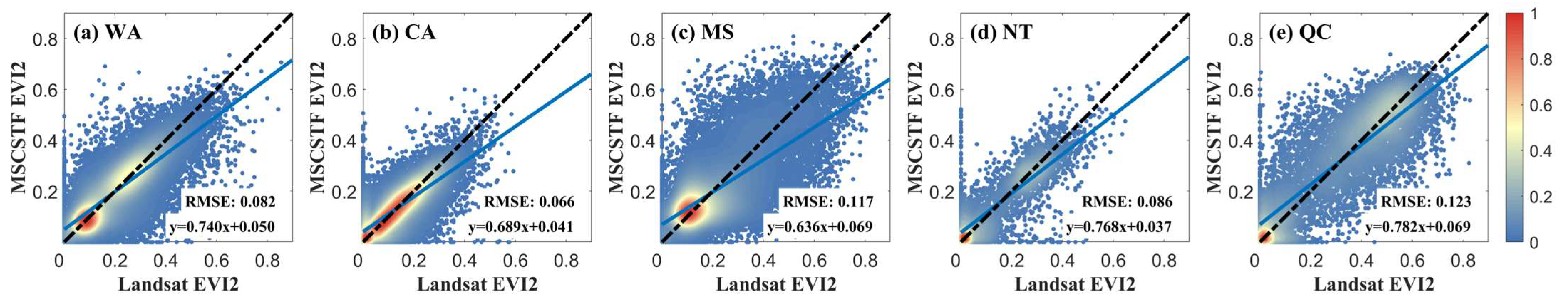
Figure 6 shows scatter density plots between all available cloud-free resampled Landsat data prior to 2000 and the corresponding MSCSTF results in the five regions. The scatter distribution map illustrates that the overall reconstructed MSCSTF results have relatively clustered scatter distributions, small errors, and high linear fitting degrees when compared to the Landsat data. In WA and CA, the error between the MSCSTF results and the validation data is small, with an RMSE of 0.082 and 0.066, respectively, thus indicating robust agreement. In addition, the fitness between them is high, particularly within the EVI2 values below 0.3, exhibiting a dense clustering along the 1:1 line. Note that the results typically present underestimations, with specific underestimations at high values and overestimations at low values, as revealed by the regression slopes of 0.740, 0.689, 0.636, 0.768, and 0.782, along with positive regression intercepts in the respective regions.

4.2. Comparisons of Fused Results with MODIS and Landsat Data after 2000

Figure 7 displays the spatial distributions of the MODIS, Landsat, and fused MODIS-like data at two dates after 2000 in the five regions. The spatial distribution map illustrates that the fused MODIS-like data are consistent with the MODIS data in terms of both spatial details and spatial distribution, while they present underestimations compared to the Landsat data. The fused results present considerable moderate-resolution-grained details with the MODIS data. As shown in Figure 8, the fused results have low biases and high linear correlations with the MODIS data, as demonstrated by the low RMSE and high regression slopes, respectively. Compared with the Landsat data, the fused results have certain underestimations, as indicated by the regression slopes of 0.595, 0.610, 0.503, 0.690, and 0.843 in the five regions. The situations of scatter clustering distribution and underestimation are similar to those observed in the retrospective reconstruction experiments, demonstrating that the modeled retrospective MODIS-like data can reflect actual moderate-resolution land surface situations to some extent.

As found in this study, the modeled MODIS-like results in MS are relatively worse than those in other areas, which is primarily due to the complexity presented in MS. The MS region, situated along the Mississippi River, is predominantly characterized by croplands. The land surface reflectance of these croplands is significantly influenced by the variety of crop types and phenological stages, leading to a pronounced surface spatial heterogeneity and obvious seasonal variations. This intricate landscape poses a substantial challenge for spatiotemporal fusion techniques.

4.3. Comparisons of Spatiotemporal Fusion Models

To demonstrate the effectiveness of MSCSTF and other models in simulating MODIS-like data, Figure 9 compares the spatial distributions of the results modeled using MSCSTF and six other spatiotemporal fusion models, including three deep-learning-based models (i.e., EDCSTFN, StfNet, and BiaSTF) and three traditional rule-based models (i.e., FSDAF2, cuFSDAF, and RASDF), across the five regions. The results obtained by MSCSTF are consistent with the MODIS data in terms of spatial distribution and are more closely aligned with the MODIS acquisitions than those modeled by other models, especially in the MS, NT, and QC regions. StfNet and EDCSTFN perform well in CA, but they perform worse in MS and NT. The fused results obtained by using BiaSTF, FSDAF2, cuFSDAF, and RASDF exhibit significant differences in all of the regions and deviate from the MODIS observations visually. These inconsistencies arise primarily because they simulate the target MODIS-like data by directly adding temporal changes that have been generated via spatiotemporal fusion to the reference high-resolution data, which, in this case, are the resampled Landsat data. The systematic biases between the MODIS and Landsat data have not been mitigated and are incorporated into the fused results simulated by these four models.

Based on the synthetic analysis using scatter density plots (Figure 10) and the quantitative assessment (

Table 5. Quantitative evaluation of different spatiotemporal fusion models. The bold data denote the best evaluation metrics. The regional average AD is the mean of each absolute AD values obtained from the five regions.

Metrics	Models	WA	CA	MS	NT	QC	Average
RMSE	MSCSTF	0.038	0.029	0.111	0.051	0.058	0.058
	EDCSTFN	0.039	0.029	0.115	0.067	0.064	0.063
	StfNet	0.041	0.029	0.117	0.067	0.070	0.065
	BiaSTF	0.106	0.076	0.195	0.120	0.157	0.131
	FSDAF2	0.106	0.068	0.192	0.103	0.131	0.120
	cuFSDAF	0.103	0.064	0.187	0.107	0.179	0.128
	RASDF	0.105	0.070	0.201	0.088	0.127	0.118
SSIM	MSCSTF	0.820	0.841	0.387	0.719	0.605	0.674
	EDCSTFN	0.800	0.862	0.320	0.620	0.585	0.637
	StfNet	0.773	0.834	0.373	0.678	0.525	0.636
	BiaSTF	0.311	0.383	0.181	0.293	0.224	0.278
	FSDAF2	0.390	0.478	0.171	0.347	0.253	0.328
	cuFSDAF	0.400	0.494	0.175	0.319	0.174	0.312
	RASDF	0.390	0.469	0.164	0.396	0.265	0.337
R	MSCSTF	0.943	0.944	0.631	0.917	0.889	0.865
	EDCSTFN	0.939	0.950	0.583	0.856	0.863	0.838
	StfNet	0.934	0.946	0.639	0.889	0.835	0.849
	BiaSTF	0.768	0.739	0.378	0.639	0.519	0.609
	FSDAF2	0.814	0.828	0.398	0.734	0.629	0.681
	cuFSDAF	0.822	0.839	0.394	0.718	0.520	0.659
	RASDF	0.819	0.818	0.378	0.754	0.627	0.679
AD	MSCSTF	0.017	0.011	−0.026	−0.032	0.011	0.019
	EDCSTFN	0.022	0.014	−0.042	−0.045	0.013	0.027
	StfNet	0.017	0.009	−0.064	−0.059	0.011	0.032
	BiaSTF	0.020	−0.031	−0.072	−0.004	−0.023	0.030
	FSDAF2	0.048	0.032	−0.045	−0.023	0.011	0.032
	cuFSDAF	0.049	0.031	−0.050	−0.030	0.009	0.034
	RASDF	0.048	0.032	−0.049	−0.028	0.013	0.034

), we found that the MSCSTF results exhibit small errors, high similarities, and high correlations with the MODIS data. MSCSTF is superior to the other models, with a regional average RMSE, SSIM, R, and an absolute AD of 0.058, 0.674, 0.865, and 0.019, respectively. Compared to the other spatiotemporal fusion models, MSCSTF exhibits strong performance in WA, NT, and QC, as evidenced by the low RMSE values (0.038, 0.051, and 0.058, respectively), high SSIM values (0.820, 0.719, and 0.605, respectively), and high R values (0.943, 0.917, and 0.889, respectively). In CA, MSCSTF, StfNet, and EDCSTFN display a comparable performance, with an RMSE of 0.029. BiaSTF, FSDAF2, cuFSDAF, and RASDF show lower accuracies, as indicated by an average RMSE of 0.131, 0.120, 0.128, and 0.118, respectively, and exhibit a low correlation, with an average R of 0.609, 0.681, 0.659, and 0.679, respectively.

4.4. Modular Ablation

Figure 11 and

Table 6. The same as Figure 5, but for comparisons with modular ablation. The bold data denote the best evaluation metrics.

Metrics	Models	WA	CA	MS	NT	QC	Average
RMSE	MSCSTF	0.038	0.029	0.111	0.051	0.058	0.057
	MSCSTF w/o multi-scale	0.040	0.035	0.118	0.060	0.069	0.065
	MSCSTF w/o Landsat-correction	0.039	0.030	0.115	0.055	0.058	0.059
	MSCSTF w/o AVHRR-correction	0.040	0.034	0.110	0.052	0.061	0.059
SSIM	MSCSTF	0.820	0.841	0.387	0.719	0.605	0.674
	MSCSTF w/o multi-scale	0.792	0.817	0.370	0.691	0.500	0.634
	MSCSTF w/o Landsat-correction	0.810	0.832	0.378	0.710	0.613	0.669
	MSCSTF w/o AVHRR-correction	0.811	0.799	0.378	0.719	0.629	0.667
R	MSCSTF	0.943	0.944	0.631	0.917	0.889	0.865
	MSCSTF w/o multi-scale	0.940	0.915	0.617	0.897	0.832	0.840
	MSCSTF w/o Landsat-correction	0.943	0.945	0.631	0.907	0.892	0.864
	MSCSTF w/o AVHRR-correction	0.942	0.933	0.638	0.915	0.894	0.864
AD	MSCSTF	0.017	0.011	−0.026	−0.032	0.011	0.019
	MSCSTF w/o multi-scale	0.021	0.003	−0.055	−0.045	−0.004	0.026
	MSCSTF w/o Landsat-correction	0.014	0.016	−0.049	−0.038	0.021	0.027
	MSCSTF w/o AVHRR-correction	0.015	0.018	−0.035	−0.033	0.033	0.027

reveal that the MSCSTF results are more consistent with the MODIS data in most regions when compared to the results of other models, with the lowest RMSE values of 0.038, 0.029, 0.051, and 0.058 in WA, CA, NT, and QC, respectively, while MSCSTF w/o AVHRR-correction performs slightly better in MS, with an RMSE of 0.110. MSCSTF w/o multi-scale shows the worst performances in most regions, as evidenced by the assessment metrics, thus demonstrating that the multi-scale module used to address the spatial-scale issues is effective in avoiding introducing unrealistic errors and enhancing the robustness of the fusion models. The models without Landsat or AVHRR-correction perform comparably, illustrating that bias mitigations of AVHRR and Landsat data are of importance. In conclusion, the introductions of multi-scale and image correction modules are essential to resolve the spatial-scale gap and systematic biases among the images acquired from three distinct sensors and to achieve a robust model for generating MODIS-like data.

5. Discussion

The biggest difference in MSCSTF when compared to existing spatiotemporal fusion models lies in the reference high-resolution Landsat data input and the target MODIS data, which are acquired by different sensors, thus leading to differences in spatial resolution and quality. The generation of MODIS-like data can also be conducted by blending AVHRR and MODIS image pairs, and MODIS images at the reference time are required. In this way, a method for reconstructing pre-2000 MODIS-like data is to take MODIS images after 2000 as high-resolution inputs at the reference time. However, long time intervals between the reference and target time may not guarantee the attainment of inter-annual variations in fused moderate-resolution data. Landsat data have been available since 1972 and provide much finer spatial details than MODIS images, making them suitable fine-spatial-resolution inputs for reconstructing MODIS-like data. Thus, the proposed scheme that blends AVHRR and Landsat images to reconstruct MODIS-like data is reasonable.

The performance of MSCSTF surpasses that of comparative spatiotemporal fusion models in this study, mainly because the comparative models were not designed to address the issues arising from the substantial differences in spatial scale between the inputs and the inherent systematic biases among the images obtained from three different sensors. Errors may be introduced if the biases between the Landsat and AVHRR data and the MODIS data are not eliminated before fusion. Additionally, the inaccuracies observed in the results of BiaSTF, FSDAF2, cuFSDAF, and RASDF are primarily attributed to the fact that they create MODIS-like data by simulating temporal changes between the reference and target times, and by adding the modeled changes to the reference Landsat image, rather than the reference MODIS images.

While MSCSTF demonstrates superior simulation performance compared to the rule-based models in this study, it is imperative to critically acknowledge the strengths of rule-based models. Advanced rule-based spatiotemporal fusion models commonly integrate mixed pixel decomposition, spatial interpolation, and distributed residuals to accurately simulate fine-grained temporal changes, which are supported by a robust physical foundation that enhances our comprehension of spatiotemporal patterns. Notably, rule-based models do not require extensive training data, while deep learning models rely heavily on high-quality training data. Furthermore, deep learning models demand substantial computational resources during training, thereby presenting challenges in terms of hardware and time constraints for executing large-scale experiments.

In some results, the modeled MODIS-like data appear slightly blurrier than the MODIS data. However, the MODIS-like data can still reasonably capture spatial details at 500-m resolution, similar to MODIS data. Spatiotemporal fusion models typically operate in two types of simulation. The first involves simulating temporal changes and then adding these changes into the high-resolution images captured at the reference time to derive fusion outcomes. The second way entails directly integrating the input images to simulate fusion results. The former method excels in preserving spatial details within high-resolution images, whereas the latter often results in blurriness. In our study, significant differences exist between the reference high-resolution Landsat images and the target MODIS data. Consequently, uncertainty may arise in employing the first method, prompting us to resort to the second method, thus leading to the blurriness issue. Some scholars have tested models based on generative adversarial networks and have found that they have the potential to overcome the blurriness issue caused by convolutional neural networks, warranting further exploration in the future.

One point that cannot be ignored is that using resampled Landsat data as validation data to assess the accuracy of MODIS-like data before 2000 may not be accurate, as Landsat 5 TM sensor and MODIS sensor differ in wavelengths and imaging quality, resulting in some discrepancies between the resampled Landsat images and the actual MODIS images. While common linear or nonlinear mapping methods (such as linear transformation, random forests, and support vector regression) can be utilized to calibrate the resampled Landsat data and fit them to the MODIS data, there remains significant uncertainties. Using these uncertain Landsat data as the ground truth could further impact the conclusions of the research. Therefore, we directly used the Landsat images that were resampled using the moving average method as the validation data.

In addition to retrospective reconstruction, it is worth considering the generation of future MODIS-like data after the retirement of MODIS sensors. The MODIS sensors have already far exceeded their design lifespan of six years, and they may not provide high-quality data in the near future. The latest Landsat 9 and Metop-C satellites were launched in September 2021 and November 2018, respectively, and, although their design lifetimes are both five years, it is highly possible that their actual service periods will surpass a decade. The proposed model seems to offer a reliable solution for producing future MODIS-like data by blending Landsat and AVHRR images. Of course, the differences in sensor generations present great challenges, and there is still much room for improvement during modeling.

6. Conclusions

MODIS products with moderate spatial resolution and frequent temporal coverage are favorable to use in large-scale land surface studies. The lack of MODIS data prior to 2000 hinders the retrospective simulations and analyses that use moderate-spatial-resolution data. Herein, we have presented a multi-scale spatiotemporal fusion model based on a convolutional neural network to generate MODIS-like data by combining Landsat and AVHRR data. The model blends AVHRR and Landsat images using a multi-scale feature extraction module, aiming to address the large spatial resolution difference between them. An image correction module was incorporated into the network using deep supervision to mitigate the synthetic deviations between the AVHRR and Landsat images and the MODIS data. The fused MODIS-like results show comparable spatial distributions with the observed MODIS data when comparing the results with the MODIS data in five study regions. The proposed model displays good performance in reconstructing retrospective MODIS-like data. Compared to six existing data fusion models, the developed model presented a robust performance in terms of spatiotemporal distributions. The proposed model attained regional average quantitative indicators of 0.058, 0.674, 0.865, and 0.019 for RMSE, SSIM, R, and AD, respectively, and surpassed the six comparative models in most regions. The proposed MSCSTF avoids using MODIS data during the prediction phase and possesses the capability to reconstruct spatiotemporal continuous MODIS-like data prior to 2000 to facilitate retrospective research.

References

- Vinnikov, K.Y.; Grody, N.C. Global Warming Trend of Mean Tropospheric Temperature Observed by Satellites. Science 2003, 302, 269–272. [Google Scholar] [CrossRef] [PubMed]
- Prabhakara, C.; Iacovazzi, J.R.; Yoo, J.M.; Dalu, G. Global warming: Evidence from satellite observations. Geophys. Res. Lett. 2000, 27, 3517–3520. [Google Scholar] [CrossRef]
- Overpeck, J.T.; Meehl, G.A.; Bony, S.; Easterling, D.R. Climate Data Challenges in the 21st Century. Science 2011, 331, 700–702. [Google Scholar] [CrossRef] [PubMed]
- Yang, J.; Gong, P.; Fu, R.; Zhang, M.; Chen, J.; Liang, S.; Xu, B.; Shi, J.; Dickinson, R. The role of satellite remote sensing in climate change studies. Nat. Clim. Chang. 2013, 3, 875–883. [Google Scholar] [CrossRef]
- Reichstein, M.; Camps-Valls, G.; Stevens, B.; Jung, M.; Denzler, J.; Carvalhais, N.; Prabhat, F. Deep learning and process understanding for data-driven Earth system science. Nature 2019, 566, 195–204. [Google Scholar] [CrossRef] [PubMed]
- Park, T.; Ganguly, S.; Tømmervik, H.; Euskirchen, E.S.; Høgda, K.A.; Karlsen, S.R.; Brovkin, V.; Nemani, R.R.; Myneni, R.B. Changes in growing season duration and productivity of northern vegetation inferred from long-term remote sensing data. Environ. Res. Lett. 2016, 11, 084001. [Google Scholar] [CrossRef]
- Wild, B.; Teubner, I.; Moesinger, L.; Zotta, R.M.; Forkel, M.; Van der Schalie, R.; Sitch, S.; Dorigo, W. VODCA2GPP—A new, global, long-term (1988–2020) gross primary production dataset from microwave remote sensing. Earth Syst. Sci. Data 2022, 14, 1063–1085. [Google Scholar] [CrossRef]
- Chen, J.; Ju, W.; Ciais, P.; Viovy, N.; Liu, R.; Liu, Y.; Lu, X. Vegetation structural change since 1981 significantly enhanced the terrestrial carbon sink. Nat. Commun. 2019, 10, 4259. [Google Scholar] [CrossRef]
- Wang, K.; Dickinson, R.E. A review of global terrestrial evapotranspiration: Observation, modeling, climatology, and climatic variability. Rev. Geophys. 2012, 50, RG2005. [Google Scholar] [CrossRef]
- Healey, S.P.; Cohen, W.B.; Zhiqiang, Y.; Krankina, O.N. Comparison of Tasseled Cap-based Landsat data structures for use in forest disturbance detection. Remote Sens. Environ. 2005, 97, 301–310. [Google Scholar] [CrossRef]
- Masek, J.G.; Huang, C.; Wolfe, R.; Cohen, W.; Hall, F.; Kutler, J.; Nelson, P. North American forest disturbance mapped from a decadal Landsat record. Remote Sens. Environ. 2008, 112, 2914–2926. [Google Scholar] [CrossRef]
- White, J.C.; Wulder, M.A.; Hermosilla, T.; Coops, N.C.; Hobart, G.W. A nationwide annual characterization of 25 years of forest disturbance and recovery for Canada using Landsat time series. Remote Sens. Environ. 2017, 194, 303–321. [Google Scholar] [CrossRef]
- Tucker, C.J.; Pinzon, J.E.; Brown, M.E.; Slayback, D.A.; Pak, E.W.; Mahoney, R.; Vermote, E.F.; El Saleous, N. An extended AVHRR 8-km NDVI dataset compatible with MODIS and SPOT vegetation NDVI data. Int. J. Remote Sens. 2005, 26, 4485–4498. [Google Scholar] [CrossRef]
- Wu, W.; Sun, Y.; Xiao, K.; Xin, Q. Development of a global annual land surface phenology dataset for 1982–2018 from the AVHRR data by implementing multiple phenology retrieving methods. Int. J. Appl. Earth Obs. Geoinf. 2021, 103, 102487. [Google Scholar] [CrossRef]
- Liu, Y.; Liu, R.; Chen, J. Retrospective retrieval of long-term consistent global leaf area index (1981–2011) from combined AVHRR and MODIS data. J. Geophys. Res. Biogeosci. 2012, 117, G04003. [Google Scholar] [CrossRef]
- Fensholt, R.; Proud, S.R. Evaluation of Earth Observation based global long term vegetation trends—Comparing GIMMS and MODIS global NDVI time series. Remote Sens. Environ. 2012, 119, 131–147. [Google Scholar] [CrossRef]
- Mu, Q.; Zhao, M.; Kimball, J.S.; McDowell, N.G.; Running, S.W. A Remotely Sensed Global Terrestrial Drought Severity Index. Bull. Am. Meteorol. Soc. 2013, 94, 83–98. [Google Scholar] [CrossRef]
- Justice, C.O.; Vermote, E.; Townshend, J.R.; Defries, R.; Roy, D.P.; Hall, D.K.; Salomonson, V.V.; Privette, J.L.; Riggs, G.; Strahler, A.; et al. The Moderate Resolution Imaging Spectroradiometer (MODIS): Land remote sensing for global change research. IEEE Trans. Geosci. Remote. Sens. 1998, 36, 1228–1249. [Google Scholar] [CrossRef]
- Friedl, M.A.; Sulla-Menashe, D.; Tan, B.; Schneider, A.; Ramankutty, N.; Sibley, A.; Huang, X. MODIS Collection 5 global land cover: Algorithm refinements and characterization of new datasets. Remote Sens. Environ. 2010, 114, 168–182. [Google Scholar] [CrossRef]
- Yin, H.; Pflugmacher, D.; Kennedy, R.E.; Sulla-Menashe, D.; Hostert, P. Mapping Annual Land Use and Land Cover Changes Using MODIS Time Series. IEEE J. Sel. Top. Appl. Earth Obs. Remote Sens. 2014, 7, 3421–3427. [Google Scholar] [CrossRef]
- Piao, S.; Huang, M.; Liu, Z.; Wang, X.; Ciais, P.; Canadell, J.G.; Wang, K.; Bastos, A.; Friedlingstein, P.; Houghton, R.A.; et al. Lower land-use emissions responsible for increased net land carbon sink during the slow warming period. Nat. Geosci. 2018, 11, 739–743. [Google Scholar] [CrossRef]
- Chen, M.; Zhuang, Q.; Cook, D.R.; Coulter, R.; Pekour, M.; Scott, R.L.; Munger, J.W.; Bible, K. Quantification of terrestrial ecosystem carbon dynamics in the conterminous United States combining a process-based biogeochemical model and MODIS and AmeriFlux data. Biogeosciences 2011, 8, 2665–2688. [Google Scholar] [CrossRef]
- Zhu, X.; Cai, F.; Tian, J.; Williams, T.K. Spatiotemporal Fusion of Multisource Remote Sensing Data: Literature Survey, Taxonomy, Principles, Applications, and Future Directions. Remote Sens. 2018, 10, 527. [Google Scholar] [CrossRef]
- Shi, W.Z.; Guo, D.Z.; Zhang, H. A reliable and adaptive spatiotemporal data fusion method for blending multi-spatiotemporal-resolution satellite images. Remote Sens. Environ. 2022, 268, 112770. [Google Scholar] [CrossRef]
- Gao, F.; Masek, J.; Schwaller, M.; Hall, F. On the blending of the Landsat and MODIS surface reflectance: Predicting daily Landsat surface reflectance. IEEE Trans. Geosci. Remote. Sens. 2006, 44, 2207–2218. [Google Scholar]
- Zhu, X.; Chen, J.; Gao, F.; Chen, X.; Masek, J.G. An enhanced spatial and temporal adaptive reflectance fusion model for complex heterogeneous regions. Remote Sens. Environ. 2010, 114, 2610–2623. [Google Scholar] [CrossRef]
- Emelyanova, I.V.; McVicar, T.R.; Van Niel, T.G.; Li, L.T.; Van Dijk, A.I.J.M. Assessing the accuracy of blending Landsat–MODIS surface reflectances in two landscapes with contrasting spatial and temporal dynamics: A framework for algorithm selection. Remote Sens. Environ. 2013, 133, 193–209. [Google Scholar] [CrossRef]
- Zhu, X.; Helmer, E.H.; Gao, F.; Liu, D.; Chen, J.; Lefsky, M.A. A flexible spatiotemporal method for fusing satellite images with different resolutions. Remote Sens. Environ. 2016, 172, 165–177. [Google Scholar] [CrossRef]
- Wang, Q.; Atkinson, P.M. Spatio-temporal fusion for daily Sentinel-2 images. Remote Sens. Environ. 2018, 204, 31–42. [Google Scholar] [CrossRef]
- Zhao, Y.; Huang, B.; Song, H. A robust adaptive spatial and temporal image fusion model for complex land surface changes. Remote Sens. Environ. 2018, 208, 42–62. [Google Scholar] [CrossRef]
- Liu, M.; Yang, W.; Zhu, X.; Chen, J.; Chen, X.; Yang, L.; Helmer, E.H. An Improved Flexible Spatiotemporal DAta Fusion (IFSDAF) method for producing high spatiotemporal resolution normalized difference vegetation index time series. Remote Sens. Environ. 2019, 227, 74–89. [Google Scholar] [CrossRef]
- Liu, S.; Zhou, J.; Qiu, Y.; Chen, J.; Zhu, X.; Chen, H. The FIRST model: Spatiotemporal fusion incorrporting spectral autocorrelation. Remote Sens. Environ. 2022, 279, 113111. [Google Scholar] [CrossRef]
- Li, J.; Li, Y.; Cai, R.; He, L.; Chen, J.; Plaza, A. Enhanced Spatiotemporal Fusion via MODIS-Like Images. IEEE Trans. Geosci. Remote Sens. 2022, 60, 5610517. [Google Scholar] [CrossRef]
- Qiu, Y.; Zhou, J.; Chen, J.; Chen, X. Spatiotemporal fusion method to simultaneously generate full-length normalized difference vegetation index time series (SSFIT). Int. J. Appl. Earth Obs. Geoinf. 2021, 100, 102333. [Google Scholar] [CrossRef]
- Tan, Z.; Yue, P.; Di, L.; Tang, J. Deriving High Spatiotemporal Remote Sensing Images Using Deep Convolutional Network. Remote Sens. 2018, 10, 1066. [Google Scholar] [CrossRef]
- Tan, Z.; Di, L.; Zhang, M.; Guo, L.; Gao, M. An Enhanced Deep Convolutional Model for Spatiotemporal Image Fusion. Remote Sens. 2019, 11, 2898. [Google Scholar] [CrossRef]
- Liu, X.; Deng, C.; Chanussot, J.; Hong, D.; Zhao, B. StfNet: A Two-Stream Convolutional Neural Network for Spatiotemporal Image Fusion. IEEE Trans. Geosci. Remote Sens. 2019, 57, 6552–6564. [Google Scholar] [CrossRef]
- Li, W.; Zhang, X.; Peng, Y.; Dong, M. DMNet: A Network Architecture Using Dilated Convolution and Multiscale Mechanisms for Spatiotemporal Fusion of Remote Sensing Images. IEEE Sens. J. 2020, 20, 12190–12202. [Google Scholar] [CrossRef]
- Li, W.; Zhang, X.; Peng, Y.; Dong, M. Spatiotemporal Fusion of Remote Sensing Images using a Convolutional Neural Network with Attention and Multiscale Mechanisms. Int. J. Remote Sens. 2021, 42, 1973–1993. [Google Scholar] [CrossRef]
- Song, H.; Liu, Q.; Wang, G.; Hang, R.; Huang, B. Spatiotemporal Satellite Image Fusion Using Deep Convolutional Neural Networks. IEEE J. Sel. Top. Appl. Earth Obs. Remote Sens. 2018, 11, 821–829. [Google Scholar] [CrossRef]
- Yuan, Q.; Wei, Y.; Meng, X.; Shen, H.; Zhang, L. A Multiscale and Multidepth Convolutional Neural Network for Remote Sensing Imagery Pan-Sharpening. IEEE J. Sel. Top. Appl. Earth Obs. Remote Sens. 2018, 11, 978–989. [Google Scholar] [CrossRef]
- Chen, Y.; Shi, K.; Ge, Y.; Zhou, Y. Spatiotemporal Remote Sensing Image Fusion Using Multiscale Two-Stream Convolutional Neural Networks. IEEE Trans. Geosci. Remote Sens. 2022, 60, 4402112. [Google Scholar] [CrossRef]
- Wang, Q.; Zhang, Y.; Onojeghuo, A.O.; Zhu, X.; Atkinson, P.M. Enhancing Spatio-Temporal Fusion of MODIS and Landsat Data by Incorporating 250 m MODIS Data. IEEE J. Sel. Top. Appl. Earth Obs. Remote Sens. 2017, 10, 4116–4123. [Google Scholar] [CrossRef]
- Shao, Z.; Cai, J.; Fu, P.; Hu, L.; Liu, T. Deep learning-based fusion of Landsat-8 and Sentinel-2 images for a harmonized surface reflectance product. Remote Sens. Environ. 2019, 235, 111425. [Google Scholar] [CrossRef]
- Sdraka, M.; Papoutsis, I.; Psomas, B.; Vlachos, K.; Ioannidis, K.; Karantzalos, K.; Gialampoukidis, I.; Vrochidis, S. Deep Learning for Downscaling Remote Sensing Images: Fusion and super-resolution. IEEE Geosc. Rem. Sens. M. 2022, 10, 202–255. [Google Scholar] [CrossRef]
- Ao, Z.; Sun, Y.; Pan, X.; Xin, Q. Deep Learning-Based Spatiotemporal Data Fusion Using a Patch-to-Pixel Mapping Strategy and Model Comparisons. IEEE Trans. Geosci. Remote Sens. 2022, 60, 5407718. [Google Scholar] [CrossRef]
- Jiang, Z.; Huete, A.R.; Didan, K.; Miura, T. Development of a two-band enhanced vegetation index without a blue band. Remote Sens. Environ. 2008, 112, 3833–3845. [Google Scholar] [CrossRef]
- Li, D.; Chen, Q. Dynamic hierarchical mimicking towards consistent optimization objectives. In Proceedings of the IEEE/CVF Conference on Computer Vision and Pattern Recognition (CVPR), Seattle, WA, USA, 14–19 June 2020; pp. 7642–7651. [Google Scholar]
- Lee, C.Y.; Xie, S.; Gallagher, P.; Zhang, Z.; Tu, Z. Deeply-Supervised Nets. In Proceedings of the Eighteenth International Conference on Artificial Intelligence and Statistics, PMLR, San Diego, CA, USA, 9–12 May 2015; Volume 38, pp. 562–570. [Google Scholar]
- Wang, Z.; Simoncelli, E.P.; Bovik, A.C. Multiscale structural similarity for image quality assessment. In Proceedings of the Thirty-Seventh Asilomar Conference on Signals, Systems & Computers, Pacific Grove, CA, USA, 9–12 November 2003; Volume 1392, pp. 1398–1402. [Google Scholar]
- Lai, W.S.; Huang, J.B.; Ahuja, N.; Yang, M.H. Deep laplacian pyramid networks for fast and accurate super-resolution. In Proceedings of the IEEE Conference on Computer Vision and Pattern Recognition (CVPR), Honolulu, HI, USA, 21–26 July 2017; pp. 624–632. [Google Scholar]
- Guo, D.; Shi, W.; Hao, M.; Zhu, X. FSDAF 2.0: Improving the performance of retrieving land cover changes and preserving spatial details. Remote Sens. Environ. 2020, 248, 111973. [Google Scholar] [CrossRef]
- Gao, H.; Zhu, X.; Guan, Q.; Yang, X.; Yao, Y.; Zeng, W.; Peng, X. cuFSDAF: An Enhanced Flexible Spatiotemporal Data Fusion Algorithm Parallelized Using Graphics Processing Units. IEEE Trans. Geosci. Remote. Sens. 2022, 60, 4403016. [Google Scholar] [CrossRef]
Figure 1.
Locations and land cover distributions of the study regions, including areas in WA, CA, MS, NT, and QC, respectively. The base map is the land cover distribution product based on the University of Maryland land cover classification across North America. The enlarged sub-map displays the land cover in each region.
Figure 2.
An illustrative scheme for the structure of the proposed MSCSTF.
Figure 3.
Schematic diagrams of nonlinear spatial pyramid mapping constructed by integrating upscaling and downscaling.
Figure 4.
Schematic diagrams of traditional deep supervisions in a traditional form and in MSCSTF.
Figure 5.
Spatial distributions of Landsat and fused MODIS-like data in five regions at two dates prior to 2000. As shown at subfigures (a–t), columns 1 and 3 refer the resampled Landsat images at two dates, and columns 2 and 4 represent the MSCSTF results at the corresponding dates. Rows 1–5 represent data in WA, CA, MS, NT, and QC, respectively.
Figure 6.
Scatter density plots between all available cloud-free Landsat data prior to 2000 and modeled MODIS-like data at corresponding dates for the study areas of WA, CA, MS, NT, and QC, respectively. The dotted and blue lines denote the 1:1 line and linear regression line. The color bar at the right-hand side refers to the relative scatter density.
Figure 7.
The same as
Figure 5, but for spatial distributions of MODIS, Landsat data, and the modeled MODIS-like data after 2000. The subplots (
a–
c) correspond to the results of MODIS, Landsat, and MSCSTF in WA on 30 September 2014. Subplots (
d–
f) correspond to WA on 16 October 2018. Subplots (
g–
i) correspond to CA on 29 August 2014. Subplots (
j–
l) correspond to CA on 6 September 2018. Subplots (
m–
o) correspond to MS on 8 May 2016. Subplots (
p–
r) correspond to MS on 16 October 2017. Subplots (
s–
u) correspond to NT on 29 August 2013. Subplots (
v–
x) correspond to NT on 15 April 2014. Subplots (
y–
aa) correspond to QC on 26 February 2001. Subplots (
ab–
ad) correspond to QC on 14 September 2009.
Figure 8.
Figure 6, but for comparisons between modeled MODIS-like data and MODIS data (subplots (
e)), and between modeled MODIS-like data and Landsat data (subplots (
f–
j)) at dates corresponding to the above spatial distribution map. The dotted and blue lines denote the 1:1 line and linear regression line.
Figure 9.
Spatial distributions of results fused by different spatiotemporal fusion models in five regions after 2000. Columns 1–8 represent spatial distributions of results obtained by MODIS, MSCSTF, EDCSTFN, StfNet, BiaSTF, FSDAF2, cuFSDAF, and RASDF, respectively. Rows 1–5 (subplots (a–h), subplots (i–p), subplots (q–x), subplot (y–af), and subplot (ag–an)) represent the results in WA, CA, MS, NT, and QC, respectively.
Figure 10.
Scatter density plots of results fused by different spatiotemporal fusion models. Columns 1–7 represent scatter density comparisons between results modeled by MSCSTF, EDCSTFN, StfNet, BiaSTF, FSDAF2, cuFSDAF, and RASDF with MODIS data, respectively. Rows 1–5 (subplots (a–g), subplots (h–n), subplots (o–u), subplot (v–ab), and subplot (ac–ai)) represent the results in WA, CA, MS, NT, and QC, respectively.
Figure 11.
Figure 9, but for comparisons with modular ablation. Rows 1–5 (subplots (
e), subplots (
j), subplots (
k–
o), subplot (
t), and subplot (
u–
y)) represent the results in WA, CA, MS, NT, and QC, respectively.