Monitoring Thermal Exchange of Hot Water Mass via Underwater Acoustic Tomography with Inversion and Optimization Method

Abstract

Thermal exchange of underwater water mass caused by marine heat wave is a hot point of research recently. In particular, because the water temperature observation along hot water mass transportation is hard work. Acoustic tomography is an advanced method to measure water temperature variations via sound signal transmission with multi-station network sensing. The 5 kHz frequency acoustic tomography used for observing water temperature variations caused by ocean heat waves is interesting work. In this paper, the numerical simulation of hot water mass is completed first, then floatation and diffusion of hot water mass in a simulation are monitored by acoustic tomography. A new inversion optimization method is proposed to obtain hot water mass transportation variations at two-dimensional temperature vertical profile. The proposed inversion method adds a regularized mode matrix and the optimization method adds the model correlation matrix to improve the results quality. The accuracy of inversion optimization results is compared and discussed, where the mean temperature error is less than 0.4 °C. Sensing water temperature variation of marine heat waves is verified via acoustic signal transmission and improved inversion optimization method. The water dynamical process observation is an application of acoustic tomography, which can be further used observe underwater environmental characteristics.

1. Introduction

Marine heat waves have gradually become an important observation in ocean environmental research. The concept of the ‘marine heat wave’ was introduced by Pearce et al. [1], who describe this ocean climate phenomenon as: an unusually warm seawater incident that exerts sustained impacts on marine systems. In the ocean, such climate phenomena often trend to water temperature anomalies. The horizontal scales of water temperature anomalies are normally up to several kilometers, the vertical scales are extending from the sea surface to bottom at depths of hundreds of meters, and time scales ranging from days to years [2,3,4].

The marine heat wave variations are directly related to sea surface temperature (SST), water heat exchange at air-sea interface and multi-scale ocean dynamical processes (like water mass transportation and mixing). SST variations and water heat exchange can be effectively measured by satellite or surface observation. However, underwater multi-scale dynamical processes also play an important role in the marine heat wave progress. For example, when the upwelling is weakened or the downwelling is strengthened, warm water accumulation promotes the occurrence of marine heat waves [5]. Conversely, it slows the intensity of marine heat waves when the upwelling is strengthened or downwelling is weakened [6]. In coastal regions, upwelling fluctuations largely influence the marine heat wave seasonal characteristics. Researchers found that marine heat waves mainly exist during the weakening periods of coastal upwelling (fall and winter) in the west coast of the United States, where the intensity of marine heat wave increases to 2 °C [7]. On the other hand, in the Northeast Pacific, hot water mass transporting and mixing have significant influence on the evolution of marine heat waves [8,9,10]. Water transportation brings warmer (cooler) seawater from the subsurface layer to the mixing layer, which enhances (weakens) the intensity of marine heat wave. As such, the intensity of marine heat waves under the influence of high pressure can increase 2.1~3.1 °C in winter [9].

Thus, the underwater heat exchange in multi-scale ocean dynamical processes is a problem worthy of attention and further study. However, water transportation with heat exchange in vertical profile scale still lack refined observation methods. For this reason, we try to use underwater acoustic tomography technology as an advanced observation method for monitoring the water transportation process.

In underwater acoustic tomography study, ocean acoustic tomography (OAT) is firstly proposed by Munk and Wunsch for estimating the ocean temperature or current velocity over a wide area [11]. The key to acoustic tomography is to establish the functional relationship between an underwater environment and the acoustic signal, where the marine physical parameters (temperature, salinity and velocity) are obtained by the variation of acoustic signal travel time [12,13,14]. With the development of advanced technology, acoustic tomography observation is used more frequently in coastal area via high frequency signal transmission as coastal acoustic tomography (CAT). Several high-precision experiments have verified the feasibility for the observation of ocean dynamic processes via CAT [15,16,17,18]. We previously have successfully obtained signal transmission within a spatial area and reconstructed the three-dimensional flow current and water temperature field via moving acoustic tomography in preliminary experiments [17]. Chen et al. reconstructed two-dimensional flow fields using a coast-fitting inversion model by five-station reciprocal transmission and obtained the M2 and M4 tidal currents and residual current [18].

Thus, whether water transportation with heat exchange can be observed and estimated by acoustic tomography is discussed in this paper. Here, we call this process hot water mass transportation. To simplify the simulation model, hot water transportation mainly contains the flotation and diffusion of hot water mass. The simulation model is established and compared with acoustic tomography results. An inversion optimization method, using a regularized mode matrix and model correlation matrix, is proposed to reconstruct the water temperature variations via the signal travel time differences. In addition, water mass transportation route is obtained by judging the temperature sensitive position. The inversion results are compared to discuss the possibility of monitoring the flotation and diffusion in hot water mass transportation.

The remaining sections of this paper are structured as follows: In Section 2, the simulation model settings and methods are introduced. The water temperature exchange and acoustic signal identification are presented in Section 3. Section 4 focuses on the travel time variations and 2D temperature variations via inversion optimization method. Discussions of inversion optimization results and temperature spatial modes are presented in Section 5. Concluding remarks and future prospects are given in Section 6.

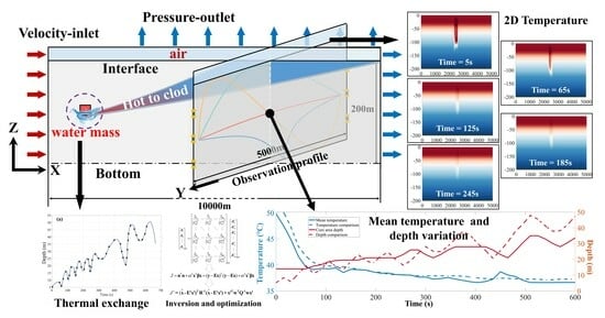
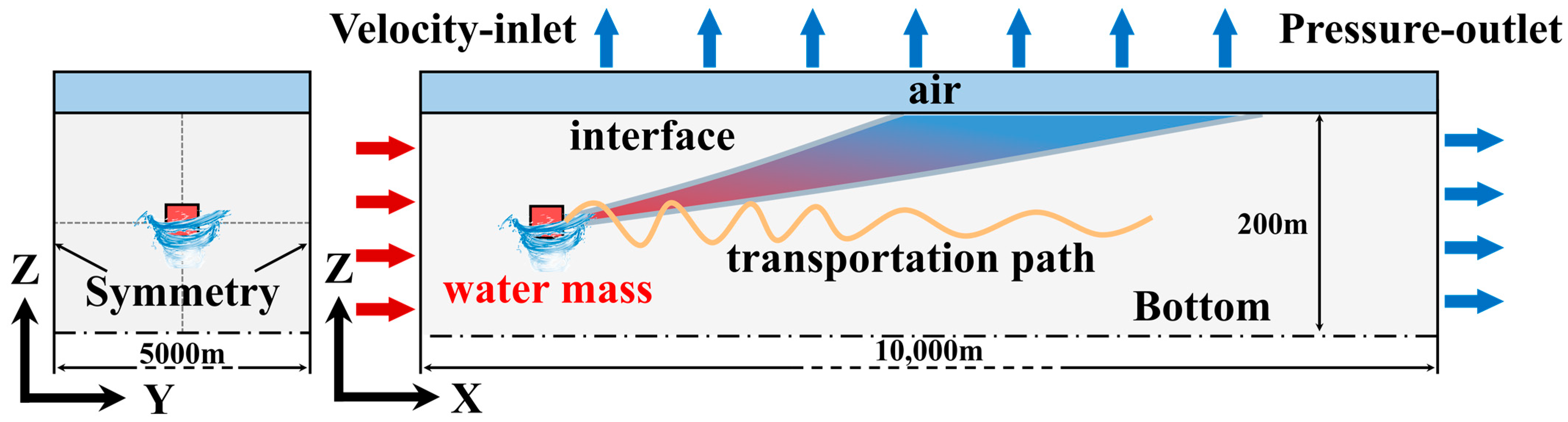
2. Simulation Model and Method

In this section, a numerical simulation model of the hot water mass flotation and diffusion by multiphase flow model is introduced in Section 2.1. Then the simulation of acoustic signal transmission is conducted based on the numerical simulation. In addition, an inversion and optimization method for reconstructing water temperature variations based on reasonable CAT station design is presented in Section 2.2 and Section 2.3.

2.1. Simulation Model

The numerical simulation setting of hot water mass transportation is shown at Figure 1. This paper mainly studies the floatation and diffusion process of the hot water mass along the transportation route, which means numerical simulation supplies the water temperature variation to the signal transmission. The signal travel time will change under the hot water mass transportation.

The size of the water mass in the simulation model is about 50 m × 50 m. The water mass motion route simulation uses unstructured dynamic grids. The size of the computational domain set as 10,000 m × 5000 m × 200 m (the X-axis direction is the direction of water mass motion, the Y-axis is the direction of water mass radial motion and the Z-axis is the water depth direction). The fluid medium in this domain is seawater and the medium in the upper domain is air.

The boundary conditions include velocity inlet, pressure outlet, wall and interface. Velocity inlet: velocity is set as 0.1 m/s on the left-side surface towards the right-side surface of water mass (the positive direction of the X-axis); the preset temperature of water mass is set as 5 °C. Pressure outlet: set the static pressure value of right surface relative to the reference pressure (the reference pressure is 1 atmosphere). Wall: the surface of the bottom is set as a no-slip wall, the two surfaces of radial direction are set as symmetric walls, and interface between the seawater and air space is set as a free surface. Interface: the surface between water mass computational domain and external field computational domain is set as the interface surface. Overlap: an overlapping mesh area is set over the transportation route.

The numerical simulation model is carried out as follow. The water computational domain uses the refined unstructured grid, the external flow field computational domain uses the structured mesh to increase the accuracy. The interface and water temperature exchange regions are encrypted mesh to facilitate the detail variations of the hot water mass transportation process and characteristics. Based on the simulation, the theoretical mechanisms of water floatation and diffusion are formed from the water mass transportation. The simulation process and setting are only briefly described at this section. This paper places emphasis on observing the simulation results of hot water mass flotation and diffusion via acoustic tomography technology and discusses the feasibility of this.

2.2. Inversion Method

The water temperature variations caused by hot water mass flotation and diffusion influence the signal transmission in vertical profile. In other words, signal travel time will be influenced by the hot water mass transportation. The inversion problem is at the core for solving temperature variation based on the recorded travel time.

In the simulation, only the effect of temperature change is added, this paper focuses on temperature variations during floatation and diffusion processes of the hot water mass. It should be mentioned that the flow velocity is not studied in this paper, because the vertical ZY observation profile is perpendicular to the moving transportation route of hot water mass, which means the flow velocity variations can hardly affect the signal travel time. Two-way signal travel time is used for flow field study, so one-way signal travel time is enough for the inversion problem of water temperature. Figure 2 shows an acoustic simulation model of the station deployment and observation method.

The signal travel time along the sound ray path (l) is:

$$t={\displaystyle {\int }_l\frac{ds}{C_0(x,y,z)+\delta C(x,y,z)}}$$

(1)

where $C_0(x,y,z)$ is the reference sound speed in grid $(x,y,z)$ alone, $\delta C(x,y,z)$ is the sound speed deviation caused by water temperature changing, and l is the sound ray path of the signal transmission between each station pair (one sends a signal and one receives a signal). To simplify expression, station pair between each two-station mark with station depths as 50 m_50 m, 100 m_100 m and 150 m_150 m, e.g., 50 m_50 m denotes the transmission of two stations where both are at a depth of 50 m.

The reference travel time without temperature variation is:

$$t_0={\displaystyle {\int }_l\frac{ds}{C_0(x,y,z)}}$$

(2)

By Equations (1) and (2), the travel time deviation is formulated as:

$$\delta t={\displaystyle {\int }_l\frac{ds}{C_0(x,y,z)+\delta C(x,y,z)}}-{\displaystyle {\int }_l\frac{ds}{C_0(x,y,z)}}$$

(3)

Due to $C_0(x,y,z)\gg \delta C(x,y,z)$, by adopting the Taylor expansion of Equation (3), it reduces as:

$$\delta t={\displaystyle {\int }_l\frac{ds}{C_0}\left(1-\frac{\delta C}{C_0}+{\left(\frac{\delta C}{C_0}\right)}^2-{\left(\frac{\delta C}{C_0}\right)}^3\cdots \right)}-{\displaystyle {\int }_l\frac{ds}{C_0}}$$

(4)

The terms higher than the second order are extremely small and neglected in Equation (4), so we obtain:

$$\delta t\approx {\displaystyle {\int }_l\frac{ds}{C_0}\left(1-\frac{\delta C}{C_0}\right)}-{\displaystyle {\int }_l\frac{ds}{C_0}}=-{\displaystyle {\int }_l\frac{\delta C}{C_0^2}}ds$$

(5)

Based on Equation (5), we can study the sensitivity of the sound speed from signal travel time variations, which are caused by water temperature fluctuation. Along the sound speed equation $C(T,S,D)$ as in Equation (6) [19], generally, sound speed increases by about 4.5 m/s when the water temperature increases by 1 °C.

$$\begin{array}{cc}C(T,S,D)& =1448.96+4.591T-0.05304T^2+2.734\times {10}^{-4}{T}^3\\ & +1.340(S-35)+1.630\times {10}^{-2}D+1.675\times {10}^{-7}{D}^2\\ & -1.025\times {10}^{-2}T(S-35)-7.139\times {10}^{-13}T{D}^3\end{array}$$

(6)

Hot water mass flotation and diffusion exist in different phases [4,5,6]. The phase of hot water mixing with cold water and then rising upward and spreading out is the easiest stage to observe, here water temperature changes by about 0.2~1 °C [9,10].

Assuming an ideal environment, the reference sound speed is negative gradient, the water temperature increases by 0.5 °C after water mass transportation, and station-pair distance is about 5000 m. In this case, a 0.5 °C rise in temperature may lead to sound speed about 2.25 m/s increasing, which means travel time deviation is about 0.005 s by Equation (5). This result is based on the fact that the water temperature rises along the entire sound ray path. However, if the flotation or diffusion width of water mass is only 100 m, the travel time deviation is about 0.0001 s. In order to identify such small variations, acoustic signal sampling frequency of more than 10 k is required to identify travel time deviation. As per the above discussion, the hot water mass flotation and diffusion can be observed by high-frequency signal transmission. But high frequency exhibits higher signal attenuation which means shorter transmission distances. Thus, it is important to balance the signal sampling frequency and station-pair distances to obtain the water temperature variations.

In addition, in the inversion solution, the vertical profile is grid divided to match and identify the relevant sound ray paths for establishing the coefficient matrix. The travel time of sound ray path is affected when the ray path passes through the temperature changing grids during hot water mass transportation. Thus, the direct inversion method cannot capture changes in detail, which means the partial variations of hot water mass are reflected in the whole vertical profile leading to distortion of the inversion results. Therefore, the mode rule of floatation and diffusion process of the hot water mass is added in the inversion process to optimize the results.

Matrix relationships are established according to Equation (5) as follow:

$${\left[\begin{array}{c}\delta t_1\\ \delta t_2\\ ⋮\\ \delta t_n\end{array}\right]}_{n\times 1}=-{\left[\begin{array}{ccccc}\frac{L_{11}}{{\left(C_0^1\right)}^2}& \cdots & \frac{L_{1j}}{{\left(C_0^j\right)}^2}& \cdots & \frac{L_{1m}}{{\left(C_0^m\right)}^2}\\ ⋮& \ddots & ⋮& \ddots & ⋮\\ \frac{L_{i1}}{{\left(C_0^1\right)}^2}& \cdots & \frac{L_{ij}}{{\left(C_0^j\right)}^2}& \cdots & \frac{L_{im}}{{\left(C_0^m\right)}^2}\\ ⋮& \ddots & ⋮& \ddots & ⋮\\ \frac{L_{n1}}{{\left(C_0^1\right)}^2}& \cdots & \frac{L_{nj}}{{\left(C_0^j\right)}^2}& \cdots & \frac{L_{nm}}{{\left(C_0^m\right)}^2}\end{array}\right]}_{n\times m}{\left[\begin{array}{c}\delta C_1\\ \delta C_2\\ \delta C_3\\ ⋮\\ \delta C_j\\ ⋮\\ \delta C_m\end{array}\right]}_{n\times 1}$$

(7)

where j denotes the jth grid, where Equation (7) is written as the following formula [20,21]:

$$\mathbf{y}=\mathbf{E}\mathbf{x}+\mathbf{q}$$

(8)

where $y=\left\{\delta t_i\right\}$ is the travel time deviation vector, $E=\left\{E_{ij}\right\}=\left\{L_{ij}/{\left(C_0^j\right)}^2\right\}$ is the transform matrix, $x=\left\{\delta C_j\right\}$ is the unknown variable vector, and $q=\left\{q_j\right\}$ is the solution error vector, n is the ray number and m is the grid number.

Equation (8) is solved by regularized inversion with tapered least square method, in which the objective function J is given as:

$$J=n^{T}n+{\alpha }^2{x}^T\beta x={(y-Ex)}^T(y-Ex)+{\alpha }^2{x}^T\beta x$$

(9)

where $\alpha$ is the damping factor and $\beta$ is the matrix of regular coefficients evolving from the water mass mode rule. The expected solution of x is determined to minimize the objective function J:

$$\widehat{x}={\left(E^{T}E+{\alpha }^2\beta \right)}^{-1}{E}^{T}y$$

(10)

By introducing singular value decomposition, the E matrix is decomposed as:

$$E={\displaystyle \sum _{k=1}^{N_k}{\lambda }_k}{u}_k{v}_k^T=U\Lambda V^T$$

(11)

where $U=\left[u_1,u_2,u_3,\cdots ,u_{N_k}\right]$, $V=\left[v_1,v_2,v_3,\cdots ,v_{N_k}\right]$ and

$$\Lambda =\left[\begin{array}{ccccc}{\lambda }_1& \cdots & 0& \cdots & 0\\ ⋮& \ddots & ⋮& \ddots & ⋮\\ 0& \cdots & {\lambda }_{N_k}& \cdots & 0\\ ⋮& \ddots & ⋮& \ddots & ⋮\\ 0& \cdots & 0& \cdots & 0\end{array}\right]$$

(12)

where $N_k$ is the number of nonzero singular values. The weighting matrix $\beta$ is introduced to weaken the influence of the unchanged grids and to increase the weights of the changed grids at different depths according to the mode rules of hot water mass transportation, and is formulated as:

$$\beta =\left[\begin{array}{cccccccc}{\beta }_1& 0& 0& 0& 0& 0& 0& 0\\ 0& 1& 0& 0& 0& 0& 0& 0\\ 0& 0& 1& 0& 0& 0& 0& 0\\ ⋮& ⋮& ⋮& \ddots & ⋮& ⋮& ⋮& ⋮\\ 0& 0& 0& 0& {\beta }_j& 0& 0& 0\\ ⋮& ⋮& ⋮& ⋮& ⋮& \ddots & ⋮& ⋮\\ 0& 0& 0& 0& 0& 0& 1& 0\\ 0& 0& 0& 0& 0& 0& 0& {\beta }_{\mathrm{m}}\end{array}\right]$$

(13)

Different kinds of weighting factors (1, ${\beta }_1$, ${\beta }_2$, …, ${\beta }_m$) are allocated for the central grids including mixing grids, side grids and diffusion grids. ${\beta }_j=1$ denotes the grid j where sound ray paths do not pass through. The size of weighting factors in different grids is determined by the hot water mass mode. Here, this mode is obtained from the numerical simulation.

By using Equations (10)–(13), the equation is rewritten:

$$\widehat{x}={\displaystyle \sum _{i=1}^{N_k}\frac{{\lambda }_i{u}_i^T{v}_{i}y}{{\lambda }_i^2+{\alpha }^2{\beta }_i}}$$

(14)

The expected solution error vector becomes:

$$\widehat{n}=y-E\widehat{x}=\left\{I-E{\left(E^{T}E+{\alpha }^2\beta \right)}^{-1}{E}^T\right\}y$$

(15)

The error of the expected solution becomes:

$${\widehat{x}}_{error}={\left(E^{T}E+{\alpha }^2\beta \right)}^{-1}{E}^T\widehat{n}$$

(16)

Note that, the damping factors $\alpha$ is calculated by the L-curve method [22]. $\alpha$ and $\beta$ are updated at every signal transmission. We define the inversion result obtained when L-curve is fold at the maximum curvature point. Thus, this method provides flexibility to reconstruct flotation and diffusion processes of hot water mass.

2.3. Optimization of Vertical Results

The inversion results are obtained via the proposed method in the Section 2.3. But the observation area always exists acoustic shadow zone, which means the inversion results based on mode rule are sparse results (the results of ray path not pass through grid is 0). Although the inversion method smooths the results by the matrix of regular coefficients ($\beta$). It improves the results quality, but it does not optimize the sparse region. Thus, a model assimilation is introduced to further improve the accuracy of the inversion results.

Referring state estimation optimization methods, the new optimization loss function is established as follow:

$$J^{\prime }={(\widehat{x}-E^{\prime }{x}^{\prime })}^T{R}^{-1}(\widehat{x}-E^{\prime }{x}^{\prime })+{{\mathbf{x}}^{\prime }}^{\mathbf{T}}x{w}^T{Q}^{-1}w{x}^{\prime }$$

(17)

where $\widehat{x}$ is the grided inversion results in vertical profile, $E^{\prime }$ is the grid distance relationship matrix between gird and sound rays, R is the covariance matrix of the inversion error, Q is the covariance matrix of the model (background) error, w is the grided model (background) results. The inversion error controls the accuracy of the inversion results, and the model error controls the error in the unfitted region, which inversion error has a dominant effect on inversion results

The model (background) results are the data of numerical simulation. For example, the hot water mass flotation and diffusion simulation give the background water temperature variations at different moments, in other words it gives the reference water temperature at different grids. By this, the whole vertical profile results can be further optimized and improved.

From Equation (17), the local minimum value can be expressed as:

$${\widehat{x}}^{\prime }={\left({{\mathbf{E}}^{\prime }}^{\mathbf{T}}{R}^{-1}{E}^{\prime }+w^T{Q}^{-1}w\right)}^{-1}{{\mathbf{E}}^{\prime }}^{\mathbf{T}}{R}^{-1}\widehat{x}$$

(18)

The expected solution error vector and uncertainty of the solution can be expressed as:

$${\widehat{n}}^{\prime }=\left\{I-E^{\prime }{\left({{\mathbf{E}}^{\prime }}^{\mathbf{T}}{R}^{-1}{E}^{\prime }+w^T{Q}^{-1}w\right)}^{-1}{E^{\prime }}^{\mathbf{T}}{R}^{-1}\right\}\widehat{x}$$

(19)

$$\begin{array}{c}p={\left({{\mathbf{E}}^{\prime }}^{\mathbf{T}}{R}^{-1}{\mathbf{E}}^{\prime }+{\mathbf{w}}^{\mathbf{T}}{Q}^{-1}w\right)}^{-1}{{\mathbf{E}}^{\prime }}^{\mathbf{T}}{R}^{-1}〈{\widehat{n}}^{\prime }{{\widehat{n}}^{\prime }}^{\mathbf{T}}〉\\ R^{-1}{\mathbf{E}}^{\prime }{\left({{\mathbf{E}}^{\prime }}^{\mathbf{T}}{R}^{-1}{\mathbf{E}}^{\prime }+{\mathbf{w}}^{\mathbf{T}}{Q}^{-1}w\right)}^{-1}\end{array}$$

(20)

The whole vertical profile results are reconstructed by the inversion results and model (background) results.

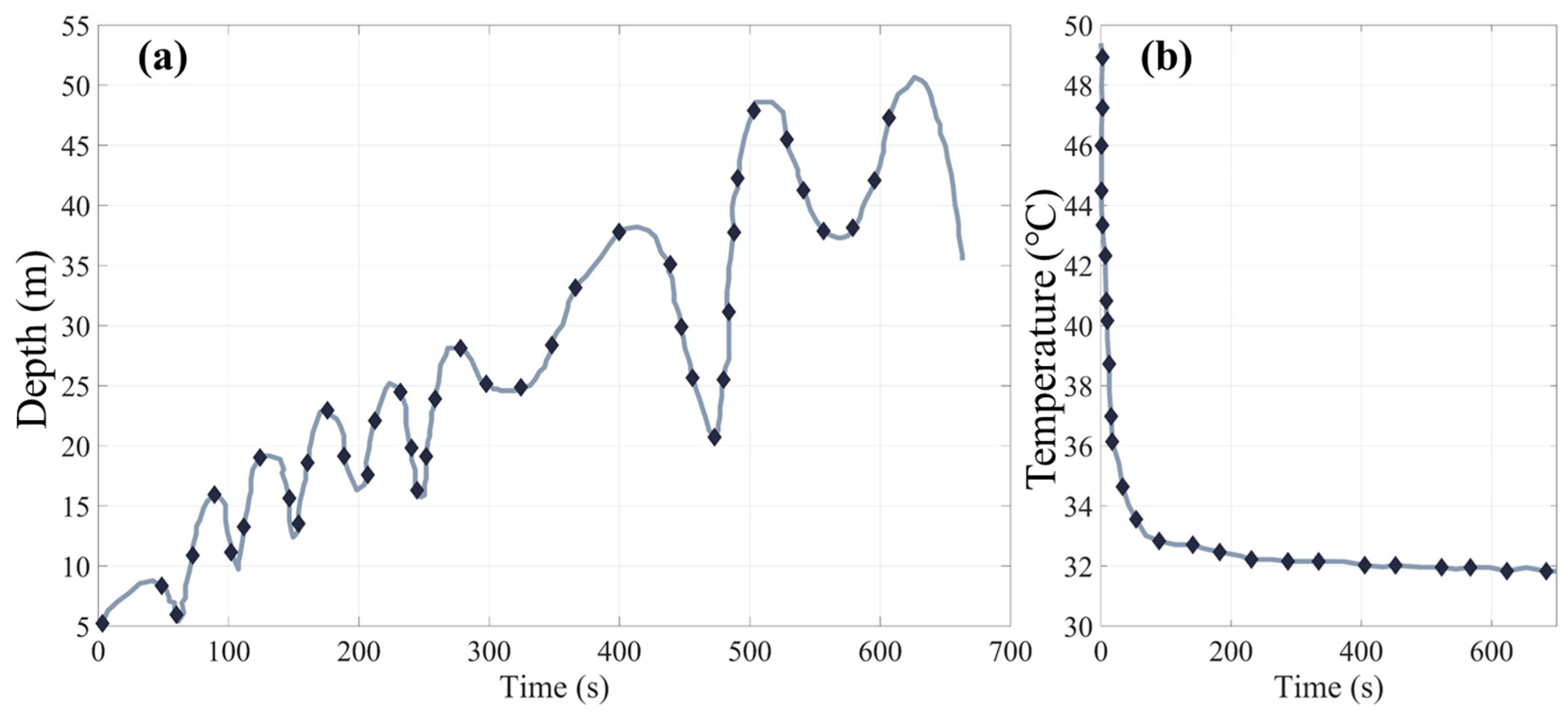
3. Thermal Exchange and Signal Identification

As per the introduction, the numerical simulation builds a background hot water mass field, and then an acoustic transmission simulation based on numerical simulation is performed. Figure 2 shows an acoustic tomography observation model of flotation and diffusion of hot water mass. We defined the observation profile on the ZY plane at the position of x = 0, where the hot water mass begins to float and diffuse (thermal exchange). The core area in Figure 2 is the main region of variation in water temperature, where sound rays are concentrated at depths of 100 m. In real observation experiments, it is not possible to real-time record the fluctuation of water temperature due to the signal interval between signal sending and receiving. In the early stage of the thermal exchange, the sudden water temperature change cannot be distinguished via acoustic signal. So, we place emphasis on the flotation and diffusion of hot water mass mixing with seawater phase and record the water temperature variations via signal transmission. Note that, only the water temperature variations are observed and studied here, and the most obvious stage is the process of water temperature stabilization during the floating and diffusing phases.

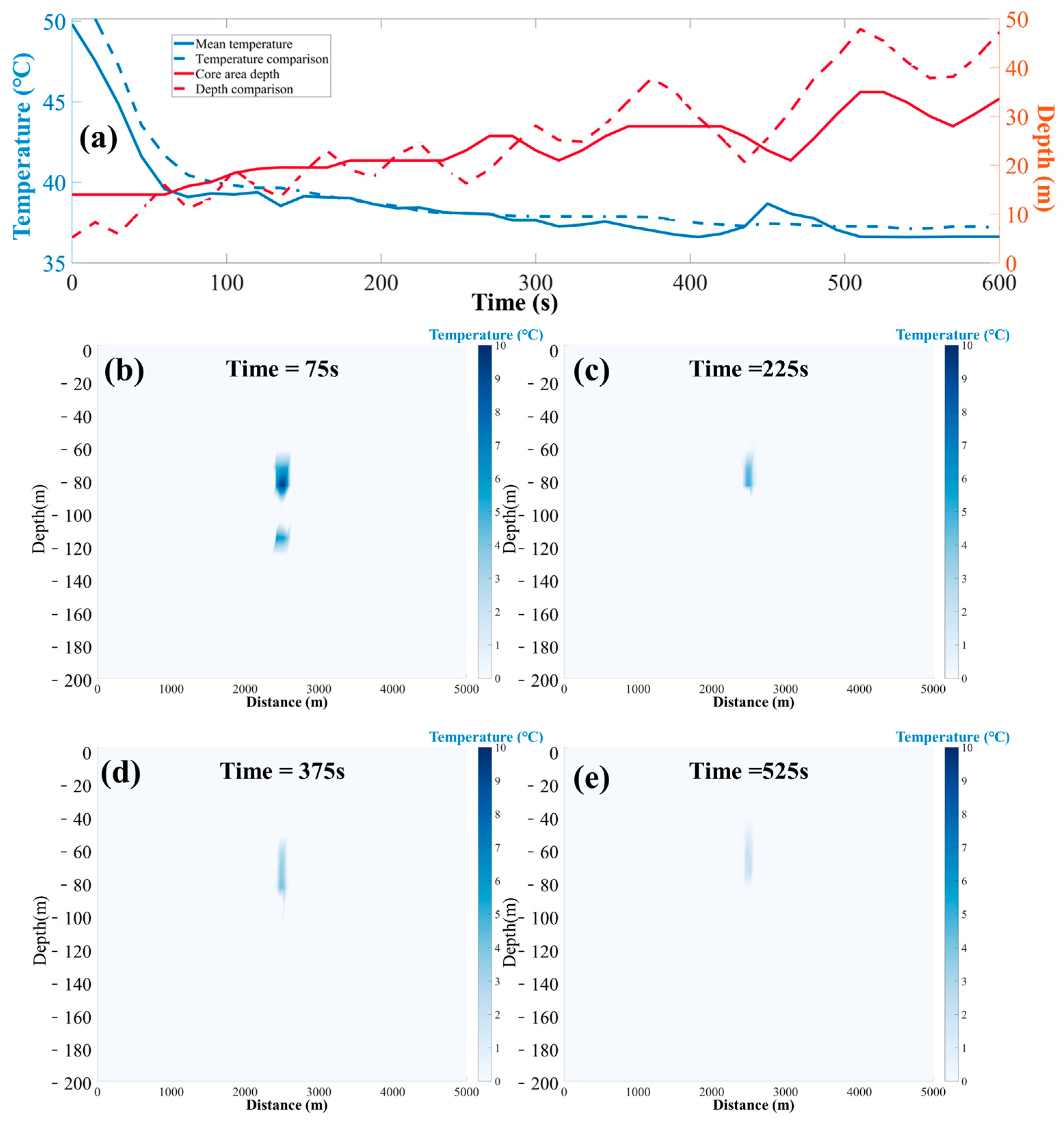
3.1. Thermal Exchange

Figure 3 shows the numerical simulation results of flotation and diffusion of the hot water mass. It shows the variation of the maximum floating height at position x = 0 and the decay rule of the temperature variations at a depth of 100 m and time = 0. Time = 0 is the moment the hot water mass begins thermal exchange.

Figure 3a shows the mode rule of maximum floating height with time after the hot water mass transportation, where the hot water mass exchanges with the cold seawater. In the early stage, the initial floating velocity of hot water mass is fast and the fluctuation amplitude is small. In the later stage, the floating velocity of hot water mass gradually slows down and the range of fluctuations becomes larger. The reason for this is that the hot water mass has not been fully diffused and the larger temperature difference generates the smooth rise of the hot water mass in initial phase. However, over time, the temperature difference is weakened and the diffusion is more adequate and the floatation process of the hot water mass produces more intense oscillations.

The decay rule of the temperature variations at depth of 100 m, x = 0 is shown in Figure 3b. It can be seen that the large water temperature difference occurs in the early phase, where the center temperature rapidly declines due to the hot water mass mixing with cold water. Then, the intensity of the water thermal exchange rapidly declines and the center temperature slows down as the temperature difference decreases.

Through the analysis of Figure 3, we can deduce the two mode rules of maximum floating height and water temperature variations in the core area. This is then extended to changing vertical profile grids to establish the weighting matrix $\beta$ and background results. Among them, the maximum floating height of hot water mass varies regularly with time and water temperature at the core area is gradually consistent with the ambient temperature. In summary, we obtained the flotation and diffusion rule of the hot water mass and the water temperature distribution results in the vertical profile. After converting water temperature into sound speed, the effected profile is used for simulating the acoustic signal transmission at different moments.

3.2. Signal Identification in Acoustic Transmission Simulation

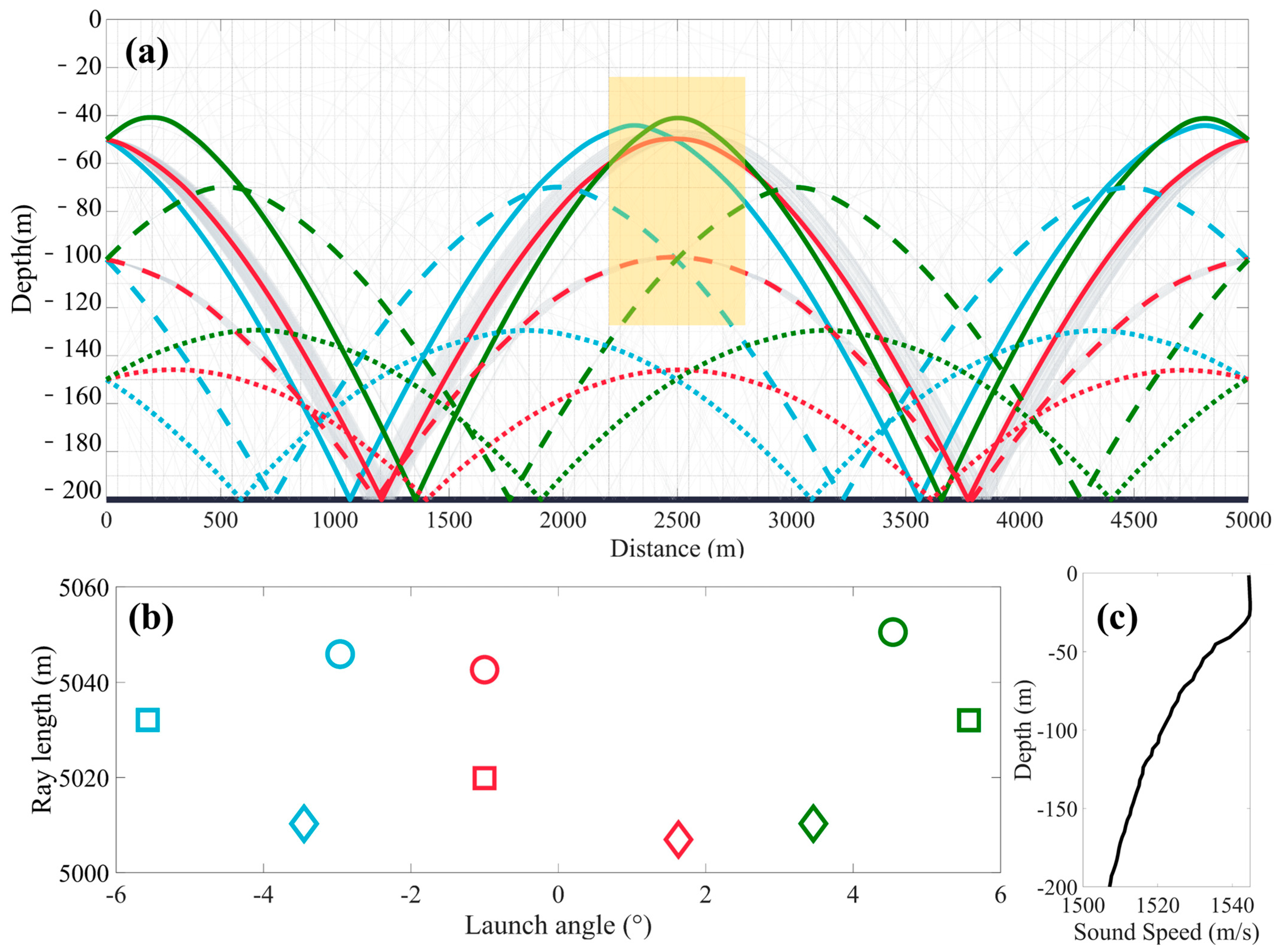
Sound signal identification is the distinguishing and matching of sound ray paths corresponding to travel times based on sound ray simulation. Firstly, original acoustic transmission simulation without the influence if hot water mass transportation is carried out to identify original sound rays. Then, the affected ray simulations are performed at different moments with variations of water temperature environment. From Figure 3, it can be seen that hot water mass is mainly in the middle depth layer in the initial phase, in which the sound rays in upper and lower station pairs (50 m_50 m and 150 m_150 m) are not greatly influenced. As the hot water mass begins gradually floating and diffusing, it has an effect on the sound rays of the upper station pair.

In this acoustic transmission simulation, only two stations at the same depth are carried out across a distance of 5000 m, defined as 50 m_50 m, 100 m_100 m and 150 m_150 m. The ray simulation between different depths such as 50 m_150 m cannot identify effective ray (sound ray in acoustic channel) paths due to the complex acoustic channel. Our previous experimental experience also shows that station pairs at the same depth are easier for acoustic signal transmission [21].

In this simulation, the terrain is simplified with a depth of 200 m. Thus, the original acoustic transmission simulations are first identified by three sound ray paths of three station pairs, as shown in Figure 4. The identified ray paths divide in grids as in Figure 4a. Figure 4a shows the original simulation results of 50 m_50 m, 100 m_100 m and 150 m_150 m, represented by solid lines, dashed lines, and dotted lines, respectively. The green, red, and blue lines represent different travel times of sound rays which are bottom reflected more than once. The circles, squares and diamonds in Figure 4b show the relationship between ray length and launch angle of three station pairs.

Table 1. Original acoustic transmission simulation of identified rays.

Station Pairs	Launch Angle (°)	Ray Length (m)	Travel Time (s)
50 m_50 m	−2.96 (blue ray)	5045.919590	3.3144957
	−1 (red ray)	5042.638983	3.314263
	4.54 (green ray)	5050.544503	3.314902
100 m_100 m	−5.57 (blue ray)	5032.079960	3.3136260
	−1 (rad ray)	5019.860809	3.3125639
	5.57 (green ray)	5032.025004	3.313598
150 m_150 m	−3.45 (blue ray)	5010.278219	3.312462
	1.63 (rad ray)	5006.951102	3.312726
	3.46 (green ray)	5010.304894	3.312469

shows the detail results of identified rays in the original simulation.

As the identification of the affected ray simulation is influenced by hot water mass transportation, the sound ray paths with the same launch angles as in the original simulation are selected. Thus, the travel time variations in the affected ray simulation can be assumed to be caused by the influence of the hot water mass flotation and diffusion.

It is important to note that the selected ray paths are based on whether the sound rays pass through the core area or not (core area is the yellow area in Figure 4). Due to terrain depth and distance limitations, there is no direct ray, only bottom reflected ray paths are identified. In the real experiment, bottom reflection produces a large attenuation to the acoustic signal. The sound speed profile under the influence of hot water mass transportation is varied not only in the depth direction (Z-axis), but also in the horizontal direction (Y-axis). The travel time of ray paths is changing due to this influence in the grided vertical profile.

4. Results

In this section, travel time variations are shown in Figure 5. The behaviors of the flotation and diffusion of hot water mass in the simulation are reconstructed and demonstrated via inversion and optimization method. Figure 6 and Figure 7 show the results by grid-averaged variations and the error of the result. Then, the comparison between real results and inversion optimization results is introduced, and the water mass transportation route based on inversion and optimization is discussed.

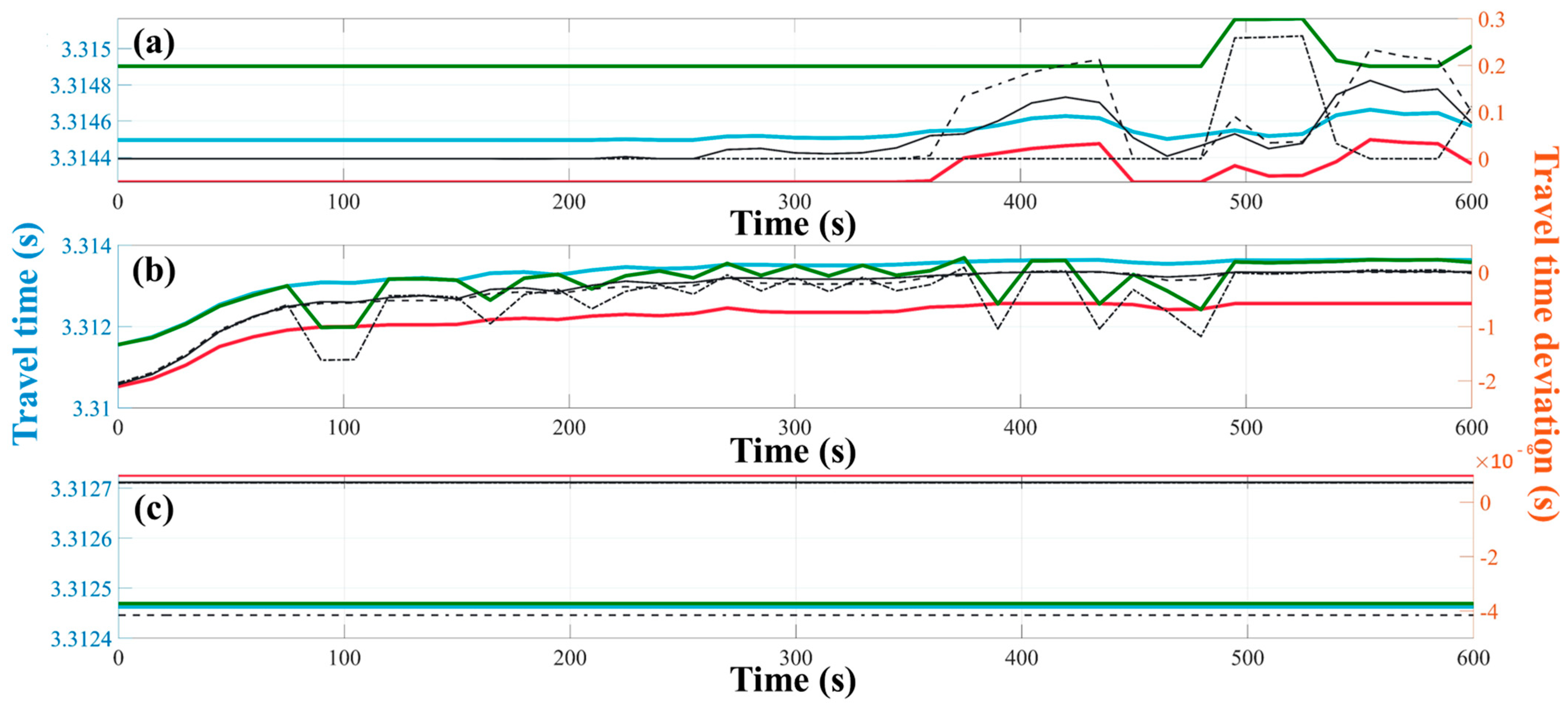
4.1. Travel Time Variation

The travel time variations of sound ray paths at each station pair in hot water mass acoustic transmission simulation and travel time deviation (simulated travel time minus original travel time) are shown in Figure 5. In Figure 5, the X-axis is the time, the left Y-axis is the travel time, and the right Y-axis is the travel time deviation. Figure 5a–c denote the simulation results of three station pairs, 50 m_50 m, 100 m_100 m and 150 m_150 m. The red, green and blue curves are travel time changes over time, and the curves of the travel time variations in different colors correspond to the identified sound rays in Figure 4a. The black lines with different line types represent the travel time deviation variations over time, where the solid, dashed, and dotted lines denote the blue ray, red ray, and green ray, respectively. The original acoustic transmission simulation of identified rays between three station pairs are shown in Table 1.

Firstly, we focus on the core area in the hot water mass transportation (yellow area in Figure 4a) at a depth of 100 m, which corresponds to the curves in Figure 5b. From Figure 5b, the sound ray paths’ travel time fluctuates significantly as the hot water mass floats. The most obvious variation is the green ray, which indicates this sound ray is greatly affected by the water temperature variations. The reason for this is that the green ray passes through a longer distance in the core observation area, in other words, the temperature fluctuation of hot water mass creates a larger impact on it. In contrast, the red and blue rays show less changes. In addition, the travel time of three sound rays gradually slows down. Especially in the first 50 s, the travel time increase fast. From the variations of black curves, it can be seen that the mean value of travel time deviation is about 1 ms. Based on Equation (5) and the size of the core observation area, the sound speed difference caused by 1 ms of travel time deviation has an effect of about 0.5 m/s (caused by the temperature changes of hot water mass exchange).

Figure 5a is the travel time results of a station pair at a depth of 50 m. Compared to Figure 5b, there are no significant variations in the curves at the first 350 s phase, after which the travel time curves fluctuate significantly. Due to the thermal exchange of hot water mass, it has no influence on the signal transmission of the upper sound ray path layer in the beginning. Then, the travel time changes with the effect of the hot water mass flotation and diffusion, similar to the maximum floating height shown in Figure 3a. The travel time deviation in Figure 5a is smaller than that in Figure 5b, in which the mean travel time deviation in Figure 5b is about 20 ms (about 10 m/s sound speed difference of the floating core observation area). Figure 5c is basically unchanged, which is due to the fact that the thermal exchange of hot water mass did not affect the acoustic transmission of the station pair at a depth of 150 m.

The summarized rules from travel time and travel time deviation over time from the above simulation results are as follows: the hot water mass initially affects the core observation area at a depth of 100 m and immediately produces a large decay. As the hot water mass floats, the core observation area is diffusing, and station pairs at shallow depths are influenced. On the other hand, the station pair at a depth of 150 m is unchanged. In comparison, travel time deviation in the station pair at a depth of 100 m is significant, which indicates the larger sound speed difference caused by water temperature variations during hot water mass transportation.

The sound speed difference in acoustic simulation is solved by the travel time deviation via the proposed inversion and optimization method in the core observation area. Thus, the variation range of the sound speed is calculated, which is used to further solve the variation range of water temperature influencing the hot water mass to validate the rules of floatation and diffusion.

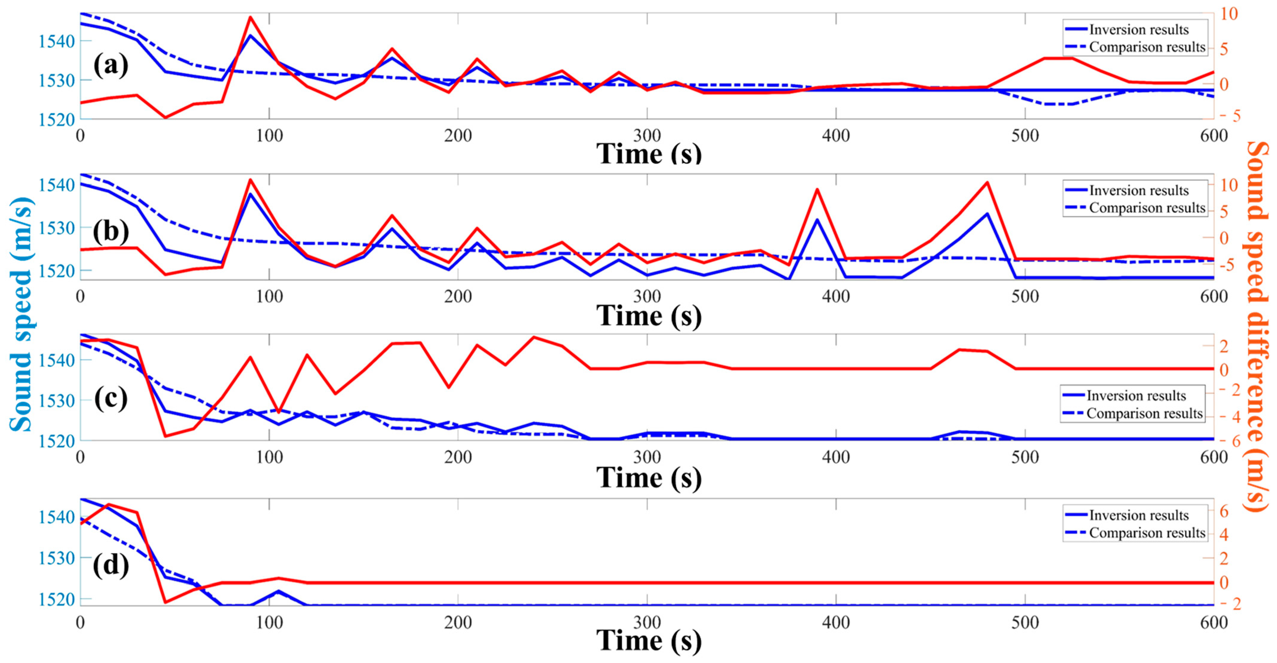
4.2. Inversion and Optimization Results

The temperature and sound speed inversion and optimization results via the travel time deviation are shown at Figure 6 and Figure 7. Figure 6 shows the variations of two-dimensional (2D) temperature inversion and optimization results at vertical profile from 5 s to 515 s with intervals of 30 s, which display the basic rule of hot water mass flotation and diffusion in the core observation area. The X-axis is the distance, Y-axis is the depth, and the color is the temperature value. Note that the water temperature in the entire 2D vertical profile is obtained through grid interpolation of inversion and optimization results.

In addition, Figure 7 shows the results of sound speed and sound speed difference over time at depths of 75 m, 95 m, 115 m and 135 m. In Figure 7, X-axis is the time, the left Y-axis is the sound speed, and the right Y-axis is the sound speed difference. The two blue curves are speed sound variations, in which solid curves represent inversion optimization results and dashed curves represent comparison results (numerical simulation results). Red curves represent the variations of sound speed difference between the inversion optimization results and the numerical simulation results.

From the 2D temperature profile inversion and optimization results in Figure 6, it can be seen that water temperature changes in the core area are clearly different from the background water environment. It demonstrates that the additional matrix and model correlation matrix can effectively regularize grided results and obtain the sound speed variations in the inversion and optimization method. From 5 s to 500 s, the water temperature increases are particularly significant in the initial stage, but in the later stage, the water temperature gradually becomes the same as the background environment temperature. However, the trend of increasing temperatures in the core observation area is not obvious.

Figure 7 shows the sound speed variation at four different depth grid positions, which can also be regarded as the water temperature variation. It basically reveals the process of water variation at different depths during the hot water mass flotation and diffusion. Combining the Figure 7a–d, the sound speed dropping in the beginning stage, but eventually it fluctuates around the background water temperature and gradually stabilizes. Moreover, the sound speed fluctuations near the core observation area in Figure 7b,c are more significant. Furthermore, the numerical simulation fluctuation patterns are similar with the variations of inversion results in Figure 7.

From Figure 6 and Figure 7, the inversion and optimization results preliminarily validate the observation of the hot water mass variation via acoustic tomography technology. The rules of the hot water mass transportation in 2D vertical profile are obtained. Through comparison, the trend of inversion optimization results and numerical simulation results are similar, but error via inversion and optimization results still exist due to the algorithmic overfitting.

4.3. Comparison

The sound speed difference in Figure 8 is the sound speed inversion and optimization results compared with the sound speed in original results. The X-axis is the time, left Y-axis is the temperature variation and right Y-axis is the depth variation. Blue solid curve is the mean temperature in core observation grids and blue dashed curve is the water temperature comparison. The red solid curve is the depth variation of the core area and the red dashed curve is the depth comparison between inversion optimization results and numerical simulation results.

The RSMEs (Root Mean Square Error) in Figure 7a–d at four different grid depths are 3.72 m/s, 4.61 m/s, 1.80 m/s and 1.585 m/s respectively. And the mean RSME in the whole 2D vertical profile is 2.23 m/s. A larger sound speed difference exists in the beginning, which means the difference is large during the hot water mass mixing with seawater at first. In inversion and optimization problems, this difference will cause a cumulative fitting inversion error. However, the sound speed difference is still within the controllable range and does not exceed the pre-set value.

Figure 8 shows the comparison of the temperature variation and maximum floating depth variation at the core area. It shows the change of temperature floatation and diffusion in 2D vertical profiles at four different moments. This comparison also shows that the inversion and optimization results are basically consistent with the simulation, which means the feasibility of monitoring the flotation variation of the water mass transportation route via acoustic tomography. However, the accuracy of the results does not reach a very satisfying condition, which is discussed in Section 5.

5. Discussion

The 2D station observation design at the vertical profile effectively establishes water mass transportation routes of water temperature variation through the signal travel time. In particular, the advantage of acoustic tomography observation technology is high sensitivity and high perceptibility for real-time monitoring 2D water temperature field via acoustic transmissions. In this paper, the flotation and diffusion numerical simulation model and acoustic transmission simulation model are used to discuss the thermal exchange of hot water mass in a 2D vertical profile.

If multiple cross vertical profiles and multiple acoustic stations are established to monitor the water temperature variation of the hot water mass, it will improve the accuracy of thermal exchange observation. Moreover, the acoustic signal travel time deviation is not only used to establish the water temperature observation, but also the travel time difference can be further used to establish the flow velocity variation. It is also an important way to monitor state of hot water mass transportation.

However, there are some shortcomings in the acoustic tomography observation technology. Due to the water temperature variation in the real experiment environment being potentially much smaller than the simulation model, it is extremely important to design and set the suitable station-pair distance for high-frequency acoustic signal transmission. Meanwhile, the simulation model established in this paper is focused on the core observation area of 2D vertical profile. However, the floating and diffusing position of hot water mass in reality is randomly distributed. The 2D vertical profile may be inclined and elevated with the flotation and diffusion motion of hot water mass. Thus, establishing an effective acoustic tomography observation mode matrix and corresponding high-precision inversion and optimization methods on specific hot water mass transportation experiments is important preprocessing. Furthermore, it also needs to solve the problem of obtaining the basic motion of hot water mass. As for the station drift, the station position has a significant impact on acoustic tomography observations of water temperature. In real observations, stations may drift due to the influence of currents and this problem is solved by secondary localization or drift correction algorithms.

Acoustic tomography is a common way for underwater temperature and flow field observation in areas, such as oceans and rivers. Acoustic tomography has unique observational advantages for dynamic ocean processes such as water thermocline variations, internal wave transformations and so on. In this paper, the simulation model is established to briefly discuss the feasibility of using acoustic tomography to observe the flotation and diffusion of hot water mass. The water temperature and max floating height variation solved via the inversion and optimization method to verify whether the flotation and diffusion rule of hot water mass can be obtained. This put forward a reference construction for the subsequent research. In summary, the acoustic tomography technique is likely to observe the hot water mass transportation, but still needs further experimental verification.

6. Conclusions

The application of underwater acoustic tomography technology in the flotation and diffusion of hot water mass transportation observation is innovative research. A hot water mass transfer simulation and acoustic transmission simulation are conducted in this paper. The temperature (sound speed) variation of hot water mass in 2D vertical profile is successfully obtained via the proposed inversion and optimization method. The travel time in signal transmission by acoustic tomography is influenced during the floating and diffusing of hot water mass. The accuracy of the new method for observing the hot water mass transportation is compared and discussed.

We can summarize as follows:

• The sound speed of RSMEs between simulation results and inversion optimization results at whole core observation area is 2.23 m/s (equivalent to 0.4 °C temperature change), which is less than the error requirements. Furthermore, the curves fluctuations input and results are close and similar.
• The new proposed methods combined inversion and optimization, are based on the simulated hot water mass mode matrix, and are successfully used in the observation. The accuracy of results is verified the method effect.
• The signal transmission can be influenced by the hot water mass flotation and diffusion. Due to the small water temperature variation, the station deployment needs to consider the relationship between the signal loss and transmission distance.
• The application of acoustic tomography is an innovative way for thermal exchange observation, which is proved by the simulation comparison. The real sea scale variation needs further study and verification.

Hot water mass monitoring based on the underwater acoustic tomography is a practical method. Whether it can be applied maturely needs further verification and experiment. For this reason, we propose that the application of acoustic tomography to monitor hot water mass variation is a relatively new research direction.

References

1. Pearce, A.F.; Feng, M. The rise and fall of the “marine heat wave” off Western Australia during the summer of 2010/2011. J. Mar. Syst. 2013, 111, 139–156. [Google Scholar] [CrossRef]
2. Hobday, A.J.; Alexander, L.V.; Perkins, S.E.; Smale, D.A.; Straub, S.C.; Oliver, E.C.J.; Benthuysen, J.A.; Burrows, M.T.; Donat, M.G.; Peng, M.; et al. A hierarchical approach to defining marine heatwaves. Prog. Oceanogr. 2016, 141, 227–238. [Google Scholar] [CrossRef]
3. Scannell, H.A.; Johnson, G.C.; Thompson, L.; Lyman, J.M.; Riser, S.C. Subsurface Evolution and Persistence of Marine Heatwaves in the Northeast Pacific. Geophys. Res. Lett. 2020, 47, 10. [Google Scholar] [CrossRef]
4. Benthuysen, J.A.; Oliver, E.C.J.; Feng, M.; Marshall, A.G. Extreme Marine Warming Across Tropical Australia during Austral Summer 2015–2016. J. Geophys. Res.-Oceans 2018, 123, 1301–1326. [Google Scholar] [CrossRef]
5. Han, W.Q.; Zhang, L.; Meehl, G.A.; Kido, S.; Tozuka, T.; Li, Y.L.; McPhaden, M.J.; Hu, A.X.; Cazenave, A.; Rosenbloom, N.; et al. Sea level extremes and compounding marine heatwaves in coastal Indonesia. Nat. Commun. 2022, 13, 12. [Google Scholar] [CrossRef] [PubMed]
6. Varela, R.; Rodriguez-Diaz, L.; de Castro, M.; Gomez-Gesteira, M. Influence of Eastern Upwelling systems on marine heatwaves occurrence. Glob. Planet. Chang. 2021, 196, 9. [Google Scholar] [CrossRef]
7. Gentemann, C.L.; Fewings, M.R.; Garcia-Reyes, M. Satellite sea surface temperatures along the West Coast of the United States during the 2014–2016 northeast Pacific marine heat wave. Geophys. Res. Lett. 2017, 44, 312–319. [Google Scholar] [CrossRef]
8. Oliver, E.C.J.; Benthuysen, J.A.; Darmaraki, S.; Donat, M.G.; Hobday, A.J.; Holbrook, N.J.; Schlegel, R.W.; Sen Gupta, A. Marine Heatwaves. In Annual Review of Marine Science; Carlson, C.A., Giovannoni, S.J., Eds.; Annual Review of Marine Science; Annual Reviews: Palo Alto, CA, USA, 2021; Volume 13, pp. 313–342. [Google Scholar]
9. Chen, Z.Y.; Shi, J.; Li, C. Two types of warm blobs in the Northeast Pacific and their potential effect on the El Nino. Int. J. Climatol. 2021, 41, 2810–2827. [Google Scholar] [CrossRef]
10. Wang, Q.; Zhang, B.; Zeng, L.L.; He, Y.K.; Wu, Z.W.; Chen, J. Properties and Drivers of Marine Heat Waves in the Northern South China Sea. J. Phys. Oceanogr. 2022, 52, 917–927. [Google Scholar] [CrossRef]
11. Munk, W.; Wunsch, C. Ocean acoustic tomography—Scheme for large-scale monitoring. Deep. Sea Res. Part A Oceanogr. Res. Pap. 1979, 26, 123–161. [Google Scholar] [CrossRef]
12. Cornuelle, B.; Munk, W.; Worcester, P. Ocean acoustic tomography from ships. J. Geophys. Res. Oceans 1989, 94, 6232–6250. [Google Scholar] [CrossRef]
13. Shang, E.C.; Wang, Y.Y. Acoustic travel time computation based on pe solution. J. Comput. Acoust. 1993, 1, 91–100. [Google Scholar] [CrossRef]
14. Behringer, D.; Birdsall, T.; Brown, M.; Cornuelle, B.; Heinmiller, R.; Knox, R.; Metzger, K.; Munk, W.; Spiesberger, J.; Spindel, R.; et al. A demonstration of ocean acoustic tomography. Nature 1982, 299, 121–125. [Google Scholar] [CrossRef]
15. Zhang, C.Z.; Kaneko, A.; Zhu, X.H.; Gohda, N. Tomographic mapping of a coastal upwelling and the associated diurnal internal tides in Hiroshima Bay, Japan. J. Geophys. Res. Oceans 2015, 120, 4288–4305. [Google Scholar] [CrossRef]
16. Xu, S.J.; Li, G.M.; Feng, R.D.; Hu, Z.L.; Xu, P.; Huang, H.C. 3-D Water Temperature Distribution Observation via Coastal Acoustic Tomography Sensing Network. IEEE Trans. Geosci. Remote Sens. 2023, 61, 18. [Google Scholar] [CrossRef]
17. Kawanisi, K.; Bahrainimotlagh, M.; Al Sawaf, M.B.; Razaz, M. High-frequency streamflow acquisition and bed level/flow angle estimates in a mountainous river using shallow-water acoustic tomography. Hydrol. Process. 2016, 30, 2247–2254. [Google Scholar] [CrossRef]
18. Chen, M.M.; Hanifa, A.D.; Taniguchi, N.; Mutsuda, H.; Zhu, X.H.; Zhu, Z.N.; Zhang, C.Z.; Lin, J.; Kaneko, A. Coastal Acoustic Tomography of the Neko-Seto Channel with a Focus on the Generation of Nonlinear Tidal Currents-Revisiting the First Experiment. Remote Sens. 2022, 14, 12. [Google Scholar] [CrossRef]
19. Mackenzie, K.V. Nine-term equation for sound speed in the oceans. J. Acoust. Soc. Am. 1981, 70, 807–812. [Google Scholar] [CrossRef]
20. Xu, S.J.; Li, G.M.; Feng, R.D.; Hu, Z.L.; Xu, P.; Huang, H.C. Tomographic Mapping of Water Temperature and Current in a Reservoir by Trust-Region Method Based on CAT. IEEE Trans. Geosci. Remote Sens. 2022, 60, 14. [Google Scholar] [CrossRef]
21. Xu, S.J.; Feng, R.D.; Xu, P.; Hu, Z.L.; Huang, H.C.; Li, G.M. Flow current field observation with underwater moving acoustic tomography. Front. Mar. Sci. 2023, 10, 11. [Google Scholar] [CrossRef]
22. Hansen, P.C. Analysis of discrete ill-posed problems of the L-curve. SIAM Rev. 1992, 34, 561–580. [Google Scholar] [CrossRef]
Figure 1. Numerical simulation model setting of hot water mass transportation. Red arrows denote direction of velocity inlet (only in water domain). Blue arrows denote direction of pressure outlet. The gradient of color from red to blue denotes the probably process of water mass flotation and diffusion changing (hot water to cold water). The yellow line denotes the probable water mass transportation route.
Remotesensing 16 01105 g001
Figure 2. Acoustic tomography observation and grid slice model. Six transducers are developed three left and three right at depth of 50 m, 100 m and 150 m. Water mass variation grids are set at a depth of 100 m. The ZX plane is the same as Figure 1.
Remotesensing 16 01105 g002
Figure 3. Numerical simulations of flotation and diffusion of hot water mass. (a) is the maximum floating height at position x = 0, (b) is the decay rule of the temperature variations at depth 100 m.
Remotesensing 16 01105 g003
Figure 4. Ray simulation and identification. (a) ray simulations of 50 m_50 m, 100 m_100 m and 150 m_150 m. (b) relationship between ray length and launch angle. (c) original sound speed profile. Yellow area is the core observation area. Gray lines are the acoustic channel of other ray paths. Black lines are the grid slice lines.
Remotesensing 16 01105 g004
Figure 5. Travel time and travel time deviation results. (ac) are the acoustic transmission simulation results of 50 m_50 m, 100 m_100 m and 150 m_150 m, respectively. The colors of the curves are the same as ray path color in Figure 4.
Remotesensing 16 01105 g005
Figure 6. 2D colormap of water temperature inversion and optimization results from 5 s to 515 s with intervals of 30 s. The color depth shows the temperature value as the right-side color bar.
Remotesensing 16 01105 g006
Figure 7. Grid sound speed inversion and optimization results and sound speed difference results. (ad) are the grids at depths of 75 m, 95 m, 115 m and 135 m, respectively.
Remotesensing 16 01105 g007
Figure 8. Results comparison. (a) is the comparison of maximum floating height and temperature change in the core observation area. (be) are the temperature floating height at 75 s, 225 s, 375 s and 525 s.
Remotesensing 16 01105 g008