
Exploring the Relationship between Urban Vibrancy and Built Environment Using Multi-Source Data: Case Study in Munich


1
College of Transportation Engineering, Chang’an University, Xi’an 710061, China
2
School of Engineering and Design, Technical University of Munich, 80333 Munich, Germany
3
School of Humanities, Chang’an University, Xi’an 710061, China
4
Shenzhen Urban Transport Planning Centre Co., Ltd., Shenzhen 518000, China
5
School of Economics and Management, Chang’an University, Xi’an 710064, China
6
School of Management, Nanjing University of Posts and Telecommunications, Nanjing 210023, China
*
Author to whom correspondence should be addressed.
Remote Sens. 2024, 16(6), 1107; https://doi.org/10.3390/rs16061107
Submission received: 12 January 2024
/
Revised: 14 March 2024
/
Accepted: 20 March 2024
/
Published: 21 March 2024
(This article belongs to the Special Issue Spatio-Temporal Analysis of Urbanization Using GIS and Remote Sensing)
Abstract
:Urbanization has profoundly reshaped the patterns and forms of modern urban landscapes. Understanding how urban transportation and mobility are affected by spatial planning is vital. Urban vibrancy, as a crucial metric for monitoring urban development, contributes to data-driven planning and sustainable growth. However, empirical studies on the relationship between urban vibrancy and the built environment in European cities remain limited, lacking consensus on the contribution of the built environment. This study employs Munich as a case study, utilizing night-time light, housing prices, social media, points of interest (POIs), and NDVI data to measure various aspects of urban vibrancy while constructing a comprehensive assessment framework. Firstly, the spatial distribution patterns and spatial correlation of various types of urban vibrancy are revealed. Concurrently, based on the 5Ds built environment indicator system, the multi-dimensional influence on urban vibrancy is investigated. Subsequently, the Geodetector model explores the heterogeneity between built environment indicators and comprehensive vibrancy along with its economic, social, cultural, and environmental dimensions, elucidating their influence mechanism. The results show the following: (1) The comprehensive vibrancy in Munich exhibits a pronounced uneven distribution, with a higher vibrancy in central and western areas and lower vibrancy in northern and western areas. High-vibrancy areas are concentrated along major roads and metro lines located in commercial and educational centers. (2) Among multiple models, the geographically weighted regression (GWR) model demonstrates the highest explanatory efficacy on the relationship between the built environment and vibrancy. (3) Economic, social, and comprehensive vibrancy are significantly influenced by the built environment, with substantial positive effects from the POI density, building density, and road intersection density, while mixed land use shows little impact. (4) Interactions among built environment factors significantly impact comprehensive vibrancy, with synergistic interactions among the population density, building density, and POI density generating positive effects. These findings provide valuable insights for optimizing the resource allocation and functional layout in Munich, emphasizing the complex spatiotemporal relationship between the built environment and urban vibrancy while offering crucial guidance for planning.
1. Introduction
Since the beginning of the 21st century, the global urbanization process has profoundly reshaped people’s lifestyles and living conditions. According to the United Nations, urban residents accounted for 55% of the global population (around 4.2 billion people) in 2000, and this proportion is projected to reach 68% (about 6.7 billion people) by 2050 [1]. The rapid growth of the urban population has exacerbated multiple challenges, including socio-economic development inequalities, and has threatened ecological sustainability and urban viability [2]. Within this context, vibrancy, innovation, and resilience have emerged as crucial factors in urban development [3]. Urban vibrancy plays a vital role in addressing the diverse challenges faced by urban environments and significantly impacts the livability and developmental momentum of cities. Therefore, it is imperative to conduct comprehensive exploration and proactively enhance urban vibrancy through focused attention on urban spatial planning and governance [4].
Urban vibrancy is perceived through multiple dimensions, including economic (population, employment, and economic landscape) [5], sociological (people–place interactions, street vitality, and social dynamics) [6], cultural (cultural amenities, creative industries, and culture innovation) [7], and ecological (environmental quality, biodiversity, and sustainability) dimensions [8]. This highlights the complexity of measuring urban vibrancy. Urban functions, characterized by diverse human activities occurring across various spatiotemporal scales, have long been widely regarded as the fundamental driving force of urban development [9]. They play a critical role in ensuring the sustained dynamism and evolution of urban spaces [10]. A vibrant urban environment relies on a well-designed urban morphology, effectively developed urban functions catering to residents’ needs, and diverse activity opportunities that foster active participation [11]. Moreover, transportation infrastructure is also a significant contributor to urban vibrancy, greatly promoting people’s mobility [12]. Drawing upon these insights, this study conceptualizes urban vibrancy as the dynamic and diverse activities arising from the intricate interactions between individuals and their surrounding built environment. It emphasizes the importance of human–environment interactions in shaping the attractiveness of urban spaces [13].
In contrast to the natural environment, the built environment is an area formed by human production and living activities, including land use, urban design, and transportation systems [14]. In analyzing and describing the built environment, current academic research widely adopts Cervero’s [15] 3Ds framework along with its subsequent expanded versions: namely, the 5Ds [16,17] and 7Ds frameworks [18]. These frameworks offer effective means of comprehending the multi-dimensional attributes of the built environment. Specifically, density factors include the population density, employment density, and building density; diversity pertains to mixed land use; and design incorporates factors like the intersection density and sidewalk continuity. Subsequent research integrated additional dimensions, including the distance to transit, destination accessibility, demand management, and demographics, enabling more comprehensive and nuanced assessments of built environments [12,19].
The growing emphasis on enhancing the quality of life in urban development has led to a shift in focus from spatial expansion toward creating vibrant and livable urban environments. This shift will inevitably lead to the effects of the built environment on urban vibrancy exhibiting different characteristics across changing spatial contexts, relating to spatial heterogeneity [20]. Furthermore, the formation of the built environment has a certain stability and longevity; its impacts on urban vibrancy often exhibit a “lock-in effect” that makes them resistant to rapid change [21]. Transforming the built environment to enhance urban vibrancy often requires significant time, resources, and coordinated efforts across multiple stakeholders. Therefore, understanding the long-term impacts of the built environment on urban vibrancy and developing adaptable and resilient urban planning strategies is crucial for sustainable urban development. Owing to the accessibility of data, existing studies on the relationship between the built environment and urban vibrancy have primarily focused on Asian countries such as China and Japan, while empirical research in the European context remains relatively limited. The specific concerns include (1) the indicator systems and methods for quantifying and measuring the built environment and urban vibrancy [4,5,12]; (2) the spatial scales and heterogeneity of the built environment that influence urban vibrancy [13,17,22,23]; (3) the relative importance of different built environment dimensions in influencing urban vibrancy [11,17,19,24,25]; (4) and the causal mechanisms and pathways through which built environment factors shape urban vibrancy [9,26,27].
Based on this, this study investigates the relationship between urban vibrancy and the built environment in Munich, utilizing high-resolution geospatial data and spatial analysis techniques. The central hypothesis posits that the areas with a higher density, better urban design, greater diversity, and high accessibility will exhibit higher levels of vibrancy. Conversely, a scattered, homogeneous, and poorly designed built environment may inhibit the urban vibrancy. Specifically, the geographically weighted regression (GWR) model is used to quantitatively analyze distinct effects exerted by various factors within the built environment on urban vibrancy, including economic, social, cultural, and environmental aspects. Utilizing the Geodetector model, this study uncovers interactions among diverse factors present within the built environment while further elucidating their collective influence in shaping multi-dimensional urban vibrancy. These analyses not only provide empirical support for sustainable urban planning and intelligent governance but also offer novel insights and strategic directions for comprehending and enhancing urban vibrancy.
The remainder of this paper is organized as follows: Section 2 provides a comprehensive overview of the study area and datasets. Furthermore, Section 3 outlines the research methods and models. Section 4 discusses the results with detailed explanations. Section 5 includes a discussion of the findings and directions for future research. Finally, Section 6 presents concluding remarks and the limitations of this research.
2. Study Area and Datasets
2.1. Study Area
As an economic, political, and cultural center, Munich is recognized as one of Europe’s rapidly expanding global cities. This study focuses on Munich, a metropolis situated in southeastern Germany and serving as the capital of Bavaria. Ranking as the third-largest metropolis, following Berlin and Hamburg, Munich had a population of approximately 1.56 million and covered an area of around 310.43 km2 by the end of 2022. Nestled at the northern foothills of the Alps, about 50 km away from these majestic mountains, Munich is situated at an elevation of approximately 520 m. Its proximity to the Alps results in a humid continental climate characterized by pleasantly warm summers. Data obtained from the German Meteorological Service (https://www.dwd.de/EN/Home/home_node.html, accessed on 22 June 2023) indicate that Munich experiences average temperatures ranging from −4 °C in January to 24 °C in July, with an annual average precipitation close to 967 mm. Moreover, between 2002 and 2022, Munich exhibited remarkable consistency in its land use patterns [28].
To conduct a fine-grained analysis of urban vibrancy patterns, the present analysis adopted traffic analysis zones (TAZs) provided by the Munich Transport Corporation (MVG) as the spatial unit. These TAZs were constructed by considering the transportation network layout, land use characteristics, and population distribution, thereby better capturing the spatial heterogeneity within the city. Compared to a regular grid (e.g., 500 m × 500 m), the MVG TAZs offer more flexibility in terms of scale, allowing them to accommodate the high density of the city center and the low density of the suburban areas.
To further enhance the accuracy and interpretability of subsequent analyses, the spatial integration of multiple data sources was undertaken using the QGIS Desktop 3.30.0. First, the TAZ data were imported into QGIS and overlaid with the administrative boundaries of Munich. Subsequently, based on spatial relationships, the TAZs were associated with various spatial datasets. This process enabled the enrichment of each TAZ’s attributes by leveraging relevant information from multiple sources. By integrating these diverse spatial data, a comprehensive representation of the built environment characteristics within each TAZ was obtained. After the spatial integration, necessary adjustments were made to ensure their alignment with the administrative boundary of Munich. This process resulted in a total of 4950 TAZs, which were used as the final study units for our urban vibrancy analysis. The specific division is shown in Figure 1.
Munich’s unique geographical location, coupled with Germany’s progressive immigration policies, has attracted a diverse range of immigrants from around the world who have chosen to settle permanently in the city. These distinctive characteristics have contributed to shaping Munich into a vibrant and multicultural urban center. The present study aims to investigate the impact of the built environment on urban vibrancy and its influence on human social activities. We present an overview of key features found in high-density urban built environments that can be adapted for other compact cities while considering local contexts. The workflow of this study is shown in Figure 2.
This study explores the relationship between urban vibrancy and the built environment by utilizing multi-source datasets. Four types of assessments are examined, including economic, social, cultural, and environmental vibrancy. Each dimension is measured using specific indicators. The basis and data for the vibrancy dimensions will be introduced in detail in Section 2.2.1, Urban Vibrancy Data. To address the key themes of distribution patterns, spatial heterogeneity, spatiotemporal effects, and driving mechanisms, this study employs GWR and Geodetector models. The findings offer practical insights to urban planners, enabling them to devise and implement strategies more effectively for enhancing urban vibrancy in consideration of local contexts and the high-density built environments of compact cities.
2.2. Data Sources and Pre-Processing
2.2.1. Urban Vibrancy Data
The selection of urban vibrancy indicators is grounded in the multi-dimensional understanding of urban vibrancy in the existing literature [29,30]. Urban vibrancy is widely recognized as a complex and multi-faceted concept, including economic, social, cultural, and environmental dimensions. Consequently, a vibrant city needs to fulfill several criteria: livability, sustained economic growth, abundant public spaces for social activities, a vibrant cultural atmosphere, and an availability of green recreational spaces [31]. To capture the diverse manifestations of urban vibrancy in Munich, this study adopts a comprehensive indicator system that covers these four dimensions, drawing upon the validity and reliability of various data sources as proxies for urban vibrancy.
The datasets include night-time light, housing prices, social media tweets, points of interest (POIs), and normalized difference vegetation index (NDVI) data. Night-time light data serve as a proxy for economic activity and urban dynamism [32], while housing prices reflect the economic value and attractiveness of a place. Social media tweet data provide insights into social interactions and public sentiment within the city [33]. POIs represent the diversity and accessibility of urban amenities, which are crucial factors in fostering vibrant urban environments [34]. Lastly, the NDVI captures the presence and distribution of urban green spaces, contributing to the environmental dimension of urban vibrancy [24]. By integrating these diverse data sources with varying spatiotemporal granularity, this study facilitates a holistic and precise quantification of urban vibrancy [27]. The information of these datasets are shown in Table 1.
- Measurement of economic vibrancy
Traditionally, night-time light data have been widely employed as a proxy for economic activity, with higher values indicating more intensive economic activities and, consequently, higher levels of economic vibrancy [32]. However, the academic community has gradually recognized the limitations of relying solely on night-time light data to assess economic vibrancy, as they only reflect the short-term and dynamic aspects of economic activities, such as the intensity of human activities and energy consumption, and fail to effectively capture daytime activities.
To address this limitation, the present study incorporates housing price data as an additional data source to gain a more comprehensive understanding of economic activities in Munich. Housing prices reflect the long-term and structural aspects of economic vibrancy, such as the overall attractiveness and economic potential of an area [35]. They not only mirror the income levels and consumption capabilities of local residents but also serve as an important composite indicator for evaluating regional economies.
The combination of night-time light intensity and housing price data provides a more balanced and reliable assessment of economic vibrancy, encompassing both short-term and long-term economic dynamics. This approach simultaneously captures economic outputs and incomes while taking into account both the current level of economic activities and the market’s expectations for future growth and development [36]. Consequently, this methodology contributes to a deeper understanding of the complex interplay between the built environment and economic vibrancy within the European context. The spatial distribution of economic vibrancy is shown in Figure 3b, with the following formula:
where represents the economic vibrancy of region , is the night-time light data, is the housing price data, and and are weighting coefficients corresponding to and , respectively. To give equal importance to both indicators, the weighting coefficients α and β are set to 1/2 in this study.
- 2.
- Measurement of social vibrancy
With the widespread adoption of location-based services (LBSs), social media data have emerged as a valuable source for assessing social vibrancy [37]. As an integral component of urban vibrancy, social vibrancy is primarily driven by human activities. Constrained by data availability, this study employs social media data reflecting residents’ real-time activities as an indicator, specifically utilizing the density of geotagged tweets as a key metric for assessing urban social vibrancy. It should be noted that using Twitter as a proxy for social vibrancy may introduce certain biases. Areas with lower user densities, such as those populated by elderly residents, may also experience significant social interactions that are not captured by Twitter. The representativeness of Twitter users and their spatial distribution may influence the measurement of social vibrancy. The spatial distribution of social vibrancy is shown in Figure 3d, with the following formula:
where indicates the social vibrancy of region , represents the total number of tweets in that specific area, and stands for the area of the TAZ. The tweet density portrays social vibrancy by quantifying the concentration of activities from social media users, thereby revealing the liveliness of social interactions within that particular region. A higher tweet density indicates a greater concentration of social media activity, suggesting a more socially vibrant area. Conversely, a lower tweet density implies a less socially active and engaging environment [33]. By employing the tweet density as a proxy for social vibrancy, this study captures the intensity and distribution of social interactions across different areas of the city.
- 3.
- Measurement of cultural vibrancy
Considering data availability and limitations in existing studies, this research adopts the density of cultural POIs as the primary indicator for assessing cultural vibrancy. Firstly, it provides a tangible and easily quantifiable indicator of the presence and distribution of cultural facilities across the city. Secondly, it captures the potential for cultural engagement and interaction, as a higher concentration of cultural POIs suggests a greater likelihood of cultural activities and events taking place in the area. However, it is important to acknowledge that the cultural POI density alone may not fully capture the complexity and nuances of cultural vibrancy. Factors such as the quality and diversity of cultural offerings, the level of community participation, and the intangible aspects of cultural heritage and traditions are not directly measured by this indicator. Nevertheless, the cultural POI density provides a valuable starting point for assessing the spatial distribution and intensity of cultural vibrancy within an urban context. The spatial distribution of cultural vibrancy is shown in Figure 3c, with the following formula:
where represents the cultural vibrancy of region , denotes the number of cultural POIs, and signifies the area of the TAZs. The cultural POI density serves as a crucial metric for quantifying the distribution of cultural facilities and residents’ inclination towards cultural engagement within the region. A higher density of cultural POIs indicates a greater concentration of cultural facilities, suggesting a more culturally vibrant area. These areas are likely to attract more visitors and foster a lively cultural atmosphere [34].
- 4.
- Measurement of environmental vibrancy
Environmental vibrancy plays a crucial role in shaping urban vibrancy. A high level of environmental quality not only enhances individuals’ inclination to engage in outdoor activities but also attracts more participants in social events [38]. Therefore, the NDVI is employed as an indicator for measuring environmental vibrancy. The remote sensing data are processed with QGIS to extract relevant images based on Munich’s administrative boundaries. The spatial distribution of environmental vibrancy is shown in Figure 3e, with the following formula:
where the environmental vibrancy of region is measured by the average normalized difference vegetation index , which is derived from remote sensing images. The NDVI serves as a robust indicator of environmental quality, reflecting the vibrancy and biomass of vegetation. Higher NDVI values indicate a greater presence of healthy and dense vegetation, suggesting a more environmentally vibrant area. These areas are characterized by lush green spaces, parks, and gardens, which provide numerous benefits, such as an improved air quality, temperature regulation, and opportunities for outdoor recreation and social interaction [24]. By incorporating the NDVI as a measure of environmental vibrancy, this study provides a comprehensive understanding of the environmental dimension of urban vibrancy.
- 5.
- Measurement of comprehensive vibrancy
To ensure consistency in the measurement of vibrancy across multiple dimensions, z-score normalization was applied to the economic, social, cultural, and environmental vibrancy values. Subsequently, these normalized values were averaged across the four dimensions, assigning equal weights to reflect our conceptual understanding of urban vibrancy as a balanced and holistic notion encompassing various aspects of urban dynamics. Moreover, the equal weighting approach enhances the interpretability and transferability of the composite urban vibrancy index. The comprehensive assessment of urban vibrancy is derived using the following formula:
where represents the comprehensive urban vibrancy of each TAZ , while , , , and denote the normalized values of economic, social, cultural and environmental vibrancy, respectively. This composite index provides a balanced perspective on the comprehensive vibrancy performance across all four dimensions and is used to obtain the final spatial distribution of composite vibrancy, as shown in Figure 3a.
2.2.2. Built Environment Data
The measurement of the built environment in this study is based on the 5Ds framework proposed by Ewing and Cervero [16], which provides a comprehensive and systematic approach to operationalize the complex concept of the built environment. Despite the existence of additional dimensions in some 7Ds formulations, the 5Ds model has been extensively validated and applied in numerous built environment studies. Its well-established nature, combined with its ability to effectively operationalize and quantify the multifaceted concept of the built environment, makes it a robust and suitable choice for this research.
Specifically, density refers to the concentration of people, POIs, and buildings within a given area, measured by the population density, POI density, and building density. Diversity captures the mix and balance of different land uses, measured by the entropy index of land use types. Design examines factors like the urban block layout, road intersection configuration, and surrounding building density. The distance to transit reflects the ease of access to public transportation services, measured by the density of bus stops and metro stations. Destination accessibility indicates the ease of access to various destinations, measured by the distance to the city center in this study. These components pertaining to the built environment serve as valuable references for enhancing regional vibrancy levels.
The administrative divisions, population data, and land use data required for this study were obtained from the open data platform of the German Federal Agency for Cartography and Geodesy (https://gdz.bkg.bund.de/index.php/default/open-data.html, accessed on 22 June 2023). Meanwhile, the building distribution, road intersections, and various transportation infrastructures were sourced from the open datasets of OpenStreetMap (https://www.openstreetmap.org/, accessed on 22 June 2023). These open data sources offer advantages in terms of authoritative endorsement, timeliness, and extensive coverage, thereby providing reliable and detailed spatial information support for this study. Finally, to address multicollinearity concerns, factors with a variance inflation factor (VIF) greater than 7 or a correlation coefficient above 0.6 with any other factors were excluded. Descriptive analysis of these factors is shown in Table 2.
3. Methodology
3.1. Bivariate Spatial Autocorrelation
The assessment of spatial factors’ agglomeration involves the application of spatial autocorrelation analysis, including both global and local dimensions [25]. Anselin introduced bivariate spatial autocorrelation to explore the spatial relationships among multiple factors, extending beyond univariate spatial autocorrelation by revealing correlations between attribute values of neighboring units [39]. In this study, bivariate global spatial autocorrelation is employed to analyze the spatial characteristics of urban vibrancy across the entire study area. The formula is as follows:
The observed values are represented by and , while the spatial weights matrix for spatial units and is denoted as . represents the total number of spatial units. The Global Moran’s I serves as a measure of spatial autocorrelation on a scale ranging between −1 and 1. Positive values indicate a positive spatial correlation, negative values suggest a negative spatial correlation, and values approaching 0 imply a random distribution without any spatial correlation. Significance testing is often conducted using the p-value. To further investigate the relationship between urban vibrancy and the built environment in terms of spatial heterogeneity, this study employs bivariate local spatial autocorrelation analysis through the Local Moran’s I. The formula is as follows:
The standardized values of the factors, and , are used in the Local Moran’s I to measure spatial autocorrelation around specific spatial units, unlike the Global Moran’s I, which assumes uniform spatial autocorrelation within the study area. These local statistics, also known as Local Indicators of Spatial Association (LISA) [40], distinguish from global spatial association. In our research, we employed QGIS Desktop 3.30.0 and GeoDa 1.20.0.36 to calculate the Local Moran’s I values for each indicator and subsequently identified clusters with high values (high–high) and low values (low–low), as well as spatial outliers exhibiting dissimilar neighboring values (high–low and low–high). The specific distribution of these cluster types is shown in Figure 4.
3.2. Regression Analysis
The present study employs global and local regression models to examine the relationship between the built environment and urban vibrancy. The dependent variables are EI-Y1 (night-time light), SI-Y2 (housing price), CI-Y3 (social media tweet density), VI-Y4 (cultural POI density), and UI-Y5 (NDVI), which collectively represent diverse facets of urban vibrancy. Conversely, the independent variables, encompassing various built environment factors, are RPD-X1 (population density), PD-X2 (POI density), BD-X3 (building density), ID-X4 (intersection density), MUD-X5 (mixed land use), RND-X6 (road network density), MSD-X7 (metro station density), BS-X8 (bus stop density), DCBD-X9 (distance to the CBD), and DTH-X10 (distance to transit hubs).
For global static regression analysis, the Multivariate Linear Regression (MLR) model is utilized, assuming that the impacts of independent factors on the dependent factor remain constant across the entire study area. Consequently, only one coefficient can be estimated for each independent factor over all spatial units. The formula for the global regression model is as follows:
where represents the dependent factor, denotes a constant term, refers to the th independent factor , represents the regression coefficient for , and signifies an error term assumed to follow a normal distribution with a mean of zero and variance ; moreover, holds true for .
To analyze spatial variations in relationships, spatial regression models, including the spatial rrror model (SEM) and spatial lag model (SLM) [26], are further employed. The SLM is represented as follows:
where denotes the spatial weights matrix and represents the spatial autocorrelation coefficient. When , the SLM reduces to linear regression. In contrast, the SEM formula is as follows:
where represents spatially autocorrelated residuals, denotes the spatially independent residuals, and stands for the spatial autocorrelation coefficient. If , is independently and identically distributed, transforming the SEM into a linear regression model.
To avoid overestimating spatial dependency in residuals, it is essential to incorporate spatial effects into the models instead of relying solely on global the MLR model. This study employs geographically weighted regression (GWR), a local model that accounts for spatial heterogeneity [22]. The GWR model assumes that regression coefficients vary based on observation locations and incorporates spatial characteristics of data to examine variations in the dependent factor across space. The GWR model is formulated as follows:
The research units are divided into 4950 traffic analysis zones (TAZs), as described in Section 2.1. In each TAZ, represents the urban vibrancy value, while denotes the latitude and longitude coordinates. The intercept for the th TAZ is , and represents the regression coefficients for the th built environment factor in that specific TAZ. Additionally, refers to the explanatory factors of the th TAZ, and accounts for random error. To calculate the distance decay function , the weighted least squares method is employed with the following formula:
The independent factors are represented by , the dependent factors are denoted by , and the spatial weight matrix is expressed as . For an optimal bandwidth selection, this study employs the corrected Akaike Information Criterion (AICc). The bandwidth selection process aims to identify the value that minimizes the AICc, thereby striking a balance between the model fit and complexity. The AICc formula is expressed as follows:
where denotes the number of independent coefficients in the GWR model, stands for the maximum likelihood estimate, and represents the likelihood function of .
3.3. Geodetector Model
To detect spatial heterogeneity and uncover the underlying mechanisms driving these variations, this study employs the Geodetector model, which offers the advantage of processing both quantitative and qualitative data to identify interactive explanatory factors influencing a target factor. The Geodetector model consists of four sub-modules: a factor detector for identifying driving factors; an interaction detector for exploring interaction effects; a risk detector for assessing risk source contributions; and an ecological detector for examining ecological pattern impacts on the dependent factor. Through synergistic analysis of these sub-modules, this study systematically reveals the mechanisms shaping urban vibrancy [41]. Among these, the factor detector module determines the influence of independent factors on the dependent factor, with its explanatory ability statistically represented by the -value [42]. The model is formulated as follows:
The sum of variances within strata (Sum Squares Within, SSW) represents the variability within each stratum, while the total variance across the study area (Sum Squares Total, SST) captures the overall variability. Here, denotes the stratification of either the dependent factor or influencing factor . represents the number of units in stratum , and represents the total number of units. refers to the variance within each stratum, whereas represents the overall variance. The -value ranges between 0 and 1 and follows a non-central -distribution. A higher -value indicates a stronger explanatory power of factor on urban vibrancy variation, explaining of the variance.
This study further uses the interaction detector module. This detector estimates whether the interaction of two independent factors (X1∩X2) enhances or weakens their respective explanatory powers on the dependent factor (Y). By comparing the -value of single factors (q (X1) and q (X2)) with those of paired factors (q (X1∩X2)), interactions are categorized into five types, as shown in Table 3.
4. Results
4.1. Spatial Distribution Patterns of Urban Vibrancy
4.1.1. Multi-Dimensional Urban Vibrancy Spatial Distribution
- (1)
- Economic vibrancy spatial distribution
The spatial distribution of the economic vibrancy in Munich exhibits a distinct center–periphery pattern, as shown in Figure 5. The highest levels of economic vibrancy, represented by dark orange grids, are concentrated in the city center. Moving away from the city center, there is a gradual decline in economic vibrancy. However, notable exceptions to this pattern are observed in the northern and eastern regions, where contiguous high values reflect the presence of vibrant commercial enterprises, financial services establishments, and nightlife venues. The western and southeastern regions of the city, although more spatially dispersed, also maintain relatively high levels of economic vibrancy due to extensive commercial development and mixed residential–commercial zones.
Several areas contribute to the city’s economic vibrancy, such as Waldkolonie Pasing in the west, known for its green spaces and shopping centers, and Postversuchssiedlung along the S-Bahn railway, with its distinctive residential precincts. Oberwiesenfeld Süd, Barbarasiedlung near Olympiapark, and Am alten nordlichen Friedhof are also noteworthy for their historical significance and vibrant lifestyles. Additionally, areas along the Isar River enhance economic vibrancy through their natural beauty and recreational spaces.
- (2)
- Social vibrancy spatial distribution
The spatial distribution of social vibrancy exhibits a pattern of radiation outward from the city center, as shown in Figure 6. The deep purple areas, representing the highest levels of social vibrancy based on the density of social media tweets, are primarily concentrated around the city center. Key locations contributing to this high social vibrancy include Marienplatz, Umweltzone, Alte Pinakothek, and the main campuses of Ludwig-Maximilians-Universität München (LMU) and Technische Universität München (TUM). These areas foster social interaction through a combination of factors. Marienplatz, as the historical and cultural heart of the city, integrates commercial, recreational, and cultural facilities. Umweltzone promotes outdoor activities and social engagement with its clean street environment. Alte Pinakothek, a world-renowned art museum, serves as a hub for cultural exchange. LMU and TUM, as centers of knowledge and youthful vibrancy, contribute to the social dynamism of the surrounding areas. Additionally, the Hauptbahnhof area, with its diversity and cosmopolitanism, is a vibrant center of social interaction due to its role as a transportation hub and the presence of numerous commercial and cultural activities.
- (3)
- Cultural vibrancy spatial distribution
The spatial distribution of cultural vibrancy, as shown in Figure 7, reveals a relatively dispersed pattern, with the highest POI density areas (represented by deep blue) encompassing the city center, extending along the northern S-Bahn line, and stretching southwest along the Isar River. The city center stands out as the most prominent hub for cultural exchange, with institutions such as Haus der Kunst, known for its contemporary art exhibitions and events, reinforcing its central role in the city’s cultural landscape.
Other notable areas contributing to cultural vibrancy include Olympiapark, a versatile hub for recreational and cultural pursuits, and museums such as the Deutsches Museum, Neue Pinakothek, and Pinakothek der Moderne. These institutions not only showcase artistic masterpieces and technological advancements but also serve as platforms for cross-cultural exchanges and inspiration. Furthermore, the deep blue areas slightly extend towards the southeast, indicating a higher concentration of cultural facilities in this direction. Despite being further from the city center, neighborhoods like Haidhausen in the west and Sendlinger Berg in the north also exhibit a distinctive cultural vibrancy. Haidhausen is known for its historic streets and diverse cultural life, while Sendlinger Berg has emerged as an incubator for cultural innovation with its art studios and vibrant cultural events.
- (4)
- Environmental vibrancy spatial distribution
The spatial distribution of environmental vibrancy is shown in Figure 8. NDVI values are represented by a gradient from green to orange, with higher values (closer to +1) indicating dense and healthy vegetation and lower values (closer to 0 or negative) representing lower or no vegetation cover. The suburbs and surrounding areas, particularly Pferdewiese in the south and Moosschwaige in the west, exhibit elevated NDVI values due to their extensive forests and green spaces. These areas not only provide abundant ecosystems but also offer opportunities for residents to connect with nature, serving as vital components of the city’s green lungs. The high NDVI values in these regions reflect their significance in maintaining the urban ecological balance and providing essential ecological services.
In contrast, the city center and its surrounding areas display relatively lower NDVI values, indicating a high level of urbanization and limited availability of green spaces within the urban core. Despite the presence of some green spaces, such as Englischer Garten and natural reserves along the Isar River, the ecological environment and vegetation coverage in this region are comparatively inferior to the extensive natural green spaces found in suburban areas.
- (5)
- Comparative analysis of spatial distribution
In summary, the city center emerges as a focal point for economic, social, and cultural vibrancy, exhibiting the highest levels of activity and dynamism. This concentration can be attributed to the agglomeration of commercial, recreational, and cultural facilities, as well as the presence of historical and architectural landmarks that attract both residents and visitors. However, the spatial distribution of environmental vibrancy stands in stark contrast to the other dimensions. The city center, characterized by high levels of urbanization and limited green spaces, displays relatively lower NDVI values compared to the suburbs and surrounding areas.
Certain peripheral areas, such as those with extensive commercial development, mixed residential–commercial zones, or unique historical and cultural attributes, manage to maintain relatively high levels of vibrancy in their respective dimensions. The spatial distribution of environmental vibrancy, however, exhibits a reverse pattern, with higher NDVI values found in the suburbs and surrounding areas. This can be attributed to the presence of expansive forests, green spaces, and natural reserves that provide essential ecological services and contribute to the overall environmental health of the city.
4.1.2. Comprehensive Vibrancy Spatial Distribution
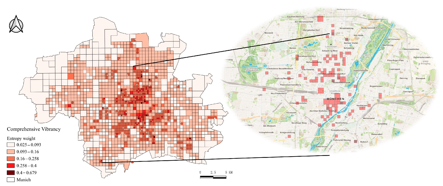
The spatial distribution analysis of comprehensive vibrancy, as shown in Figure 9, reveals a concentration of high-vibrancy areas (represented by deep red grids), primarily in the city center. This observation suggests that the city center plays a critical role in the overall urban vibrancy, with significant contributions from economic, social, cultural, and environmental dimensions. At a more granular scale, these high-vibrancy areas extend concentratedly towards the east and south, following commercial and educational centers within the city center, as well as major roads and metro lines. The southeast direction, in particular, demonstrates exceptionally strong urban vibrancy.
However, the comprehensive vibrancy in the northern and western parts of the city center exhibits relatively sparse distributions compared to the southeast. This pattern implies an imbalance in urban vibrancy across spatial dimensions, which is particularly evident in areas such as Schwanthalerhöhe, Alter Nordfriedhof, Haidhausen, and Oberwiesenfeld. The vibrancy observed in these regions likely originates from the concentration of commercial facilities, cultural institutions, and educational resources that serve as vital sources of urban vibrancy. In summary, Munich demonstrates a spatially uneven urban vibrancy, with a concentration around the city core that extends towards the southeast.
4.1.3. Spatial Correlation in Various Types of Vibrancy
To deeply examine the inherent relationships between economic, social, cultural, and environmental vibrancy as well as with comprehensive vibrancy, this study employs a bivariate Moran’s I spatial autocorrelation analysis. The results are shown in Table 4. It indicates that comprehensive vibrancy has the strongest spatial autocorrelation with social vibrancy, at 0.791, indicating that social vibrancy primarily reflects comprehensive vibrancy, with human activities and aggregation as the core manifestations of urban vibrancy.
Additionally, comprehensive vibrancy exhibits a relatively high spatial autocorrelation with economic vibrancy, at 0.714. In contrast, the spatial autocorrelation between comprehensive and cultural vibrancy is weaker, at only 0.431, suggesting that the spatial distribution of cultural facilities alone cannot well represent comprehensive vibrancy, and cultural vibrancy reflects the static distribution of cultural infrastructure more. Finally, the spatial autocorrelation between comprehensive and environmental vibrancy is negative, at −0.294, denoting discrepancies in the distribution between environmental vibrancy and human activity centers.
Economic vibrancy positively correlates with social vibrancy, with a spatial autocorrelation of 0.642, indicating more vibrant social activity in economically prosperous areas. However, economic vibrancy shows a weaker association with environmental vibrancy, with a spatial autocorrelation of −0.131. Social vibrancy also exhibits positive correlations with cultural and environmental vibrancy, at 0.639 and 0.218, respectively, but the degree is lower than economic vibrancy. Additionally, the spatial autocorrelation between cultural and environmental vibrancy is weak, at 0.167.
In summary, social and economic vibrancy are key determinants of urban comprehensive vibrancy, while cultural and environmental vibrancy demonstrate weaker correlations, with certain discrepancies. These findings provide valuable references for urban planning, while further research is still needed to deeply investigate the inherent drivers and interactions between multiple dimensions of urban vibrancy.
4.2. Comparison of Multiple Models Validation
This study employs spatial regression models based on the global model, taking into account the spatial dependence of various factors in addition to the traditional MLR model. The diagnostic results are shown in Table 5. Both the lag Lagrange multiplier and error Lagrange multiplier show significant values. When both the SLM and SEM diagnostic statistics are simultaneously significant, their corresponding robust statistics are usually examined comprehensively. Among them, the lag robust LM was found to be significant, while the error robust LM was not. Therefore, the SLM should be chosen for regression analysis. However, it should be noted that the Lagrange multiplier test and the selection of the spatial weight matrix are closely related to independent factors. Hence, this study constructs both a spatial lag model (SLM) and a spatial error model (SEM) for regression fitting.
The diagnostic results indicate that the constructed SLM and SEM can better simulate the influence of the built environment on urban vibrancy. Specifically, the adjusted R2 of the SLM and SEM have significantly improved compared to MLR, ranging from 0.363 to 0.452 for different factors, suggesting that the explanatory power was markedly enhanced by incorporating spatial dependence. Meanwhile, the AICc values of the two spatial models are also lower than MLR, reflecting that the fitting effect was improved by considering spatial autocorrelation. The spatial correlation coefficients in the SLM and SEM have passed significance tests, validating the models’ success in capturing the spatial dependence in the data.
This study comprehensively compares the model fitting performances of different factors in global and local models, as shown in Table 6. Overall, the local GWR model demonstrates a better fitting performance than the corresponding global MLR model and SLM. The adjusted R2 and AICc metrics provide validation that incorporating spatial factors significantly improves the explanatory power of the model.
The improved performance of GWR over MLR reflects the influence of geographic spatial autocorrelation on urban vibrancy. Furthermore, the more substantial enhancement of GWR over the SLM indicates that incorporating spatial heterogeneity can further augment the explanatory power of local models. Compared to global models, GWR models exhibit a lower RSS, demonstrating an advantage in fitting outliers and reducing residuals. Additionally, the smaller corrected AICc values of GWR models suggest that they achieve a better balance between the model complexity and goodness-of-fit.
It is noteworthy that although GWR is generally the best-fitting model, the SEM performs better at the global level for certain indicators, particularly in predicting economic vibrancy (Y1) and cultural vibrancy (Y4). This implies that different aspects of urban vibrancy may be influenced by factors operating at different spatial scales, with global factors playing a more significant role in certain types of vibrancy.
In summary, the adoption of local models, particularly the GWR model, effectively captures the inherent spatial complexity and heterogeneity of urban systems, thereby enhancing the accuracy of urban vibrancy modeling. Compared to global models, the GWR model exhibits greater adaptability in capturing local variations in the relationships between the built environment and urban vibrancy across different TAZs within the study area.
4.3. Identification of Influencing Factors
4.3.1. Determining the Influence Factors of Built Environment on Urban Vibrancy
The Geodetector model was employed to examine the impact of various built environment factors on urban vibrancy. The results shown in Table 7 reveal the hierarchical order of factors influencing comprehensive urban vibrancy, which is as follows: The POI density (PD-X2) holds the greatest influence, followed by the building density (BD-X3), intersection density (ID-X4), bus stop density (BS-X8), distance to transit hubs (DTH-X10), road density (RND-X6), population density (RPD-X1), distance to CBD (DCBD-X9), metro station density (MSD-X7), and mixed land use (MUD-X5).
This study demonstrates the significant impact of the built environment on comprehensive urban vibrancy. Notably, the POI density, building density, and road intersection density exert substantial positive effects, with the POI density emerging as the most influential factor, exhibiting a strong positive correlation with urban vibrancy. Abundant and diverse POIs enhance a city’s allure by providing services and amenities catering to inhabitants’ needs. A high building density indicates a greater availability of residential and commercial spaces in central districts, enhancing social resources, services, and the environmental quality. An elevated road intersection density reflects an improved urban connectivity and accessibility, stimulating dynamics and vibrancy through enhanced movement and information exchanges.
Economic vibrancy is primarily influenced by the POI density, followed by the building density and bus station density. A high POI density offers a wide range of consumption options, attracting customers and stimulating economic activity. A high building density provides additional commercial and residential spaces, increasing opportunities for commerce and attracting residents and consumers. An efficient public transportation system facilitates access to consumption locations, reducing costs and promoting economic development.
Social vibrancy is influenced by the distance to the CBD, bus stop density, and POI density. Areas closer to the CBD, with abundant offices, shops, restaurants, and entertainment facilities, exhibit higher social activities due to the influx of commuters and visitors. A high bus stop concentration ensures better public transportation coverage and accessibility. Areas with a high POI density demonstrate an intensified clustering pattern, fostering an increased participation in activities and a heightened social vibrancy.
Cultural vibrancy is primarily related to the distance to transit hubs, building density, and subway station density. Transit hubs attract visitors and often host cultural facilities like museums and theaters, serving as vital venues for cultural exchange. A high building density indicates well-developed infrastructure, attracting cultural activities and diverse facilities. An increased intersection density reflects the road system complexity and connectivity, leading to improved pedestrian traffic and a better flow of information, enhancing cultural vibrancy.
Environmental vibrancy is relatively balanced across built environment factors, with the distances to the CBD and transit hubs having comparatively higher impacts, as areas farther from these locations often exhibit superior environmental quality and serene surroundings.
4.3.2. Exploring the Interactive Factors of Built Environment on Urban Vibrancy
The present study employed interactive analysis to further investigate the synergistic effects of factors on multi-dimensional urban vibrancy, as shown in Table 8. The findings unveiled enhanced bivariate and nonlinear interactions among influencing factors.
This study reveals the presence of nonlinear enhancing interactions between the population density (X1), building density (X3), mixed land use (X5), road network density (X6), metro station density (X7), and bus stop density (X8) on economic vibrancy. This indicates that the combination of the population density with the compactness, connectivity, and public transportation accessibility of the built environment can generate greater economic vibrancy benefits.
The POI density (X2) exhibits bivariate enhancing interactions with the road network density (X6), bus stop density (X8), and distance to transit hubs (X10) on social vibrancy. This suggests that the combination of the facility density and transportation networks facilitates opportunities for social interaction and engagement. The population density (X1) interacts with the building density (X3) and metro station density (X7), while the road intersection density (X4) interacts with the mixed land use (X5), road network density (X6), metro station density (X7), and bus stop density (X8), exhibiting nonlinear enhancing effects on cultural vibrancy. This implies that the confluence of population agglomeration, a compact urban form, and favorable transportation conditions promotes the distribution and utilization of cultural facilities.
The building density (X3) interacts with the mixed land use (X5), metro station density (X7), and bus stop density (X8), while the road intersection density (X4) interacts with the road network density (X6), metro station density (X7), bus stop density (X8), and distance to CBD (X9), exhibiting nonlinear enhancing effects on environmental vibrancy. This highlights the importance of combining compact and diverse land use patterns with accessible transportation conditions for enhancing residents’ quality of life and satisfaction.
The road intersection density (X4) interacts with the mixed land use (X5), road network density (X6), metro station density (X7), and bus stop density (X8), while the mixed land use (X5) interacts with the metro station density (X7), bus stop density (X8), and distance to transit hubs (X10), exhibiting nonlinear enhancing effects on ecological vibrancy. This suggests that the combination of street connectivity, land use diversity, and public transportation accessibility contributes to a greener and more livable urban environment.
Overall, multiple dimensions of urban vibrancy are influenced by the interactive effects of various built environment factors. The road intersection density (X4), road network density (X6), metro station density (X7), and bus stop density (X8) exhibit significant nonlinear enhancing interactions with other factors across multiple dimensions of urban vibrancy, highlighting the crucial role of transportation network connectivity and accessibility in promoting urban vibrancy.
Compared to the influence of single factors, the interactive effects of built environment factors on urban vibrancy are more substantial, reflecting the synergistic effects among different factors. This implies that urban planning and design practices should comprehensively consider the combinations and configurations of multiple built environment factors to maximize urban vibrancy. The research findings also indicate that the impacts of different factor combinations on urban vibrancy exhibit nonlinear relationships, suggesting the existence of threshold effects and optimal combinations rather than simple linear additive effects. It highlights the need to balance the intensities and proportions of different factors and find the optimal equilibrium when optimizing the built environment to enhance urban vibrancy.
5. Discussion
5.1. Theoretical and Practical Implications
The findings of this study have significant theoretical and practical implications for urban planning and management. The differentiated patterns of vibrancy spaces identified in Munich offer valuable insights into the spatial variations of economic, social, cultural, and environmental vibrancy across the city. These insights suggest that city planners and managers should adopt a place-based approach when formulating urban development strategies and allocating public resources, considering the specific vibrancy characteristics and potentials of different areas [43]. This approach can promote a more balanced development of urban vibrancy throughout the city, ensuring that each area’s unique strengths and challenges are addressed effectively.
Moreover, the heterogeneous impact of built environment factors on urban vibrancy provides guidance for urban renewal and spatial optimization [22]. The results indicate that the mechanisms and effects of built environment factors in shaping urban vibrancy vary across different areas, emphasizing the importance of context-specific planning and design. Urban planners and designers should adapt the layout and design of built environment elements to local natural, economic, and social conditions, thereby optimizing the place-specific cultivation of urban vibrancy. This understanding is crucial for informed decision-making in urban regeneration projects and new district development, ensuring that the built environment is tailored to enhance the vibrancy of each area.
5.2. Limitations and Future Research Directions
Despite the significant contributions of this study, several limitations should be acknowledged. Firstly, the use of tweets as a proxy for social vibrancy and cultural POIs as a measure of cultural vibrancy may have shortcomings. The demographic bias of social media users, the uneven spatial distribution of users, and the inability of the cultural POI density to capture intangible cultural aspects could affect the measurement accuracy. Secondly, the assessment of economic vibrancy, although improved by incorporating housing price data, still has limitations. The night-time light data may not accurately reflect the intensity and diversity of economic activities, especially during the daytime. Additionally, the consideration of the quality and productivity of economic activities, rather than just the quantity and density, could further enhance the economic vibrancy assessment by utilizing more detailed data on business types, sizes, and performance. Thirdly, the cross-sectional research design limits the ability to capture the temporal dynamics and evolution of urban vibrancy. Future research could employ time-series analysis to examine the changes in urban vibrancy patterns and their relationship with built environment factors over time, providing a more comprehensive understanding of how urban vibrancy evolves in response to urban development and policy interventions.
To address these limitations and further advance the understanding of urban vibrancy, future research should prioritize the following aspects:
- (1)
- Expanding data sources and analytical approaches. Future research could incorporate more diverse data sources, such as POI utilization rates, social media check-in data, and street view imagery, to enrich the measurement of urban vibrancy. Additionally, the construction of the composite urban vibrancy index could be further refined by exploring alternative weighting schemes, such as principal component analysis or machine learning feature selection methods, and by conducting sensitivity analyses to test the robustness of the results.
- (2)
- Multi-regional comparisons and optimal unit selection. In the future, multi-dimensional comparative empirical research areas can be conducted, and even cities in different countries can be compared to reveal the differences and commonalities of urban vibrancy under different urban planning, cultural contexts, and policy environments. Such cross-city comparative studies are useful for understanding the general patterns and regional characteristics of urban vibrancy. Furthermore, the influence of different scales of urban research units (such as block level, community level, or urban area level) on the research results can be explored, and the scale most suitable for analyzing urban vitality can be determined, ensuring that the modifiable areal unit problem (MAUP) is scientifically feasible [44]. Determining the optimal research unit scale and division method is crucial for understanding and comparing vibrancy between different cities.Novel models and interpretability. Employing novel models and explanatory methods, such as machine learning algorithms like XGBoost, could be valuable in investigating nonlinear relationships between urban vibrancy and the built environment. However, it is crucial to prioritize the interpretability of these models to ensure that the research findings are easily understandable and actionable for urban planners and policymakers, enhancing the practical application value of these outcomes in real-world urban planning and development efforts.
- (3)
- Novel models and interpretability. Employing novel models and explanatory methods, such as machine learning algorithms like XGBoost, could be valuable in investigating nonlinear relationships between urban vibrancy and the built environment. However, it is crucial to prioritize the interpretability of these models to ensure that the research findings are easily understandable and actionable for urban planners and policymakers, enhancing the practical application value of these outcomes in real-world urban planning and development efforts.
6. Conclusions
Urban vibrancy plays a pivotal role in enhancing and sustaining the competitiveness of cities. In light of the challenges faced by many European cities, such as shrinkage, underutilized urban spaces, and insufficiently exploited infrastructure [45], this study explores the intricate relationship between urban vibrancy and the built environment in Munich, Germany, utilizing a multi-source data approach. By integrating multi-source data, a comprehensive assessment framework is constructed to measure various aspects of urban vibrancy. This study reveals the spatial distribution patterns and correlations of different types of urban vibrancy and investigates the multi-dimensional influence of the built environment on urban vibrancy using the 5Ds built environment indicator system.
The findings demonstrate that comprehensive vibrancy in Munich exhibits a pronounced uneven distribution, with higher vibrancy in central and western areas and lower vibrancy in northern and western regions. Highly vibrant areas are concentrated along major roads and metro lines, particularly in commercial and educational centers. The GWR model proves to be the most effective in explaining the relationship between the built environment and vibrancy. Economic, social, and comprehensive vibrancy are significantly influenced by the built environment, with substantial positive effects from the POI density, building density, and road intersection density, while mixed land use shows little impact. Furthermore, interactions among built environment factors, especially the synergistic interactions among the population density, building density, and POI density, generate positive effects on comprehensive vibrancy.
This study contributes to the growing body of research on urban vibrancy and its relationship with the built environment in European cities. The multi-source data approach and comprehensive assessment framework can be applied to other cities, enabling comparative analyses and the identification of context-specific factors influencing urban vibrancy. Future research should focus on expanding the scope of this study to include multiple cities, incorporating additional data sources, and exploring the temporal dynamics of urban vibrancy to gain a more comprehensive understanding of the phenomenon. By leveraging the insights gained from this study, urban planners and policymakers can work towards creating more vibrant, sustainable, and livable cities in Europe and beyond.
Author Contributions
Data curation, C.G. and S.L.; formal analysis, M.S. and C.G.; methodology, M.S. and C.G.; validation, C.G. and X.Z.; visualization, C.G. and S.L.; funding, D.L. writing—original draft, C.G.; writing—review and editing, D.L. All authors have read and agreed to the published version of the manuscript.
Funding
This research was funded by the National Natural Science Foundation of China, grant number 72302119; the China Scholarship Council, grant number 202006560083; and the Jiangsu Social Science Foundation, grant number 23GLC016.
Data Availability Statement
Data are contained within the article.
Acknowledgments
The authors thank Rolf Moeckel from Professorship of Travel Behavior of Technical University of Munich for his comments on this work.
Conflicts of Interest
Author Maopeng Sun was employed by the company Shenzhen Urban Transport Planning Centre. The remaining authors declare that the research was conducted in the absence of any commercial or financial relationships that could be construed as a potential conflict of interest.
References
- Wang, H.; He, Q.; Liu, X.; Zhuang, Y.; Hong, S. Global Urbanization Research from 1991 to 2009: A Systematic Research Review. Landsc. Urban Plan. 2012, 104, 299–309. [Google Scholar] [CrossRef]
- Ameen, R.F.M.; Mourshed, M. Urban Environmental Challenges in Developing Countries—A Stakeholder Perspective. Habitat Int. 2017, 64, 1–10. [Google Scholar] [CrossRef]
- Seeliger, L.; Turok, I. Towards Sustainable Cities: Extending Resilience with Insights from Vulnerability and Transition Theory. Sustainability 2013, 5, 2108–2128. [Google Scholar] [CrossRef]
- Huang, B.; Zhou, Y.; Li, Z.; Song, Y.; Cai, J.; Tu, W. Evaluating and Characterizing Urban Vibrancy Using Spatial Big Data: Shanghai as a Case Study. Environ. Plan. B Urban Anal. City Sci. 2020, 47, 1543–1559. [Google Scholar] [CrossRef]
- Jia, C.; Liu, Y.; Du, Y.; Huang, J.; Fei, T. Evaluation of Urban Vibrancy and Its Relationship with the Economic Landscape: A Case Study of Beijing. ISPRS Int. Geo-Inf. 2021, 10, 72. [Google Scholar] [CrossRef]
- Jacobs, J. The Death and Life of Great American Cities; Reissue edition; Vintage: New York, NY, USA, 1992; ISBN 978-0-679-74195-4. [Google Scholar]
- Landry, C. The Creative City: A Toolkit for Urban Innovators, 1st ed.; Earthscan Publications Ltd.: London, UK, 2000; ISBN 978-1-85383-613-8. [Google Scholar]
- Magurran, A. Ecological Diversity and Its Measurement, 1st ed.; Croom Helm: London, UK, 1988; ISBN 978-0-7099-3539-1. [Google Scholar]
- Wang, S.; Wang, J.; Li, W.; Fan, J.; Liu, M. Revealing the Influence Mechanism of Urban Built Environment on Online Car-Hailing Travel Considering Orientation Entropy of Street Network. Discret. Dyn. Nat. Soc. 2022, 2022, 3888800. [Google Scholar] [CrossRef]
- Kang, C.; Fan, D.; Jiao, H. Validating Activity, Time, and Space Diversity as Essential Components of Urban Vitality. Environ. Plan. B-Urban Anal. City Sci. 2021, 48, 1180–1197. [Google Scholar] [CrossRef]
- Wu, J.; Wang, B.; Wang, R.; Ta, N.; Chai, Y. Active Travel and the Built Environment: A Theoretical Model and Multidimensional Evidence. Transport. Res. Part D-Transport. Environ. 2021, 100, 103029. [Google Scholar] [CrossRef]
- Gao, C.; Lai, X.; Li, S.; Cui, Z.; Long, Z. Bibliometric Insights into the Implications of Urban Built Environment on Travel Behavior. ISPRS Int. J. Geo-Inf. 2023, 12, 453. [Google Scholar] [CrossRef]
- Gómez-Varo, I.; Delclòs-Alió, X.; Miralles-Guasch, C. Jane Jacobs Reloaded: A Contemporary Operationalization of Urban Vitality in a District in Barcelona. Cities 2022, 123, 103565. [Google Scholar] [CrossRef]
- Cao, X.; Mokhtarian, P.L.; Handy, S.L. Do Changes in Neighborhood Characteristics Lead to Changes in Travel Behavior? A Structural Equations Modeling Approach. Transportation 2007, 34, 535–556. [Google Scholar] [CrossRef]
- Cervero, R.; Kockelman, K. Travel Demand and the 3Ds: Density, Diversity, and Design. Transp. Res. Part D Transp. Environ. 1997, 2, 199–219. [Google Scholar] [CrossRef]
- Ewing, R.; Cervero, R. Travel and the Built Environment: A Meta-Analysis. J. Am. Plan. Assoc. 2010, 76, 265–294. [Google Scholar] [CrossRef]
- Chen, L.; Lu, Y.; Ye, Y.; Xiao, Y.; Yang, L. Examining the Association between the Built Environment and Pedestrian Volume Using Street View Images. Cities 2022, 127, 103734. [Google Scholar] [CrossRef]
- Sung, H.; Lee, S. Residential Built Environment and Walking Activity: Empirical Evidence of Jane Jacobs’ Urban Vitality. Transp. Res. Part D Transp. Environ. 2015, 41, 318–329. [Google Scholar] [CrossRef]
- Jiang, H.; Dong, L.; Qiu, B. How Are Macro-Scale and Micro-Scale Built Environments Associated with Running Activity? The Application of Strava Data and Deep Learning in Inner London. ISPRS Int. J. Geo-Inf. 2022, 11, 504. [Google Scholar] [CrossRef]
- Ma, D.; Osaragi, T.; Oki, T.; Jiang, B. Exploring the Heterogeneity of Human Urban Movements Using Geo-Tagged Tweets. Int. J. Geogr. Inf. Sci. 2020, 34, 2475–2496. [Google Scholar] [CrossRef]
- Lin, C.; Liu, G.; Müller, D.B. Characterizing the Role of Built Environment Stocks in Human Development and Emission Growth. Resour. Conserv. Recycl. 2017, 123, 67–72. [Google Scholar] [CrossRef]
- Yang, X.; Zhao, Z.; Shi, C.; Luo, L.; Tu, W. The Dynamic Heterogeneous Relationship between Urban Population Distribution and Built Environment in Xi’an, China: A Case Study. Remote Sens. 2023, 15, 2257. [Google Scholar] [CrossRef]
- Cheng, L.; Shi, K.; De Vos, J.; Cao, M.; Witlox, F. Examining the Spatially Heterogeneous Effects of the Built Environment on Walking among Older Adults. Transp. Policy 2021, 100, 21–30. [Google Scholar] [CrossRef]
- Chen, L.; Zhao, L.; Xiao, Y.; Lu, Y. Investigating the Spatiotemporal Pattern between the Built Environment and Urban Vibrancy Using Big Data in Shenzhen, China. Comput. Environ. Urban Syst. 2022, 95, 101827. [Google Scholar] [CrossRef]
- Li, J.; Lo, K.; Zhang, P.; Guo, M. Relationship between Built Environment, Socio-Economic Factors and Carbon Emissions from Shopping Trip in Shenyang City, China. Chin. Geogr. Sci. 2017, 27, 722–734. [Google Scholar] [CrossRef]
- Shi, Y.; Zheng, J.; Pei, X. Measurement Method and Influencing Mechanism of Urban Subdistrict Vitality in Shanghai Based on Multisource Data. Remote Sens. 2023, 15, 932. [Google Scholar] [CrossRef]
- Mouratidis, K. Urban Planning and Quality of Life: A Review of Pathways Linking the Built Environment to Subjective Well-Being. Cities 2021, 115, 103229. [Google Scholar] [CrossRef]
- Alavipanah, S.; Wegmann, M.; Qureshi, S.; Weng, Q.; Koellner, T. The Role of Vegetation in Mitigating Urban Land Surface Temperatures: A Case Study of Munich, Germany during the Warm Season. Sustainability 2015, 7, 4689–4706. [Google Scholar] [CrossRef]
- Montgomery, J. Making a City: Urbanity, Vitality and Urban Design. J. Urban Des. 1998, 3, 93–116. [Google Scholar] [CrossRef]
- Sung, H.; Lee, S.; Cheon, S. Operationalizing Jane Jacobs’s Urban Design Theory: Empirical Verification from the Great City of Seoul, Korea. J. Plan. Educ. Res. 2015, 35, 117–130. [Google Scholar] [CrossRef]
- Jones, C.; Newsome, D. Perth (Australia) as One of the World’s Most Liveable Cities: A Perspective on Society, Sustainability and Environment. Int. J. Tour. Cities 2015, 1, 18–35. [Google Scholar] [CrossRef]
- Bennett, M.M.; Smith, L.C. Advances in Using Multitemporal Night-Time Lights Satellite Imagery to Detect, Estimate, and Monitor Socioeconomic Dynamics. Remote Sens. Environ. 2017, 192, 176–197. [Google Scholar] [CrossRef]
- Wu, C.; Ye, X.; Ren, F.; Wan, Y.; Ning, P.; Du, Q. Spatial and Social Media Data Analytics of Housing Prices in Shenzhen, China. PLoS ONE 2016, 11, e0164553. [Google Scholar] [CrossRef]
- Yue, Y.; Zhuang, Y.; Yeh, A.G.; Xie, J.Y.; Ma, C.L.; Li, Q.Q. Measurements of POI-Based Mixed Use and Their Relationships with Neighbourhood Vibrancy. Int. J. Geogr. Inf. Sci. 2017, 31, 658–675. [Google Scholar] [CrossRef]
- Kang, C.-D. Effects of Spatial Access to Neighborhood Land-Use Density on Housing Prices: Evidence from a Multilevel Hedonic Analysis in Seoul, South Korea. Environ. Plan. B-Urban Anal. City Sci. 2019, 46, 603–625. [Google Scholar] [CrossRef]
- Zhou, Y.; He, X.; Zikirya, B. Boba Shop, Coffee Shop, and Urban Vitality and Development—A Spatial Association and Temporal Analysis of Major Cities in China from the Standpoint of Nighttime Light. Remote Sens. 2023, 15, 903. [Google Scholar] [CrossRef]
- Huang, H.; Yao, X.A.; Krisp, J.M.; Jiang, B. Analytics of Location-Based Big Data for Smart Cities: Opportunities, Challenges, and Future Directions. Comput. Environ. Urban Syst. 2021, 90, 101712. [Google Scholar] [CrossRef]
- Chen, Y.; Yu, B.; Shu, B.; Yang, L.; Wang, R. Exploring the Spatiotemporal Patterns and Correlates of Urban Vitality: Temporal and Spatial Heterogeneity. Sustain. Cities Soc. 2023, 91, 104440. [Google Scholar] [CrossRef]
- Anselin, L. Spatial Econometrics: Methods and Models; Springer Science & Business Media: Berlin/Heidelberg, Germany, 1988; ISBN 978-90-247-3735-2. [Google Scholar]
- Anselin, L. Local Indicators of Spatial Association—LISA. Geogr. Anal. 1995, 27, 93–115. [Google Scholar] [CrossRef]
- Wang, J.; Li, X.; Christakos, G.; Liao, Y.; Zhang, T.; Gu, X.; Zheng, X. Geographical Detectors-Based Health Risk Assessment and Its Application in the Neural Tube Defects Study of the Heshun Region, China. Int. J. Geogr. Inf. Sci. 2010, 24, 107–127. [Google Scholar] [CrossRef]
- Wang, J.-F.; Zhang, T.-L.; Fu, B.-J. A Measure of Spatial Stratified Heterogeneity. Ecol. Indic. 2016, 67, 250–256. [Google Scholar] [CrossRef]
- Meng, Y.; Xing, H. Exploring the Relationship between Landscape Characteristics and Urban Vibrancy: A Case Study Using Morphology and Review Data. Cities 2019, 95, 102389. [Google Scholar] [CrossRef]
- Gao, F.; Li, S.; Tan, Z.; Wu, Z.; Zhang, X.; Huang, G.; Huang, Z. Understanding the Modifiable Areal Unit Problem in Dockless Bike Sharing Usage and Exploring the Interactive Effects of Built Environment Factors. Int. J. Geogr. Inf. Sci. 2021, 35, 1905–1925. [Google Scholar] [CrossRef]
- Wolff, M.; Wiechmann, T. Urban Growth and Decline: Europe’s Shrinking Cities in a Comparative Perspective 1990–2010. Eur. Urban Reg. Stud. 2018, 25, 122–139. [Google Scholar] [CrossRef]
Figure 1.
Study area of Munich, Germany.
Figure 2.
The workflow of this study.
Figure 3.
Various types of urban vibrancy.
Figure 4.
Bivariate spatial autocorrelation of the LISA analysis.

Figure 5.
The spatial distribution of economic vibrancy in Munich.
Figure 6.
The spatial distribution of social vibrancy in Munich.
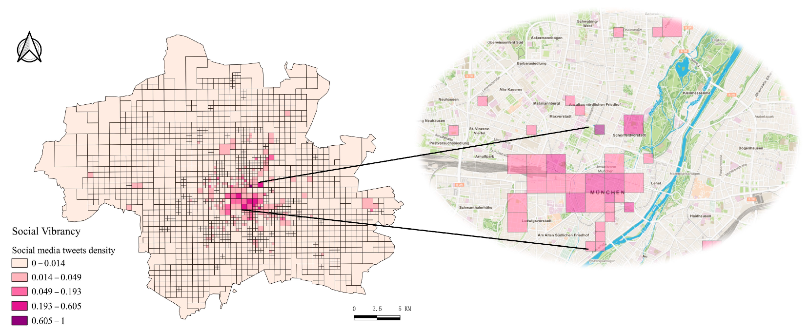
Figure 7.
The spatial distribution of cultural vibrancy in Munich.
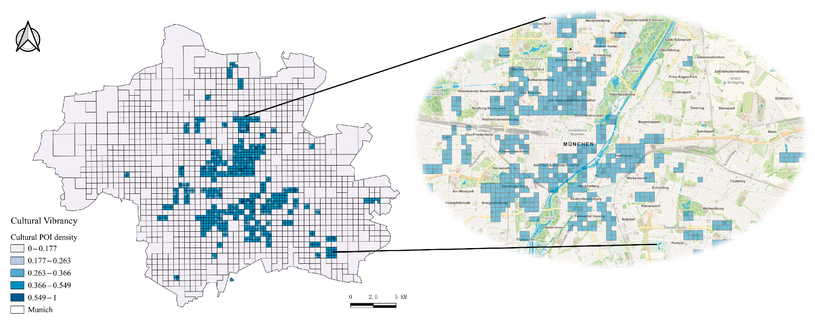
Figure 8.
The spatial distribution of environmental vibrancy in Munich.
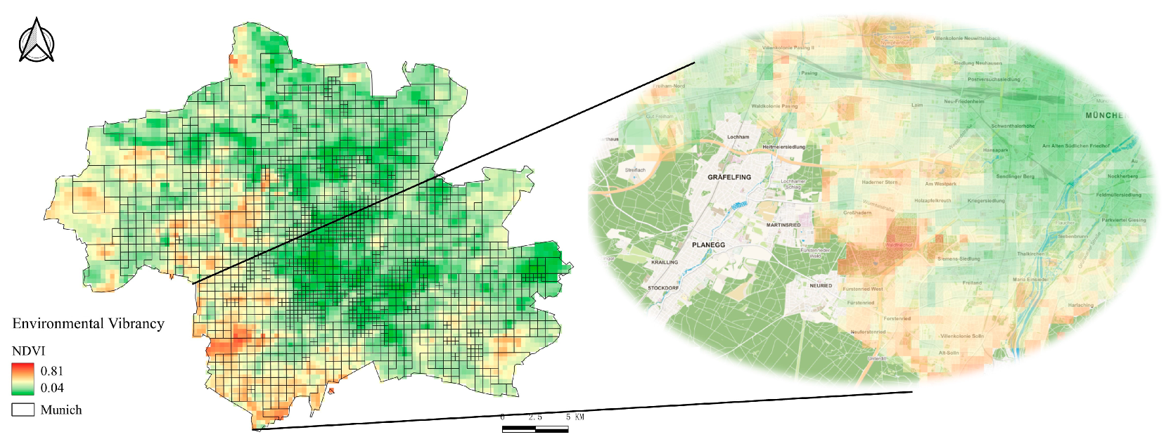
Figure 9.
The spatial distribution of comprehensive vibrancy in Munich.

Table 1.
Description of various urban vibrancy datasets.
| Data | Source | Numbers and Type | Time Period | Spatial Resolution |
|---|---|---|---|---|
| Night-time light | Annual composite imagery of night-time light from https://ngdc.noaa.gov, accessed on 22 June 2023 | Raster tiff | 2019 | 500 m |
| Housing price | Munich average house price from https://www.opengov-muenchen.de, accessed on 22 June 2023 | 974,393 vector polygons | 2018 | / |
| Social media tweets | Geotagged tweets from https://developer.twitter.com/en/docs/twitter-api, accessed on 22 June 2023 | 1,176,798 vector points | 2018–2019 | / |
| Cultural POIs | Locations of cultural venues from https://www.openstreetmap.org/, accessed on 22 June 2023 | 163,505 vector points | 2019 | / |
| NDVI value | Sentinel-2 satellite imagery from https://sentinels.copernicus.eu/web/sentinel/sentinel-2, accessed on 22 June 2023 | Raster tiff | June 2020 | 10 m |
Table 2.
Overview of factors and descriptive analysis.
| No. | Factors | Abb. | Min | Mean | Max | Std. | VIF |
|---|---|---|---|---|---|---|---|
| 1 | Night-time light | EI-Y1 | 0 | 2078 | 7,315,148 | 298,403.9 | / |
| Housing price | 9.3 | 16.80 | 42.70 | 3.70 | / | ||
| 2 | Social media tweet density (million·km−2) | SI-Y2 | 0 | 9633.9 | 1312.1 | 47,983.9 | / |
| 3 | Cultural POI density (million·km−2) | CI-Y3 | 0 | 53.70 | 1275 | 100.50 | / |
| 4 | NDVI | VI-Y4 | 0 | 0.41 | 0.81 | 0.23 | / |
| 5 | Comprehensive vibrancy | UI-Y5 | 0.025 | 0.349 | 0.679 | 0.190 | / |
| 6 | Population density (million·km−2) | RPD-X1 | 0 | 9031.40 | 34,300 | 7958 | 1.254 |
| 7 | POI density (million·km−2) | PD-X2 | 0 | 2204.70 | 30,750 | 2981.10 | 1.635 |
| 8 | Building density (million·km−2) | BD-X3 | 0 | 270 | 3754 | 285.6 | 2.187 |
| 9 | Intersection density | ID-X4 | 0 | 3194.90 | 72,500 | 5896.90 | 1.981 |
| 10 | Mixed land use | MUD-X5 | 0 | 0.11 | 0.93 | 0.14 | 1.473 |
| 11 | Road network density | RND-X6 | 55,786.6 | 36,834.6 | 93,112.8 | 139,778 | 1.842 |
| 12 | Metro station density | MSD-X7 | 0 | 8.60 | 500 | 40.40 | 2.197 |
| 13 | Bus stop density | BS-X8 | 0 | 104.40 | 2000 | 175.30 | 2.214 |
| 14 | Distance to the CBD (km) | DCBD-X9 | 0.27 | 6.30 | 15.90 | 2.90 | 1.127 |
| 15 | Distance to transit hubs (km) | DTH-X10 | 0.26 | 6.30 | 15.00 | 2.90 | 1.564 |
Table 3.
Interactive types between two factors.
| Criterion | Interaction Types |
|---|---|
| q(X1∩X2) < Min(q(X1), q(X2)) | Nonlinear, weakens |
| Min(q(X1), q(X2)) < q(X1∩X2) < Max(q(X1), q(X2)) | Univariate, weakens |
| q(X1∩X2) > Max(q(X1), q(X2)) | Bivariate, enhances |
| q(X1∩X2) = q(X1) + q(X2) | Independent |
| q(X1∩X2) > q(X1) + q(X2) | Nonlinear, enhances |
Table 4.
Moran’s I spatial correlation in various types of vibrancy.
| Factors | Moran’s I | |
|---|---|---|
| Comprehensive vibrancy (Y5) | Economic vibrancy (Y1) | 0.714 |
| Comprehensive vibrancy (Y5) | Social vibrancy (Y2) | 0.791 |
| Comprehensive vibrancy (Y5) | Cultural vibrancy (Y3) | 0.431 |
| Comprehensive vibrancy (Y5) | Environmental vibrancy (Y4) | −0.294 |
| Economic vibrancy (Y1) | Social vibrancy (Y2) | 0.642 |
| Economic vibrancy (Y1) | Cultural vibrancy (Y3) | 0.352 |
| Economic vibrancy (Y1) | Environmental vibrancy (Y4) | −0.131 |
| Social vibrancy (Y2) | Cultural vibrancy (Y3) | 0.639 |
| Social vibrancy (Y2) | Environmental vibrancy (Y4) | 0.218 |
| Cultural vibrancy (Y3) | Environmental vibrancy (Y4) | 0.167 |
Table 5.
Diagnostic results of spatial dependence based on MLR.
| Test Type | Standardized Value of Test Statistic | Test Statistic | p-Value |
|---|---|---|---|
| Moran’s I—error | 0.0923 | 3.123 | 0.00179 |
| Lagrange multiplier—lag | 1 | 11.1597 | 0.00084 |
| Robust LM—lag | 1 | 8.0495 | 0.00455 |
| Lagrange multiplier—error | 1 | 5.7283 | 0.01669 |
| Robust LM—error | 1 | 2.6181 | 0.10565 |
| Lagrange multiplier—SARMA | 2 | 13.7778 | 0.00102 |
Table 6.
Comparison of model fitting between global and local models.
| Global Models | Adj. R2 | RSS | AICc | Local Models | Adj. R2 | RSS | AICc |
|---|---|---|---|---|---|---|---|
| MLR(Y1) | 0.288 | 71.691 | −127.382 | GWR(Y1) | 0.505 | 99.945 | 501.959 |
| SLM(Y1) | 0.438 | 86.981 | −155.962 | ||||
| SEM(Y1) | 0.452 | 88.490 | −160.98 | ||||
| MLR(Y2) | 0.370 | 98.534 | −181.068 | GWR(Y2) | 0.592 | 82.506 | 473.456 |
| SLM(Y2) | 0.431 | 99.471 | −180.941 | ||||
| SEM(Y2) | 0.447 | 101.039 | −186.078 | ||||
| MLR(Y3) | 0.310 | 94.805 | −173.611 | GWR(Y3) | 0.520 | 96.899 | 499.738 |
| SLM(Y3) | 0.380 | 100.03 | −182.061 | ||||
| SEM(Y3) | 0.273 | 83.38 | −150.76 | ||||
| MLR(Y4) | 0.314 | 89.783 | −163.566 | GWR(Y4) | 0.574 | 86.082 | 475.654 |
| SLM(Y4) | 0.382 | 94.885 | −171.770 | ||||
| SEM(Y4) | 0.368 | 92.923 | −169.847 | ||||
| MLR(Y5) | 0.614 | 77.958 | 455.164 | GWR(Y5) | 0.601 | 80.694 | 476.205 |
| SLM(Y5) | 0.603 | 80.123 | 476.595 | ||||
| SEM(Y5) | 0.640 | 72.698 | 455.564 |
Table 7.
The detection results of built environmental factors on urban vibrancy.
| Detection Factors | Y1 | Y2 | Y3 | Y4 | Y5 |
|---|---|---|---|---|---|
| RPD-X1 | 0.101 ** | 0.128 ** | 0.194 ** | 0.048 ** | 0.131 ** |
| PD-X2 | 0.414 ** | 0.164 ** | 0.157 ** | 0.106 ** | 0.593 ** |
| BD-X3 | 0.393 ** | 0.116 ** | 0.290 ** | 0.169 * | 0.443 ** |
| ID-X4 | 0.212 ** | 0.196 * | 0.112 ** | 0.143 * | 0.199 ** |
| MUD-X5 | 0.049 ** | 0.161 ** | 0.124 ** | 0.121 ** | 0.057 ** |
| RND-X6 | 0.120 ** | 0.139 ** | 0.127 ** | 0.091 * | 0.141 ** |
| MSD-X7 | 0.043 * | 0.131 ** | 0.264 ** | 0.109 * | 0.069 * |
| BS-X8 | 0.249 ** | 0.167 * | 0.101 ** | 0.175 ** | 0.187 ** |
| DCBD-X9 | 0.101 ** | 0.169 ** | 0.171 ** | 0.198 * | 0.109 ** |
| DTH-X10 | 0.099 ** | 0.127 ** | 0.306 ** | 0.189 * | 0.149 ** |
* and ** indicate that the variables pass the significance tests of 0.1 and 0.05, respectively.
Table 8.
The influencing results of interaction factors on urban vibrancy.
| A∩B | Y1 | Y2 | Y3 | Y4 | Y5 | A∩B | Y1 | Y2 | Y3 | Y4 | Y5 |
|---|---|---|---|---|---|---|---|---|---|---|---|
| X1∩X2 | 0.351 | 0.201 | 0.171 | 0.094 | 0.511 | X3∩X10 | 0.354 | 0.115 | 0.251 | 0.151 | 0.401 |
| X1∩X3 | 0.399 * | 0.186 | 0.221 * | 0.152 | 0.434 | X4∩X5 | 0.201 | 0.11 | 0.151 * | 0.123 | 0.220 * |
| X1∩X4 | 0.211 | 0.206 | 0.131 | 0.141 | 0.199 | X4∩X6 | 0.221 * | 0.192 * | 0.184 * | 0.146 * | 0.241 * |
| X1∩X5 | 0.129 * | 0.154 | 0.145 | 0.120 | 0.131 | X4∩X7 | 0.232 * | 0.221 * | 0.261 * | 0.169 * | 0.254 * |
| X1∩X6 | 0.154 * | 0.173 | 0.164 | 0.099 | 0.186 * | X4∩X8 | 0.264 * | 0.239 * | 0.191 * | 0.171 * | 0.271 * |
| X1∩X7 | 0.121 * | 0.164 | 0.21 * | 0.108 | 0.141 | X4∩X9 | 0.191 | 0.201 * | 0.224 * | 0.152 * | 0.197 |
| X1∩X8 | 0.202 * | 0.182 | 0.152 | 0.171 | 0.181 * | X4∩X10 | 0.194 | 0.216 * | 0.301 | 0.133 | 0.199 |
| X1∩X9 | 0.132 | 0.186 | 0.174 | 0.192 | 0.156 | X4∩X6 | 0.119 | 0.151 | 0.117 | 0.111 | 0.127 |
| X1∩X10 | 0.131 | 0.168 | 0.251 | 0.142 | 0.147 | X5∩X7 | 0.131 * | 0.161 | 0.241 * | 0.122 * | 0.171 * |
| X2∩X3 | 0.401 * | 0.171 | 0.22 | 0.162 * | 0.516 | X5∩X8 | 0.161 * | 0.171 * | 0.154 * | 0.131 * | 0.179 * |
| X2∩X4 | 0.311 | 0.224 * | 0.134 | 0.151 | 0.309 | X5∩X9 | 0.112 | 0.161 | 0.171 | 0.114 | 0.15 |
| X2∩X5 | 0.303 | 0.141 | 0.156 | 0.125 | 0.297 | X5∩X10 | 0.141 | 0.159 | 0.289 | 0.148 | 0.154 * |
| X2∩X6 | 0.334 | 0.221 * | 0.167 | 0.095 | 0.364 | X6∩X7 | 0.161 * | 0.139 * | 0.215 * | 0.112 * | 0.211 * |
| X2∩X7 | 0.326 | 0.111 | 0.211 | 0.11 | 0.336 | X6∩X8 | 0.196 * | 0.201 * | 0.171 * | 0.144 | 0.221 * |
| X2∩X8 | 0.368 | 0.214 * | 0.157 | 0.182 | 0.397 | X6∩X9 | 0.153 * | 0.184 * | 0.191 * | 0.161 * | 0.204 * |
| X2∩X9 | 0.354 | 0.134 | 0.176 | 0.201 | 0.356 | X6∩X10 | 0.141 | 0.171 * | 0.294 | 0.177 * | 0.149 |
| X2∩X10 | 0.356 | 0.19 * | 0.234 | 0.196 | 0.374 | X7∩X8 | 0.211 | 0.147 * | 0.273 * | 0.197 * | 0.265 * |
| X3∩X4 | 0.302 | 0.201 | 0.201 | 0.156 | 0.322 | X7∩X9 | 0.171 * | 0.149 | 0.214 | 0.144 | 0.244 * |
| X3∩X5 | 0.297 | 0.146 | 0.214 * | 0.171 * | 0.306 | X7∩X10 | 0.129 | 0.209 * | 0.317 * | 0.167 * | 0.106 |
| X3∩X6 | 0.322 | 0.131 | 0.210 | 0.146 | 0.374 | X8∩X9 | 0.071 | 0.241 * | 0.161 | 0.172 | 0.104 |
| X3∩X7 | 0.322 | 0.191 * | 0.251 * | 0.157 * | 0.347 | X8∩X10 | 0.141 | 0.234 * | 0.331 * | 0.221 * | 0.159 |
| X3∩X8 | 0.356 | 0.167 * | 0.201 | 0.221 * | 0.403 | X9∩X10 | 0.131 | 0.112 | 0.302 | 0.141 | 0.148 |
| X3∩X9 | 0.346 | 0.114 | 0.197 | 0.149 | 0.361 |
* Indicates nonlinear enhancement; no mark indicates bivariate enhancement.
Disclaimer/Publisher’s Note: The statements, opinions and data contained in all publications are solely those of the individual author(s) and contributor(s) and not of MDPI and/or the editor(s). MDPI and/or the editor(s) disclaim responsibility for any injury to people or property resulting from any ideas, methods, instructions or products referred to in the content. |
© 2024 by the authors. Licensee MDPI, Basel, Switzerland. This article is an open access article distributed under the terms and conditions of the Creative Commons Attribution (CC BY) license (https://creativecommons.org/licenses/by/4.0/).
Share and Cite
MDPI and ACS Style
Gao, C.; Li, S.; Sun, M.; Zhao, X.; Liu, D. Exploring the Relationship between Urban Vibrancy and Built Environment Using Multi-Source Data: Case Study in Munich. Remote Sens. 2024, 16, 1107. https://doi.org/10.3390/rs16061107
AMA Style
Gao C, Li S, Sun M, Zhao X, Liu D. Exploring the Relationship between Urban Vibrancy and Built Environment Using Multi-Source Data: Case Study in Munich. Remote Sensing. 2024; 16(6):1107. https://doi.org/10.3390/rs16061107
Chicago/Turabian StyleGao, Chao, Shasha Li, Maopeng Sun, Xiyang Zhao, and Dewen Liu. 2024. "Exploring the Relationship between Urban Vibrancy and Built Environment Using Multi-Source Data: Case Study in Munich" Remote Sensing 16, no. 6: 1107. https://doi.org/10.3390/rs16061107
Note that from the first issue of 2016, this journal uses article numbers instead of page numbers. See further details here.