PrISM at Operational Scale: Monitoring Irrigation District Water Use during Droughts

Abstract

Efficient water management strategies are of utmost importance in drought-prone regions, given the fundamental role irrigation plays in avoiding yield losses and food shortages. Traditional methodologies for estimating irrigation amounts face limitations in terms of overall precision and operational scalability. This study proposes to estimate irrigation amounts from soil moisture (SM) data by adapting the PrISM (Precipitation Inferred from Soil Moisture) methodology. The PrISM assimilates SM into a simple Antecedent Precipitation Index (API) model using a particle filter approach, which allows the creation and estimation of irrigation events. The methodology is applied in a semi-arid region in the Ebro basin, located in the north-east of Spain (Catalonia), from 2016 to 2023. Multi-year drought, which started in 2020, particularly affected the region starting from the spring of 2023, which led to significant reductions in irrigation district water allocations in some of the areas of the region. This study demonstrates that the PrISM approach can correctly identify areas where water restrictions were adopted in 2023, and monitor the water usage with good performances and reliable results. When compared with in situ data for 8 consecutive years, PrISM showed a significant person’s correlation between $0.58$ and $0.76$ and a cumulative weekly root mean squared error (rmse) between 7 and 11 mm. Additionally, PrISM was applied to three irrigation districts with different levels of modernization, due to the different predominant irrigation systems: flood, sprinkler, and drip. This analysis underlined the strengths and limitations of PrISM depending on the irrigation techniques monitored. PrISM has good performances in areas irrigated by sprinkler and flood systems, while difficulties are present over drip irrigated areas, where the very localized and limited irrigation amounts could not be detected from $SM$ observations.

1. Introduction

Droughts are a recurrent and intensifying phenomenon on a global scale, with a strong impact on the agricultural sector [1,2,3,4,5]. The Working Group I for the IPCC report of 2021 [6,7] concluded with high confidence that the likelihood of drought is projected to increase in many regions over the 21st century even with strong climate change mitigation, and more severely in the absence of this.

Spain was the European country most affected by the long drought period during the spring of 2023 [8], and it is one of the most vulnerable countries in terms of future water availability [9]. Almost no meaningful rainfall event has happened in cropland areas in the first 5 months of 2023: recorded precipitation has been the lowest since 1991 and temperatures and solar radiation levels have been strongly above the long-term average (LTA) [10,11]. Following the large drought event, which intensified in 2023 but started already in 2020, many water policymakers and irrigation district managers were forced to impose severe water restrictions on water allocations, reducing water amounts by 20 to 70% depending on the irrigation district and watershed [12]. The scarcity of freshwater resources immediately affects the agricultural sector, which is the primary driver of freshwater use. Irrigation uses 70% of the total freshwater at the global scale [13,14,15], and was estimated to be around 65% in 2019 for Spain [13,16]. Monitoring the spatial and temporal distribution of irrigation is therefore of utmost importance to further optimize freshwater use and avoid great yield losses. Operational methodologies that produce precise and timely information are still lacking on both a global and local scale, and it is key to supporting water management decisions [17].

Remote sensing offers large amounts of continuous and uniform data at a global scale of the crop and soil water status. For this reason, there is an increasing interest in exploiting these types of datasets to retrieve information on irrigation practices. First efforts focused on mapping irrigation areas, progressing from global [18,19,20] to regional [21,22,23] and field scale [24]. More recently efforts have been made toward developing remote-sensing techniques for irrigation estimation. As described by Kragh et al. [25], current approaches can be divided into 3 distinct groups, based on the methodology used to estimate irrigation with remote-sensing data.

The first group is based on directly retrieving irrigation estimates from remote-sensing data using soil moisture ($SM$), vegetation indices, or actual evapotranspiration ($ET$) as a proxy. Brocca et al. [26] proposed directly using $SM$ observations to retrieve irrigation by inverting the water balance equation. Dari et al. [27] applied and validated this SM-based inversion approach, called SM2RAIN, in a semi-arid region in Catalunya, and successively improved the process by integrating actual evapotranspiration ($ET$) into the water balance equation [28]. Nevertheless, the simple inversion technique proposed by the SM2RAIN was shown to be sensitive to uncertainties contained in the few calibrated parameters of this approach, and it showed difficulties in estimating irrigation during rainier seasons and in discriminating between precipitation and irrigation amounts [26,29]. Other approaches showed promising results by using remotely sensed vegetation indexes in the FAO-56 model adapted for a Remote Sensing-based Soil Water Balance [30] or the SAMIR model ([31,32]). Wei et al. [33] used instead remote-sensing vegetation indexes and meteorological variables to train a machine learning model to predict irrigation amounts.

The second group of approaches estimates irrigation amounts from differences between observed and modeled hydrological variables, such as surface SM [34,35], actual ET [36,37], or root-zone SM [38]. Modeled variables are often produced from Hydrological or Land Surface Models (LSM) that do not have an irrigation scheme implemented. Irrigation is then estimated as the difference between real observations and modeled variables. A drawback of this approach is the assumption that the difference between modeled and observed hydrological variables is exclusively related to irrigation: modeling errors, errors in the observations, or rescaling errors between the two independent inputs could mask the real effect of irrigation on these variables. Similarly to these approaches, Brombacher et al. [37] proposed retrieving irrigation by calculating the difference between actual ET from irrigated fields and actual ET from nearby hydrological similar natural areas, instead of modeled ET. This approach overcomes the difficulties in harmonizing modeled and observed hydrological variables, but it is only effective in case enough hydrological similar pixels from natural areas are available in the study area.

The third group of approaches estimates irrigation amounts directly by assimilating $SM$ observations into Land Surface Models and simulating irrigation events with this information [39,40,41]. Even if quite robust and accurate, LSMs often require many inputs to completely simulate the plant and soil at each step, and extensive calibration, reducing the possibility of large-scale operationalization of the approach. LSM models also require computationally expensive operations to produce accurate simulations, which further limits their large-scale applicability for near real-time detection of irrigation amounts.

In this framework, PrISM (Precipitation Inferred Soil Moisture) is proposed as a hybrid method between the first and third groups. This methodology employs a data assimilation scheme, similar to LSM models, to incorporate $SM$ observations into the Antecedent Precipitation Index (API) model. The data assimilation ensures the same robustness of the methods belonging to the third group while ensuring lightweight computations given the use of the API model, which is a semi-empirical integration of the water-balance equation [42]. The use of the API can be related to the approaches of the first group, which have a similar order of complexity and the same small number of parameters.

The main objective of this paper is to investigate the performance of a remote-sensing algorithm for irrigation estimation in the context of water scarcity. Previous studies have always validated irrigation products against in situ data collected during years where no restrictions were implemented and plants were irrigated to their full potential. In this study, we focus on understanding the sensitivity of remote-sensing approaches in detecting and estimating large reductions in water allocations, which often occur as emergency measures during large drought periods. These restrictions are expected to be increasingly more frequent, especially given the future scenario of higher temperatures and lower precipitation during the dry season, as forecasted in particular for the Mediterranean region. For this reason, it is quite important to verify the capability to map and estimate large changes in irrigation amounts allocated at the district level.

2. Materials and Methods

2.1. Study Area

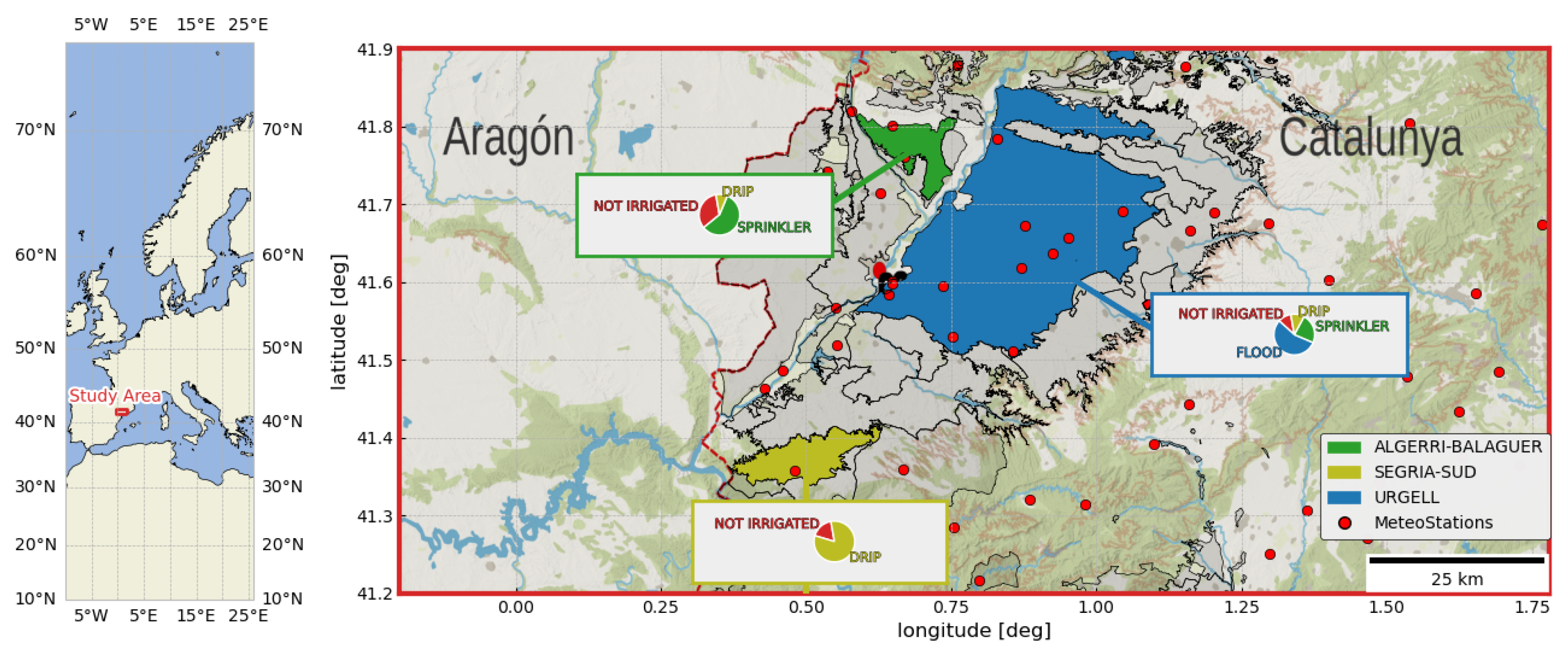
The study area is located in the province of Lleida, in the north-east of Spain. The area is characterized by a Mediterranean semi-arid climate, with hot and dry summers: the total average seasonal precipitation between June and September is around 50 mm, with an average temperature of 24 °C degrees and several days with peaks above 40 °C degrees. The average annual precipitation is between 300 and 400 mm, with most of the rainfall occurring in autumn and spring [43]. The area is mostly flat and characterized by high agricultural activity, with an elevation which is always between 350 m and 150 m and a rather homogeneous soil texture, with around $50\%$ sand, $15\%$ clay, and $35\%$ silt (https://esdac.jrc.ec.europa.eu/resource-type/soil-data-maps, accessed on 3 March 2024). Most of the fields are heavily irrigated in spring and summer through a large open canal system that conveys water from the Pyrenees. The main crops present in the area are winter cereals, maize, fruit trees, and vegetables. Three different irrigation districts are selected for this study: Canals d’Urgell, Algerri-Balaguer, and Segria Sud. The three districts were selected because of their very different irrigation practices, with flood irrigation being the most common system employed in Canals d’Urgell, the sprinkler irrigation being mostly adopted in Algerri-Balaguer, and drip irrigation in Segria Sud. Figure 1 depicts the study area with the three irrigation districts and the distribution of the different irrigation systems according to data extracted from SIGPAC (Sistema de Información Geográfica de Parcelas Agrícolas) (https://agricultura.gencat.cat/ca/ambits/desenvolupament-rural/sigpac/mapa-cultius/, accessed on 15 January 2024) of 2021. SIGPAC is an administrative dataset that collects multiple information at the field level with regards to field shape and area, type of crops cultivated, irrigation system (if present), and irrigation coefficients.

The three irrigation districts show multiple differences, not only in terms of irrigation systems but also in the amount and frequency of irrigation water applied and the types of crops grown. The Canals d’Urgell district is the largest one, with a total area of around 887 km² and a total irrigated area of around 650 km². The irrigated water is supplied by two canals, called “main” and “auxiliary”, which serve the eastern and western district areas, respectively. The traditional flood irrigation system is prevalent in the district and water is distributed to the fields in turns, starting from north to south, with a frequency of 10 to 20 days. The main crops cultivated in Urgell are cereals and maize. The mean annual water allocation for the Canals d’Urgell district under potential conditions is 900 mm. Algerri-Balaguer is instead a modern irrigation district where sprinklers are predominant and water is distributed to the fields regularly, up to a daily frequency. The total irrigated area of the district is around 68 km². As for the Urgell districts, the main crops cultivated are cereals and maize. Water is directly extracted from the Noguera River and the average annual water allocation under potential conditions is estimated to be around 600 mm. The Segria-Sud irrigation district has a total area of around 90 km² and an irrigated area of around 30 km². The irrigation system is mostly drip irrigation and crops are mostly vineyards and fruit trees, often subjected to deficit irrigation watering strategies, to optimize water use. the average annual water allocation under potential conditions is estimated to be around 200 mm.

2.2. Soil Moisture

Analysis at the district level requires a remote SM product that has at least 1 km spatial resolution [17] and a temporal frequency equal to or higher than 3 days [40,44,45], which is aligned with the frequency of the most frequent irrigation events so that they are correctly captured. For this reason, the dataset selected was the enhanced SMAP level-3 SM product, originally gridded at 9 km, which was subsequently disaggregated at 1 km using DISPATCH (DISaggregation based on a Physical and Theoretical scale Change [46]). The DISPATCH algorithm is a semi-empirical disaggregation technique structured as follows: (i) soil evaporative efficiency (SEE) is derived from high-resolution thermal and optical vegetation data, and (ii) a linearized relationship is built between SEE and the low-resolution SM data and it is then used to produce the final high-resolution product. Land Surface product (LST) and Normalized Difference Vegetation Index (NDVI) from the instrument onboard MODIS’ Aqua and Terra platforms are used as high-resolution inputs, together with a Digital Elevation Map (DEM) from the Shuttle Radar Topography Mission (SRTM), which is employed to account for differences in topography. The DISPATCH product from SMAP and MODIS has a spatial resolution of 1 km and a nearly daily temporal frequency. This product has been extensively used and validated in previous studies, which also provide more details on the disaggregation methodology [46,47,48,49,50,51].

2.3. Meteorological Data

Similarly to the previous study on PrISM adapted for irrigation [45], air temperature and precipitation data are two meteorological inputs for the methodology, and they are extracted from in situ meteor stations, given the dense distribution of this network in the region, as visible in Figure 1. Historical data are available hourly from the web portal of the agricultural department of Catalunya (https://ruralcat.gencat.cat/web/guest/agrometeo.estacions, accessed on 21 December 2023). Meteorological data have been resampled from hourly to 3 h temporal frequency to be close to the temporal resolution of remote-sensing precipitation products [52,53]. In order to have a homogeneous spatial distribution of the data, precipitation and temperature are resampled to the same 1 km grid corresponding to the SM product, through the nearest neighbor approach (using the KD-tree algorithm [54]).

2.4. In Situ Irrigation Data

For the districts of Canals d’Urgell and Algerri-Balaguer, total in situ irrigation data is constantly monitored through water meters installed at the start of the canals that feed the districts. The district of Segria Sud is currently not monitored at the irrigation district level, and the only information available is the total water allocation for the agricultural season, which is around 200 mm. The water meters installed for the district of Canals d’Urgell and Algerri-Balaguer send near real-time data to the Automatic Hydrologic Information System of the Ebro river basin (SAIH Ebro), where data at daily scale are available (https://www.chebro.es/eu/datos-historicos, accessed on 15 November 2023). The Algerri-Balaguer district is entirely monitored by a single water meter (code E271) position in the northeastern part of the district, as shown in Figure 2A. Losses due to evaporation, drainage, and leaking are estimated to be around $5.8\%$ [31] and are accounted for before aggregating the results at a weekly scale, which is needed to reduce the error produced by the delay between the water meter reading and the actual application of irrigation to the fields. Irrigation amounts are then converted to mm. The district of Canals d’Urgell has 2 water meters, installed for the 2 canals that serve the district: the main canal (code C116) and the auxiliary canal (code C117), as depicted in Figure 2A. Losses in this district are assumed to be around 30% [27]: they are assumed to be higher than in Algerri-Balaguer given the more traditional and less optimized water distribution system.

Figure 2B–D shows irrigation amounts for the year 2023 (in green) from in situ data when compared with the previous years (in grey). Change in water amount is very visible for the main canal of Canals d’Urgell, where restrictions were enacted from the beginning of summer. As reported by the Ebro Hydrographic Confederation (CHE—Confederación Hidrográfica del Ebro), the main channel of Canals d’Urgell experienced a decrease of around $66.3$% in water volumes destined to irrigation when compared with the average of the previous 5 years. Algerri-Balaguer also shows an anomalous water distribution in 2023 when compared with previous years. The auxiliary canal of Urgell does not show large differences from previous years, given that no restrictions were imposed in that area.

2.5. PrISM Methodology

PrISM is initially designed to correct precipitation amounts using soil moisture data. The methodology was developed by Pellarin et al. [55] and Román-Cascón et al. [56] and it is based on the assumption that $SM$ is a good proxy for precipitation and assimilation of this variable improves the precision of some common precipitation products. In this study, the methodology is updated to create irrigation events and estimate the amount of irrigation water applied to the soil.

The methodology is based on the following equation, which is the API model, linking SM with precipitation (and irrigation) amounts:

$$S{M}_t=(S{M}_{t-1}-S{M}_{res})·e^{-\frac{\Delta t}{\tau }}+(S{M}_{sat}-(S{M}_{t-1}-S{M}_{res}))·(1-e^{-\frac{P_t}{d_{soil}}})+S{M}_{res}$$

(1)

The API is a semi-empirical equation that links soil moisture observed at two different times ($S{M}_{t-1}$ and $S{M}_t$), with the amount of precipitation (and irrigation) in between these two events $P_t$. The few parameters used in the API equation to describe the soil’s physical status are $S{M}_{res}$, which represents the residual soil moisture, the lowest possible value of soil moisture in the soil profile, $S{M}_{sat}$, which is the soil moisture at saturation, $\tau$, which is the soil moisture drying-out velocity expressed in [h] and $d_{soil}$, which is the depth of the soil profile at which the soil moisture is observed.

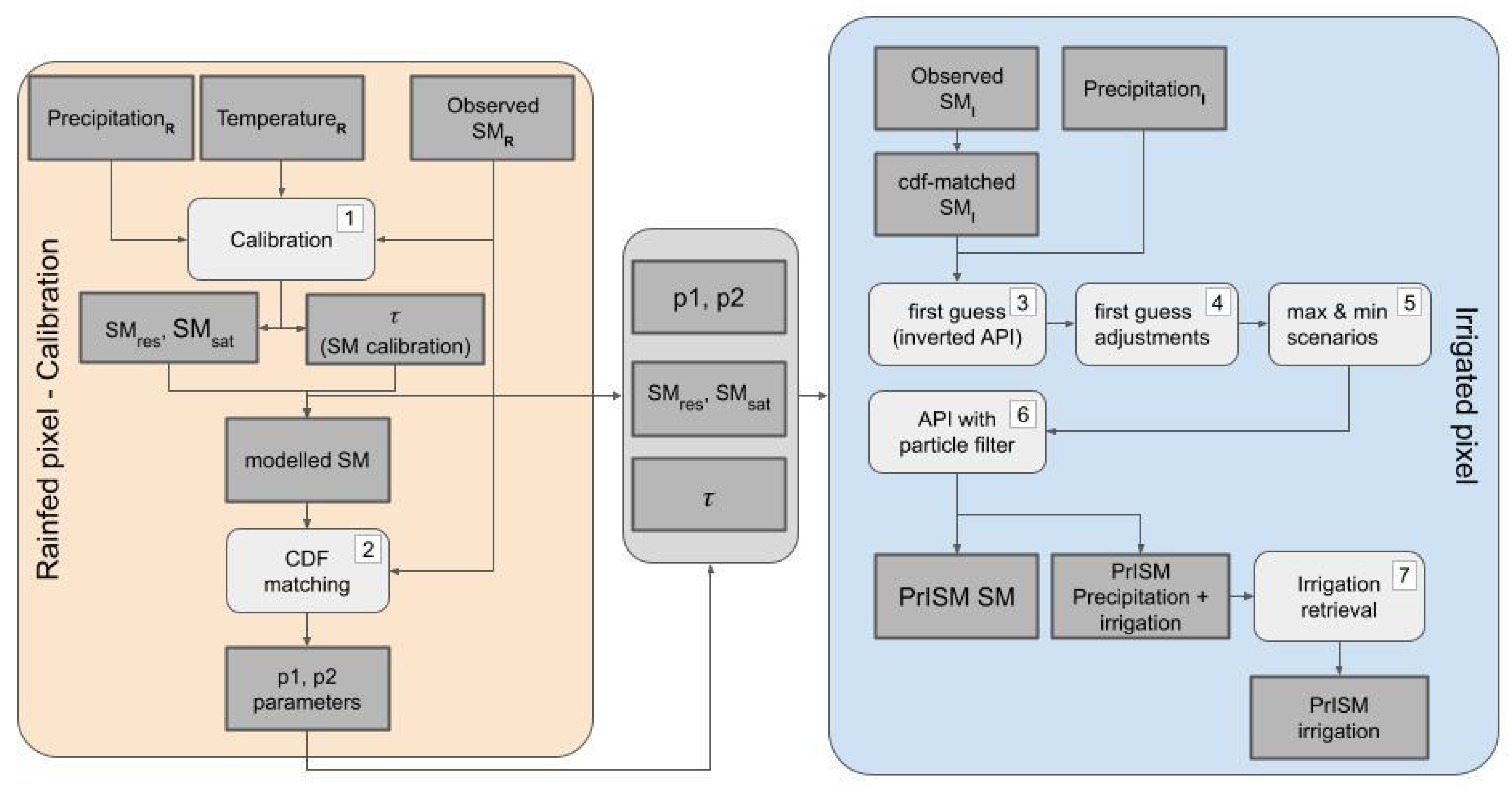
The new PrISM methodology for irrigation estimation can be summarized by the following steps:

1.

Calibration: The few parameters ($\tau ,S{M}_{res},S{M}_{sat}$) of the API equation are calibrated using remote-sensing soil moisture observations of rainfed areas.

2.

CDF-matching: A CDF (cumulative distribution function) matching between soil moisture observed in the rainfed area and the soil moisture profile retrieved from PrISM is performed in order to harmonize the model with the data. Two parameters $p_1$ and $p_2$ are retrieved and applied to SM observations in the irrigated pixels.

3.

First Guess: The inverse API formula is used directly on observed SM data from the irrigated pixel to create irrigation events.

4.

First Guess adjustments: The first guess is adjusted to account for the irrigation system (by constraining the maximum amounts of irrigation events that can happen during a defined amount of time).

5.

Maximum and minimum scenario: From the first guess maximum and minimum initial guesses are built, which will produce the two different scenarios. These guesses are based on the two extreme positions where the irrigation event is placed: right after a SM observation (maximum scenario) or right before the following one (minimum scenario).

6.

Particle filter: The first guess containing precipitation and irrigation profile is perturbed using the particle filter assimilation technique. For each perturbed guess, the API formula is used to create a corresponding perturbed SM profile, which is then compared with the observed SM to select the closest match. This comparison is performed every 5 consecutive SM observations, whenever they are available, in a rolling window fashion. For each window, only the closest n-particles are kept and a final average is performed among all the windows to retrieve the final irrigation and precipitation profile.

7.

Irrigation retrieval: Irrigation and precipitation profiles derived from the particle filter assimilation scheme are separated, using the original input precipitation profile to distinguish them.

Figure 3 shows the main steps listed above together with the input variables required to run PrISM.

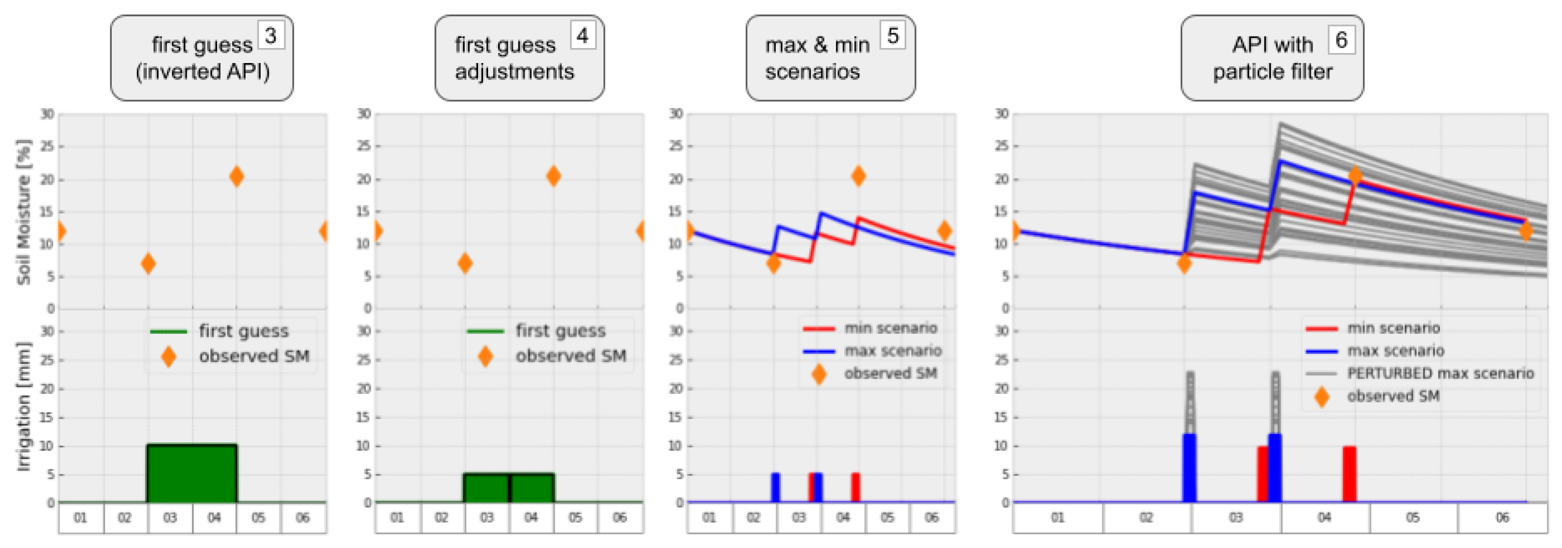
One of the main elements of this methodology is the creation and processing of the first guess. The first guess is an initial estimation of the irrigation profile (which is computed before the particle filter assimilates the $SM$ observations) and it can be constrained so that irrigation events have a precise frequency, which is derived from the different irrigation systems installed. Adding information in PrISM about the expected frequencies of irrigation helps to increase the precision of the final estimation of irrigation, avoiding large underestimations of total irrigation amounts, as shown in Paolini et al. [45]. The frequency of irrigation is assumed to vary for the different irrigation systems: while it is set to daily for modern systems such as sprinkler and drip, the irrigation frequency is assumed to be weekly for flood irrigation.

PrISM does not only retrieve a set of single punctual estimations of irrigation amounts, but it also provides a confidence interval, which is the result of the maximum and minimum scenario simulations that are run sequentially by the algorithm. These two simulations provide a range of estimations that define the maximum and minimum amount of irrigation detected by the $SM$ observations. Figure 4 represents a visualization of all the steps required to create a first guess and retrieve the final estimations for the minimum and maximum scenario, assuming that the simulation is run for sprinkler irrigation, with a daily frequency. More details about the modified PrISM methodology for irrigation estimation can be found in Paolini et al. [45], while the PrISM methodology is introduced and detailed in Pellarin et al. [57] and Pellarin et al. [58].

3. Results

PrISM was applied to each of the three irrigation districts with different predominant irrigation systems and it was validated using the water meters installed in Algerri-Balaguer and Canals d’Urgell. Calibration was performed for each district in nearby rainfed areas.

3.1. Flood Irrigation: Canals d’Urgell

The Canals d’Urgell district is predominantly irrigated through flood irrigation, thus results are produced constraining the first guess to contain a maximum of one irrigation event per week. Irrigation amounts are produced from PrISM for each 1 km pixel with a 3 h temporal frequency. These resulting amounts are then averaged for each of the two distinct areas of Canals d’Urgell and aggregated at a weekly scale to be compared with the in situ amounts collected by the water meters at the beginning of each of the two canals. Figure 5 and Figure 6 show the results for the main and auxiliary canals, respectively. Results from PrISM are shown as confidence intervals between the maximum and minimum scenarios simulated by the PrISM algorithm. When comparing PrISM results against in situ data, the irrigation amounts predicted by this methodology show a bias of $-4.81$ mm/week, a root mean square error (rmse) of $10.05$ mm/week and a Pearson’s correlation coefficient of $0.58$ (p-value = $3.1\times {10}^{-33}$). The auxiliary canal generally shows lower amounts of irrigation compared to the main canal and a similar seasonal trend throughout the years, with the largest amount of water transported steadily during the summer. PrISM shows the following metrics when compared to the in situ data for the area fed by the auxiliary canal: bias of $0.43$ mm/week, rmse of $6.88$ mm/week and Pearson’s correlation coefficient of $0.73$ (p-value = $2.07\times {10}^{-60}$).

3.2. Sprinkler Irrigation: Algerri Balaguer

To simulate irrigation practices under a sprinkler irrigation scenario, PrISM was constrained to produce irrigation guesses with a daily frequency. The calibration was first run in a rainfed area located nearby and results were then compared with the water meter installed at the beginning of the canal. Results show good agreement with in situ data, with a bias of $1.07$ mm, a rmse of $8.06$, and a Pearson’s correlation coefficient of $0.76$ (p-value = $6.7\times {10}^{-60}$) for the entire time series. Figure 7 shows a comparison of time series of weekly and cumulative irrigation amounts between in situ data and PrISM results, together with the linear correlation between these two quantities.

3.3. Drip Irrigation: Segria Sud

Drip is a modern irrigation system that is assumed to be active with a daily to sub-daily frequency. For this reason, as for the sprinkler irrigation system, PrISM was constrained with daily irrigation frequency. Similarly to the previously analyzed irrigation district, before running PrISM over the district, calibration was performed on a nearby rainfed area. This district is not uniformly irrigated, and many fields are rainfed, especially on the east side, according to the administrative database of Catalunya (https://agricultura.gencat.cat/ca/ambits/desenvolupament-rural/sigpac/mapa-cultius/, last accessed 15 January 2024) and the map of irrigation systems directly retrieved from remote-sensing data [59]. Figure 8A shows the percentage of irrigated areas for each pixel of the 1 km grid from the $SM$ input. For the analysis of the results, only irrigation amounts from pixels with over 50% of irrigated areas were considered (corresponding to the pixels with the green edge color in Figure 8A). In situ irrigation amounts at a weekly scale were not available for this district, but the total water allocation established by the irrigation managers is set to be around 200 mm/year. Figure 9 shows irrigation amounts retrieved by PrISM for the district of Segria Sud.

4. Discussion

4.1. Flood Irrigation: Canals d’Urgell

When analyzing the results for the Urgell irrigation district, it is worth noticing how PrISM can correctly depict the drastic change in total irrigation amount that occurred in 2023 for the area fed by the main canal, subjected to strong restrictions in terms of the water supply. According to in situ data, annual irrigation volumes were reduced from an average of around 540 ${\mathrm{hm}}^3$ (equivalent to 855 mm) during the previous regular years to 180 ${\mathrm{hm}}^3$ (or 287 mm) for 2023, which corresponds to only the $33\%$ of the normal irrigation volume. Similarly, PrISM shows a decrease from 550 mm in regular years to 297 mm for 2023, corresponding to the $57\%$ of the normal irrigation volume. The amount detected in 2023 is comparable to in situ estimates, but for previous years PrISM estimates show instead lower irrigation volumes than the in situ ground truth. Underestimation of irrigation amounts can be mainly caused by two factors: saturation of the soil during the irrigation event due to overirrigation and rapid drying of the surface soil layer between two irrigation events. Firstly, flood irrigation, which is predominant in this area, is characterized by a large amount of water distributed in the field during each irrigation event and overirrigation might be a common practice in the area. This leads to saturation of the soil, which causes a higher amount of water drainage as well as evaporation, and it is not completely accounted for by PrISM since it is not visible from the observed surface $SM$. Secondly, observed $SM$ from satellite observations only represents the first shallow layer of the soil, which dries much faster than the root zone $SM$, especially for flood irrigation practices that occur sporadically. For this reason, the full amount of irrigation is quite difficult to retrieve using surface $SM$ only. Regarding the auxiliary canal, PrISM shows instead quite accurate results, with a steady value for total irrigated amounts of around 500 mm throughout all the years. This canal was not subject to any restriction in 2023 and it is possible to notice how similar amounts to previous years are reported. Fields in this area receive a lower irrigation amount and they are not over-irrigated, resulting in a more accurate retrieval of irrigation amounts. In summary, PrISM is unable to precisely estimate large irrigation amounts over areas subject to overirrigation, and it is better suited to estimate irrigation at lower amounts, as is the case for the area fed by the auxiliary canal, and for the area fed by the main canal for the year 2023, when overirrigation was not possible due to water shortages, and PrISM performances were optimal.

PrISM shows excellent performances when compared with similar methodologies applied in the areas of previous studies. Dari et al. [27] retrieved irrigation estimation every 5 days using the SM2RAIN algorithm, and estimated a rmse of $4.37$ mm/5-days and correlation r = $0.73$ for the Urgell area. The analysis is performed using the same input data, Dispatch SM at 1 km but only for the years 2016 and 2017, which shows large gaps in terms of in situ data. These values are quite comparable to the performances shown in this work, even though this work proposed a longer time series and it also comprises 2023, a year with large anomalies in terms of total irrigation amounts. When converted to a 5-day temporal range and aggregated for the entire Urgell area, PriSM shows a $rmse$ of $7.07$ mm/5-day and a Pearson’s correlation of $0.6$. This confirms the robustness of the PrISM approach, which keeps similar performances over a long range of time. Dari et al. [29] applied SM2RAIN again over the Urgell irrigation district but for a longer time range, from 2017 to 2020 retrieving worse performances over the area, with a rmse of $14.66$ mm/14-days and a correlation r = $0.53$. PrISM shows a comparable rmse of $16.39$ mm/14-days and a higher correlation r = $0.70$ when results from PrISM are converted to the same temporal extension and spatial aggregation (joining the two principal and auxiliary areas together). PrISM also shows better performances when compared to an ET-based methodology, such as the one proposed by Brombacher et al. [37] and applied over the Urgell district. For this particular area, the authors show no statistically significant results when comparing monthly and seasonal water use with in situ data at field level, for three different test plots. The main difficulty is identified by the authors to be the absence of enough hydrological similar pixels in the area.

4.2. Sprinkler Irrigation: Algerri Balaguer

As shown in previous studies on irrigation estimation focused in this area [29,31,32,45], results are quite satisfactory in this area and performances are quite similar even when using different methodologies and different remote-sensing datasets. The district is irrigated quite uniformly and most fields are equipped with sprinklers, which irrigate almost daily with a proper amount, close to the optimal plant water need. Irrigation amounts from sprinklers are easier to detect from SM estimates since the topsoil layer is kept almost uniformly and constantly wet by this irrigation system.

Laluet et al. [32] compared SM2RAIN with the methodology proposed by their study over the Algerri-Balaguer area, which implements a SM-based calibration in the FAO-56 model. The comparison shows how the FAO-56 approach is outperforming SM2RAIN in 2019 over Algerri-Balaguer, showing an RMSE, bias, and correlation r values of $6.6$ mm/week, $-0.06$ mm/week and $0.88$, against $9.7$ mm/week, $-3.3$ mm/week and $0.65$ of SM2RAIN. As indicated in Figure 7, the performances of PrISM are in-between the two methodologies, showing better results than PrISM but a slightly worse performance than the FAO-56 approach, which is run at field-level and considers only irrigated fields, thus it is based on a more intensive data preparation and a different spatial scale. Overall results are expected to be similar when PrISM is run at a field scale like the FAO-56 approach, and the validation is still performed on aggregated data at the district scale. The district of Algerri-Balaguer is also used as a study area in Kragh et al. [25] to estimate irrigation from different approaches (using SM and Evapotranspiration as inputs). Even though a quantitative analysis against in situ benchmark data is not presented in the study, large underestimations of irrigation amounts are reported for all of the proposed approaches.

4.3. Drip Irrigation: Segria Sud

For the case of the Segria irrigation district, mainly irrigated by drip systems, it is noticeable how total annual irrigation amounts predicted by PrISM are consistently lower than the declared amount of allocated water for the district, with around 40 to 60% of irrigation amounts that go undetected by this remote-sensing product. This suggests a strong underestimation of the irrigation amounts, which is also visible from the weekly time series of irrigation amounts. This time series shows almost no irrigation during the summer period and some peaks during winter, which are precipitation wrongly mislabeled as irrigation. The main reasons that caused this large underestimation of irrigation amounts are attributed to the very weak irrigation signal contained in the $SM$ data. Since the area is not homogeneously irrigated, $SM$ contains an averaged signal from dryland and irrigated fields which weakens the irrigation signal, as it was proven in previous synthetic experiments [40,44,45]. Furthermore, drip irrigation is applied very locally near the plant and in small amounts. In addition, since water allocation is usually below potential crop water requirements, most of the crops in this area are under deficit irrigation for long periods and water is only applied in moments of very high water stress. This is also a clear cause of the failure in irrigation detection in this area. Drip irrigation is not easily detectable by $SM$, given its very localized nature and the very low amount of water fed to the plants. Figure 8B shows an example from one pixel in the Segria-Sud district that contains the highest percentage of irrigated areas (around 70%). It is clear how during the driest period, observed $SM$ does not show any variation due to irrigation and the values constantly stay close to a residual value of $SM$. The few more meaningful irrigation events are placed in winter and are probably precipitation events not present in the original dataset and thus not removed correctly from the final product. This demonstrates that drip irrigation practices are the most difficult to estimate in terms of irrigation amounts using remote-sensing $SM$ data. In the future, the use of higher resolution $SM$ satellite products together with complementary products such as actual plant evapotranspiration $ET$ and root zone $SM$ will greatly improve the estimation of irrigation amounts for this irrigation system.

5. Conclusions

This study investigates the performances of PrISM in estimating irrigation amounts for 3 different irrigation districts in Catalunya, irrigated through different irrigation systems: flood, sprinkler, and drip. Irrigation estimates were produced for 7 years, including 2023, where a large long-term drought intensified in the region and forced authorities to restrict water usage during summer months. For the district of Canals d’Urgell, mostly irrigated through flood irrigation, validation with in situ data was performed aggregating the PrISm results over two areas: the area fed by the main canal and the area fed by the auxiliary canal. The main canal provides the fields with the largest quantities of water (for all the years except for 2023 when restrictions were imposed) and comparison with in situ data resulted in a moderate correlation, mainly caused by a large underestimation of irrigation amounts for the years where no restrictions where imposed. During 2023 the amount of water available to each field strongly decreased and PrISM showed better performances, suggesting that underestimation during previous years was linked with overirrigation and large drainage that cannot be detected in the $SM$ signal. The area fed by the auxiliary canal showed instead daily good and stable performances when validated against in situ data, motivated by the fact that fields are subjected to a lower amount of irrigation. Algerri-Balaguer, the district irrigated mostly with sprinklers, showed the best results when compared to in situ data. These results are justified by the fact that sprinkler irrigation is spread homogeneously in the field and with a moderate constant amount, which leaves the soil generally wet and it is easily detected by the $SM$ product. Conversely, irrigation amounts were hardly detected in the district irrigated by drip systems, given that these systems use low amounts of irrigation and in a very localized manner, mostly at the plant’s base, which goes undetected in the $SM$ signal. Additionally, the district is not entirely irrigated, with large areas inside the pixels that are rainfed, which in turn decreases the sensitivity of the $SM$ to irrigation.

This study shows the capability and limitations of retrieving irrigation from remotely sensed $SM$ under different irrigation systems and different climatic scenarios. PrISM captured changes in water amounts after restrictions were enacted for 2023 in different areas in the region and distinguished which areas were facing restrictions. In particular, a decrease in irrigation amounts of $49\%$ was detected in the area most affected by the restriction, Canals D’Urgell. This estimate is lower, but close to the official value derived from in situ data, which estimated the change to be around $66.7\%$ thus providing an additional validation of the capabilities of PrISM. Multi-annual validation against in situ data of total water use showed how PrISM is a robust methodology, capable of adapting to sudden changes in irrigation practices, which are typical and consequences of drought periods. Furthermore, this study quantitatively assessed the relationship between the capability of remote sensing data to detect irrigation amounts and the irrigation systems installed. Studying different irrigation districts with different irrigation systems predominantly installed allowed to highlight how irrigation amounts are easily detectable from sprinkler and flood irrigation systems, while it is still challenging to correctly detect and estimate irrigation under drip irrigation systems. Future works might focus on improving the capabilities of detecting irrigation for the drip localized system: using remote-sensing data at higher spatial scales might help to distinguish irrigated from rainfed fields while integrating different hydrological variables such as $ET$ and root-zone $SM$ might help to increase the sensitivity of the approach to lower irrigation amounts.

References

- Reilly, J.; Tubiello, F.; McCarl, B.; Abler, D.; Darwin, R.; Fuglie, K.; Hollinger, S.; Izaurralde, C.; Jagtap, S.; Jones, J. US agriculture and climate change: New results. Clim. Chang. 2003, 57, 43–67. [Google Scholar] [CrossRef]
- Parry, M.L.; Rosenzweig, C.; Iglesias, A.; Livermore, M.; Fischer, G. Effects of climate change on global food production under SRES emissions and socio-economic scenarios. Glob. Environ. Chang. 2004, 14, 53–67. [Google Scholar] [CrossRef]
- Howden, S.M.; Soussana, J.F.; Tubiello, F.N.; Chhetri, N.; Dunlop, M.; Meinke, H. Adapting agriculture to climate change. Proc. Natl. Acad. Sci. USA 2007, 104, 19691–19696. [Google Scholar] [CrossRef] [PubMed]
- Schlenker, W.; Lobell, D.B. Robust negative impacts of climate change on African agriculture. Environ. Res. Lett. 2010, 5, 014010. [Google Scholar] [CrossRef]
- Madadgar, S.; AghaKouchak, A.; Farahmand, A.; Davis, S.J. Probabilistic estimates of drought impacts on agricultural production. Geophys. Res. Lett. 2017, 44, 7799–7807. [Google Scholar] [CrossRef]
- IPCC. Climate Change 2021: The Physical Science Basis. Contribution of Working Group I to the Sixth Assessment Report of the Intergovernmental Panel on Climate Change; Masson-Delmotte, V., Zhai, P., Pirani, A., Connors, S.L., Péan, C., Berger, S., Caud, N., Chen, Y., Goldfarb, L., Gomis, M.I., et al., Eds.; Cambridge University Press: Cambridge, UK; New York, NY, USA, 2021; Volume 1. [Google Scholar] [CrossRef]
- Douville, H.; Raghavan, K.; Renwick, J.; Allan, R.P.; Arias, P.A.; Barlow, M.; Cerezo-Mota, R.; Cherchi, A.; Gan, T.Y.; Gergis, J. Water cycle changes. In Climate Change 2021: The Physical Science Basis. Contribution of Working Group I to the Sixth Assessment Report of the Intergovernmental Panel on Climate Change; Masson-Delmotte, V., Zhai, P., Pirani, A., Connors, S.L., Péan, C., Berger, S., Caud, N., Chen, Y., Goldfarb, L., Gomis, M.I., et al., Eds.; Cambridge University Press: Cambridge, UK; New York, NY, USA, 2021; pp. 1055–1210. [Google Scholar]
- Toreti, A.; Bavera, D.; Acosta, N.J.; Arias-Muñoz, C.; Barbosa, P.; De, J.A.; Di, C.C.; Fioravanti, G.; Grimaldi, S.; Hrast, E.A.; et al. Drought in the western Mediterranean—May 2023; Publications Office of the European Union: Luxembourg, 2023; EUR 31555 EN; ISBN 9789268045183. [Google Scholar] [CrossRef]
- Vanneuville, W.; Werner, B.; Kjeldsen, T.; Miller, J.; Kossida, M.; Tekidou, A.; Kakava, A.; Crouzet, P. Water Resources in Europe in the Context of Vulnerability: EEA 2012 State of Water Assessment; European Environment Agency: Copenhagen, Denmark, 2012. [Google Scholar]
- Baruth, B.; Bassu, S.; Ben, A.W.; Biavetti, I.; Bratu, M.; Cerrani, I.; Chemin, Y.; Claverie, M.; De, P.P.; Fumagalli, D.; et al. JRC MARS Bulletin—Crop Monitoring in Europe—May 2023; Publications Office of the European Union: Luxembourg, 2023; Volume 31, ISSN 2443-8278. [Google Scholar] [CrossRef]
- Lemus-Canovas, M.; Insua-Costa, D.; Trigo, R.M.; Miralles, D.G. Record-shattering 2023 Spring heatwave in western Mediterranean amplified by long-term drought. NPJ Clim. Atmos. Sci. 2024, 7, 25. [Google Scholar] [CrossRef]
- NFORME DE LA SEQUÍA DE 2023 presentado en la Junta de Gobierno de 21/12/2023 para recibir aportaciones [Report on the drought of 2023]. Memoria 7. In Proceedings of the Confederación Hidrográfica del Ebro (CHE), Zaragoza, Spain, 21 December 2023.
- FAO. AQUASTAT—FAO’s Global Information System on Water and Agriculture; FAO: Nairobi, Kenya, 2023. [Google Scholar]
- Foley, J.A.; Ramankutty, N.; Brauman, K.A.; Cassidy, E.S.; Gerber, J.S.; Johnston, M.; Mueller, N.D.; O’Connell, C.; Ray, D.K.; West, P.C. Solutions for a cultivated planet. Nature 2011, 478, 337–342. [Google Scholar] [CrossRef] [PubMed]
- Gleick, P.H.; Allen, L.; Christian-Smith, J.; Cohen, M.J.; Cooley, H.; Heberger, M.; Morrison, J.; Palaniappan, M.; Schulte, P. The World’s Water Volume 7: The Biennial Report on Freshwater Resources; Island Press: Washington, DC, USA, 2012. [Google Scholar]
- United Nations Environment Programme/Mediterranean Action Plan; Plan Bleau. State of the Environment and Development in the Mediterranean; Food & Agriculture Org.: Nairobi, Kenya, 2020. [Google Scholar]
- Massari, C.; Modanesi, S.; Dari, J.; Gruber, A.; De Lannoy, G.J.M.; Girotto, M.; Quintana-Seguí, P.; Le Page, M.; Jarlan, L.; Zribi, M.; et al. A Review of Irrigation Information Retrievals from Space and Their Utility for Users. Remote Sens. 2021, 13, 4112. [Google Scholar] [CrossRef]
- Thenkabail, P.S.; Biradar, C.M.; Noojipady, P.; Dheeravath, V.; Li, Y.; Velpuri, M.; Gumma, M.; Gangalakunta, O.R.P.; Turral, H.; Cai, X. Global irrigated area map (GIAM), derived from remote sensing, for the end of the last millennium. Int. J. Remote Sens. 2009, 30, 3679–3733. [Google Scholar] [CrossRef]
- Portmann, F.T.; Siebert, S.; Döll, P. MIRCA2000—Global monthly irrigated and rainfed crop areas around the year 2000: A new high-resolution data set for agricultural and hydrological modeling. Glob. Biogeochem. Cycles 2010, 24. [Google Scholar] [CrossRef]
- Salmon, J.M.; Friedl, M.A.; Frolking, S.; Wisser, D.; Douglas, E.M. Global rain-fed, irrigated, and paddy croplands: A new high resolution map derived from remote sensing, crop inventories and climate data. Int. J. Appl. Earth Obs. Geoinf. 2015, 38, 321–334. [Google Scholar] [CrossRef]
- Beltran, C.M.; Belmonte, A.C. Irrigated crop area estimation using Landsat TM imagery in La Mancha, Spain. Photogramm. Eng. Remote Sens. 2001, 67, 1177–1184. [Google Scholar]
- Thenkabail, P.S.; Schull, M.; Turral, H. Ganges and Indus river basin land use/land cover (LULC) and irrigated area mapping using continuous streams of MODIS data. Remote Sens. Environ. 2005, 95, 317–341. [Google Scholar] [CrossRef]
- Ozdogan, M.; Gutman, G. A new methodology to map irrigated areas using multi-temporal MODIS and ancillary data: An application example in the continental US. Remote Sens. Environ. 2008, 112, 3520–3537. [Google Scholar] [CrossRef]
- Zribi, M.; Baghdadi, N.; Bousbih, S.; El-Hajj, M.; Gao, Q. Surface Moisture And Irrigation Mapping At Agricultural Field Scale Using The Synergy Sentinel-1/Sentinel-2 Data. Int. Arch. Photogramm. Remote Sens. Spat. Inf. Sci. 2019, XLII-3-W6, 357–361. [Google Scholar] [CrossRef]
- Kragh, S.J.; Dari, J.; Modanesi, S.; Massari, C.; Brocca, L.; Fensholt, R.; Stisen, S.; Koch, J. An Inter-Comparison of Approaches and Frameworks to Quantify Irrigation from Satellite Data. Hydrol. Earth Syst. Sci. 2024, 28, 441–457. [Google Scholar] [CrossRef]
- Brocca, L.; Tarpanelli, A.; Filippucci, P.; Dorigo, W.; Zaussinger, F.; Gruber, A.; Fernández-Prieto, D. How much water is used for irrigation? A new approach exploiting coarse resolution satellite soil moisture products. Int. J. Appl. Earth Obs. Geoinf. 2018, 73, 752–766. [Google Scholar] [CrossRef]
- Dari, J.; Brocca, L.; Quintana-Seguí, P.; Escorihuela, M.J.; Stefan, V.; Morbidelli, R. Exploiting High-Resolution Remote Sensing Soil Moisture to Estimate Irrigation Water Amounts over a Mediterranean Region. Remote Sens. 2020, 12, 2593. [Google Scholar] [CrossRef]
- Dari, J.; Quintana-Seguí, P.; Morbidelli, R.; Saltalippi, C.; Flammini, A.; Giugliarelli, E.; Escorihuela, M.J.; Stefan, V.; Brocca, L. Irrigation estimates from space: Implementation of different approaches to model the evapotranspiration contribution within a soil-moisture-based inversion algorithm. Agric. Water Manag. 2022, 265, 107537. [Google Scholar] [CrossRef]
- Dari, J.; Brocca, L.; Modanesi, S.; Massari, C.; Tarpanelli, A.; Barbetta, S.; Quast, R.; Vreugdenhil, M.; Freeman, V.; Barella-Ortiz, A.; et al. Regional data sets of high-resolution (1 and 6 km) irrigation estimates from space. Earth Syst. Sci. Data 2023, 15, 1555–1575. [Google Scholar] [CrossRef]
- Garrido-Rubio, J.; González-Piqueras, J.; Campos, I.; Osann, A.; González-Gómez, L.; Calera, A. Remote Sensing–Based Soil Water Balance for Irrigation Water Accounting at Plot and Water User Association Management Scale. Agric. Water Manag. 2020, 238, 106236. [Google Scholar] [CrossRef]
- Olivera-Guerra, L.E.; Laluet, P.; Altés, V.; Ollivier, C.; Pageot, Y.; Paolini, G.; Chavanon, E.; Rivalland, V.; Boulet, G.; Villar, J.M.; et al. Modeling actual water use under different irrigation regimes at district scale: Application to the FAO-56 dual crop coefficient method. Agric. Water Manag. 2023, 278, 108119. [Google Scholar] [CrossRef]
- Laluet, P.; Olivera-Guerra, L.E.; Altés, V.; Paolini, G.; Ouaadi, N.; Rivalland, V.; Jarlan, L.; Villar, J.M.; Merlin, O. Retrieving the Irrigation Actually Applied at District Scale: Assimilating High-Resolution Sentinel-1-derived Soil Moisture Data into a FAO-56-based Model. Agric. Water Manag. 2024, 293, 108704. [Google Scholar] [CrossRef]
- Wei, S.; Xu, T.; Niu, G.Y.; Zeng, R. Estimating Irrigation Water Consumption Using Machine Learning and Remote Sensing Data in Kansas High Plains. Remote Sens. 2022, 14, 3004. [Google Scholar] [CrossRef]
- Zaussinger, F.; Dorigo, W.; Gruber, A.; Tarpanelli, A.; Filippucci, P.; Brocca, L. Estimating irrigation water use over the contiguous United States by combining satellite and reanalysis soil moisture data. Hydrol. Earth Syst. Sci. 2019, 23, 897–923. [Google Scholar] [CrossRef]
- Zohaib, M.; Kim, H.; Choi, M. Detecting global irrigated areas by using satellite and reanalysis products. Sci. Total. Environ. 2019, 677, 679–691. [Google Scholar] [CrossRef] [PubMed]
- Droogers, P.; Immerzeel, W.W.; Lorite, I.J. Estimating actual irrigation application by remotely sensed evapotranspiration observations. Agric. Water Manag. 2010, 97, 1351–1359. [Google Scholar] [CrossRef]
- Brombacher, J.; Silva, I.R.d.O.; Degen, J.; Pelgrum, H. A novel evapotranspiration based irrigation quantification method using the hydrological similar pixels algorithm. Agric. Water Manag. 2022, 267, 107602. [Google Scholar] [CrossRef]
- Zhang, C.; Long, D. Estimating Spatially Explicit Irrigation Water Use Based on Remotely Sensed Evapotranspiration and Modeled Root Zone Soil Moisture. Water Resour. Res. 2021, 57, e2021WR031382. [Google Scholar] [CrossRef]
- Modanesi, S.; Massari, C.; Bechtold, M.; Lievens, H.; Tarpanelli, A.; Brocca, L.; Zappa, L.; De Lannoy, G.J.M. Challenges and benefits of quantifying irrigation through the assimilation of Sentinel-1 backscatter observations into Noah-MP. Hydrol. Earth Syst. Sci. 2022, 26, 4685–4706. [Google Scholar] [CrossRef]
- Abolafia-Rosenzweig, R.; Livneh, B.; Small, E.; Kumar, S. Soil Moisture Data Assimilation to Estimate Irrigation Water Use. J. Adv. Model. Earth Syst. 2019, 11, 3670–3690. [Google Scholar] [CrossRef]
- Jalilvand, E.; Abolafia-Rosenzweig, R.; Tajrishy, M.; Kumar, S.V.; Mohammadi, M.R.; Das, N.N. Is It Possible to Quantify Irrigation Water-Use by Assimilating a High-Resolution Satellite Soil Moisture Product? Water Resour. Res. 2023, 59, e2022WR033342. [Google Scholar] [CrossRef]
- Pan, F.; Peters-Lidard, C.D.; Sale, M.J. An analytical method for predicting surface soil moisture from rainfall observations. Water Resour. Res. 2003, 39. [Google Scholar] [CrossRef]
- Escorihuela, M.J.; Quintana-Seguí, P. Comparison of remote sensing and simulated soil moisture datasets in Mediterranean landscapes. Remote Sens. Environ. 2016, 180, 99–114. [Google Scholar] [CrossRef]
- Zappa, L.; Schlaffer, S.; Brocca, L.; Vreugdenhil, M.; Nendel, C.; Dorigo, W. How accurately can we retrieve irrigation timing and water amounts from (satellite) soil moisture? Int. J. Appl. Earth Obs. Geoinf. 2022, 113, 102979. [Google Scholar] [CrossRef]
- Paolini, G.; Escorihuela, M.J.; Merlin, O.; Laluet, P.; Bellvert, J.; Pellarin, T. Estimating multi-scale irrigation amounts using multi-resolution soil moisture data: A data-driven approach using PrISM. Agric. Water Manag. 2023, 290, 108594. [Google Scholar] [CrossRef]
- Merlin, O.; Escorihuela, M.J.; Mayoral, M.A.; Hagolle, O.; Al Bitar, A.; Kerr, Y. Self-calibrated evaporation-based disaggregation of SMOS soil moisture: An evaluation study at 3km and 100m resolution in Catalunya, Spain. Remote Sens. Environ. 2013, 130, 25–38. [Google Scholar] [CrossRef]
- Oiha, N.; Merlin, O.; Molero, B.; Sucre, C.; Olivera, L.; Rivalland, V.; Er-Raki, S. Sequential Downscaling of the SMOS Soil Moisture at 100 M Resolution Via a Variable Intermediate Spatial Resolution. In Proceedings of the IGARSS 2018—2018 IEEE International Geoscience and Remote Sensing Symposium, Valencia, Spain, 22–27 July 2018; pp. 3735–7003. [Google Scholar] [CrossRef]
- Merlin, O.; Rudiger, C.; Al Bitar, A.; Richaume, P.; Walker, J.P.; Kerr, Y.H. Disaggregation of SMOS Soil Moisture in Southeastern Australia. IEEE Trans. Geosci. Remote Sens. 2012, 50, 1556–1571. [Google Scholar] [CrossRef]
- Ojha, N.; Merlin, O.; Suere, C.; Escorihuela, M.J. Extending the Spatio-Temporal Applicability of DISPATCH Soil Moisture Downscaling Algorithm: A Study Case Using SMAP, MODIS and Sentinel-3 Data. Front. Environ. Sci. 2021, 9. [Google Scholar] [CrossRef]
- Molero, B.; Merlin, O.; Malbéteau, Y.; Al Bitar, A.; Cabot, F.; Stefan, V.; Kerr, Y.; Bacon, S.; Cosh, M.; Bindlish, R.; et al. SMOS disaggregated soil moisture product at 1 km resolution: Processor overview and first validation results. Remote Sens. Environ. 2016, 180, 361–376. [Google Scholar] [CrossRef]
- Merlin, O.; Malbéteau, Y.; Notfi, Y.; Bacon, S.; Khabba, S.E.R.S.; Jarlan, L. Performance Metrics for Soil Moisture Downscaling Methods: Application to DISPATCH Data in Central Morocco. Remote Sens. 2015, 7, 3783–3807. [Google Scholar] [CrossRef]
- Duan, Z.; Liu, J.; Tuo, Y.; Chiogna, G.; Disse, M. Evaluation of eight high spatial resolution gridded precipitation products in Adige Basin (Italy) at multiple temporal and spatial scales. Sci. Total. Environ. 2016, 573, 1536–1553. [Google Scholar] [CrossRef] [PubMed]
- Tang, G.; Clark, M.P.; Papalexiou, S.M.; Ma, Z.; Hong, Y. Have satellite precipitation products improved over last two decades? A comprehensive comparison of GPM IMERG with nine satellite and reanalysis datasets. Remote Sens. Environ. 2020, 240, 111697. [Google Scholar] [CrossRef]
- Maneewongvatana, S.; Mount, D.M. Analysis of approximate nearest neighbor searching with clustered point sets. arXiv 1999, arXiv:cs/9901013. [Google Scholar]
- Pellarin, T.; Ali, A.; Chopin, F.; Jobard, I.; Bergès, J.C. Using spaceborne surface soil moisture to constrain satellite precipitation estimates over West Africa. Geophys. Res. Lett. 2008, 35. [Google Scholar] [CrossRef]
- Román-Cascón, C.; Pellarin, T.; Gibon, F.; Brocca, L.; Cosme, E.; Crow, W.; Fernández-Prieto, D.; Kerr, Y.H.; Massari, C. Correcting satellite-based precipitation products through SMOS soil moisture data assimilation in two land-surface models of different complexity: API and SURFEX. Remote Sens. Environ. 2017, 200, 295–310. [Google Scholar] [CrossRef]
- Pellarin, T.; Louvet, S.; Gruhier, C.; Quantin, G.; Legout, C. A simple and effective method for correcting soil moisture and precipitation estimates using AMSR-E measurements. Remote Sens. Environ. 2013, 136, 28–36. [Google Scholar] [CrossRef]
- Pellarin, T.; Román-Cascón, C.; Baron, C.; Bindlish, R.; Brocca, L.; Camberlin, P.; Fernández-Prieto, D.; Kerr, Y.H.; Massari, C.; Panthou, G.; et al. The Precipitation Inferred from Soil Moisture (PrISM) Near Real-Time Rainfall Product: Evaluation and Comparison. Remote Sens. 2020, 12, 481. [Google Scholar] [CrossRef]
- Paolini, G.; Escorihuela, M.J.; Merlin, O.; Sans, M.P.; Bellvert, J. Classification of Different Irrigation Systems at Field Scale Using Time-Series of Remote Sensing Data. IEEE J. Sel. Top. Appl. Earth Obs. Remote Sens. 2022, 15, 10055–10072. [Google Scholar] [CrossRef]
Figure 1.
Map of the study area and the three irrigation districts considered in this study: Canals d’Urgell, Algerri-Balaguer, and Segria Sud. For each irrigation district, the distribution of the different irrigation types is shown in a pie chart. Data from SIGPAC.
Figure 2.
Representation of the in situ data used for this study. (A) Spatial distribution of the water meters installed in Algerri-Balaguer and Canals d’Urgell (yellow crosses), together with the footprint of the canal systems and the meteo stations (red dots). (B–D) Weekly evolution of the irrigation amounts registered by the water meters in the districts for the years from 2016 to 2023 (2023 is depicted in green to underline the differences in water supply, while the other years from 2016 to 2022 are in grey).
Figure 3.
Flowchart of the PrISM methodology representing the main steps. Numbers in each box correspond to the main operation required to estimate irrigation, as listed and explained in the text.
Figure 4.
Visualization of the main step of PrISM (corresponding to numbers 3 to 6 of the methodology flowchart) needed to create a first guess of irrigation and a final estimation of the two scenarios. The visualization assumes daily irrigation, typical of modern irrigation systems such as sprinklers and drips.
Figure 5.
Comparison of irrigation amounts produced by PrISM against in situ data from 2016 to 2023 for the area of the Canals d’Urgell district fed by the main canal. (A) shows time series of in situ and retrieved irrigation amounts expressed in mm/week, (B) shows the scatter plot and the linear correlation between these 2 time series, (C) shows the cumulative amounts in mm for each year, and (D) shows the area considered for this analysis.
Figure 6.
Comparison of irrigation amounts produced by PrISM against in situ data from 2016 to 2023 for the area of the Canals d’Urgell district fed by the auxiliary canal. Plots are displayed as in Figure 5.
Figure 7.
Comparison of irrigation amounts produced by PrISM against in situ data from 2016 to 2023 for the district of Algerri-Balaguer. Plots are displayed as in Figure 5.
Figure 8.
Analysis for a single pixel located in Segria Sud. (A) shows the map of Segria Sud, depicting the percentage of irrigated area in each 1 km pixel. The pixel with the highest irrigation percentage is indicated by the arrow and selected to visualize the time series in panel (B), which shows the time series of observed SM (orange diamonds), PrISM SM (green line), in situ precipitation (blue line), and PrISM irrigation amounts (pink line) for the selected pixel.
Figure 9.
Irrigation amounts produced by PrISM from 2016 to 2023 for the district of Segria-Sud, the upper panel shows the time series of irrigation amounts, the lower panel shows the cumulative annual irrigation amounts.
Disclaimer/Publisher’s Note: The statements, opinions and data contained in all publications are solely those of the individual author(s) and contributor(s) and not of MDPI and/or the editor(s). MDPI and/or the editor(s) disclaim responsibility for any injury to people or property resulting from any ideas, methods, instructions or products referred to in the content. |
© 2024 by the authors. Licensee MDPI, Basel, Switzerland. This article is an open access article distributed under the terms and conditions of the Creative Commons Attribution (CC BY) license (https://creativecommons.org/licenses/by/4.0/).
Share and Cite
MDPI and ACS Style
Paolini, G.; Escorihuela, M.J.; Bellvert, J.; Merlin, O.; Pellarin, T. PrISM at Operational Scale: Monitoring Irrigation District Water Use during Droughts. Remote Sens. 2024, 16, 1116. https://doi.org/10.3390/rs16071116
AMA Style
Paolini G, Escorihuela MJ, Bellvert J, Merlin O, Pellarin T. PrISM at Operational Scale: Monitoring Irrigation District Water Use during Droughts. Remote Sensing. 2024; 16(7):1116. https://doi.org/10.3390/rs16071116
Chicago/Turabian StylePaolini, Giovanni, Maria Jose Escorihuela, Joaquim Bellvert, Olivier Merlin, and Thierry Pellarin. 2024. "PrISM at Operational Scale: Monitoring Irrigation District Water Use during Droughts" Remote Sensing 16, no. 7: 1116. https://doi.org/10.3390/rs16071116
Note that from the first issue of 2016, this journal uses article numbers instead of page numbers. See further details here.