

Evaluating the Polarimetric Radio Occultation Technique Using NEXRAD Weather Radars

1
Institute of Space Sciences, 08193 Barcelona, Spain
2
Institute for Space Studies of Catalonia, 08034 Barcelona, Spain
*
Author to whom correspondence should be addressed.
†
Current address: ICE-CSIC/IEEC, Campus UAB, C/Can Magrans S/N, Cerdanyola del Vallès, 08193 Barcelona, Spain.
Remote Sens. 2024, 16(7), 1118; https://doi.org/10.3390/rs16071118
Submission received: 30 January 2024
/
Revised: 19 March 2024
/
Accepted: 19 March 2024
/
Published: 22 March 2024
(This article belongs to the Special Issue Advanced Satellite Remote Sensing Techniques for Meteorological, Climate and Hydroscience Studies)
Abstract
:Currently, it remains a challenge to effectively monitor areas experiencing intense precipitation and the associated atmospheric conditions on a global scale. This challenge arises due to the limitations on both active and passive remote sensing methods. Apart from the lack of observations in remote areas, the quality of some observations deteriorates when heavy precipitation is present, making it difficult to obtain highly accurate measurements of the thermodynamic parameters driving these weather events. However, there is a promising solution in the form of the Global Navigation Satellite System (GNSS) Polarimetric Radio Occultation (PRO) technique. This approach provides a way to assess the large-scale bulk-hydrometeor characteristics of regions with heavy precipitation and the meteorological conditions associated with them. PRO offers vertical profiles of atmospheric variables, including temperature, pressure, water vapor pressure, and information about hydrometeors, all in a single fine-vertical resolution observation. To continue validating the PRO technique, we make use of polarimetric weather data from Next Generation Weather Radars (NEXRAD), focusing on comparing specific differential phase shift () structures to PRO observable differential phase shift (). We have seen that PAZ and NEXRAD exhibit a good agreement on the vertical structure of the observable and that their combination could be useful for enhancing our understanding of the microphysics underlying heavy precipitation events.
1. Introduction
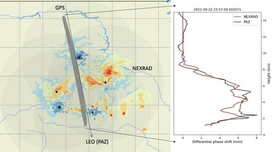
The Radio Occultacion (RO) technique, originally developed for planetary sciences to study other planets’ atmospheres (e.g., [1]), consists on tracking the signals emitted by a Global Positioning System (GPS) satellite from a Low Earth Orbit (LEO) satellite as it rises or sets behind the Earth’s limb. The technique measures the delay and bending caused by the refractivity of radio signals during propagation through the atmosphere. This delay can be utilized to derive radio refractivity profiles and ionospheric total electron content. From these radio refractivities, valuable vertical profiles of thermodynamic variables, including atmospheric pressure, temperature, and water vapor pressure, can be extracted from the stratosphere down to the surface with a vertical resolution ranging from 100 to 300 m (e.g., [2]). These products, derived from the standard RO technique, are currently assimilated operationally into various global Numerical Weather Prediction (NWP) models (e.g., [3]).
On 22 February 2018, the Spanish Earth Observation satellite PAZ was successfully launched, carrying a Global Navigation Satellite System (GNSS) Polarimetric Radio Occultation (PRO) payload. This mission, known as the Radio Occultation and Heavy Precipitation (ROHP) experiment, is led by the Institut de Ciéncies de l’Espai-Consejo Superior de Investigaciones Científicas/Institut de Estudis Espacials de Catalunya (ICE-CSIC/IEEC) in collaboration with NOAA, UCAR, and the NASA/Jet Propulsion Laboratory. The novelty of the PAZ mission lies in the acquisition of RO measurements at two linear polarizations for the first time [4].
The primary objective of the PRO technique is to detect heavy precipitation by measuring the difference in the phase delay between the two polarizations, horizontal (H) and vertical (V), of the GPS signals. Operating at L-band frequencies (L1 at 1.57542 GHz; L2 at 1.22760 GHz), these signals propagate through the atmosphere and reach the LEO satellite, which in the case of PAZ is equipped with a modified Integrated GPS Occultation Receiver (IGOR+) advanced GPS receiver [4]. The measurements of H and V polarizations are conducted independently, yet synchronously, employing a dual linearly polarized antenna directed towards the Earth’s limb in the anti-velocity direction of the LEO satellite. As the signals traverse deeper into denser atmospheric layers, they experience bending curvature induced by the refractive index vertical gradients. By acquiring the incoming electromagnetic field at the two linear and orthogonal polarizations, valuable information can be extracted concerning targets that introduce a differential phase shift () between the H and V components of the propagating signals. These targets are primarily hydrometeors that undergo flattening due to air drag during their descent or that are naturally asymmetric (e.g., snowflakes, graupel, etc.). In the presence of heavy precipitation events, the large droplets stand out for being oblate–spheroid-like. Therefore, the PRO technique offers the additional benefit of inferring vertical information about precipitation, enabling the retrieval of both the standard thermodynamic state of the surrounding area and vertical precipitation information within the same measurement.
The validation of the observable with two-dimensional data has been assessed in a statistical way using merged precipitation products like the Integrated Multi-satellitE Retrievals for GPM (IMERG) (e.g., [5,6]). Additionally, passive microwave radiometers have been used to help with the interpretation of the vertical structure [7], but these also provide limited vertical resolution retrievals. Furthermore, coincidences with the GPM Dual frequency Precipitation Radar (DPR) are sparse due to the limited swath of the space-based radar.
The initial hypothesis of the ROHP experiment, namely, that PRO observations are sensitive to heavy precipitation, was already demonstrated [5]. Furthermore, it has also been shown that the PRO observable increases with higher precipitation rain rates, indicating also sensitivity to precipitation intensity. Moreover, subsequent studies have shown that PRO is not only sensitive to precipitation, but also to horizontally oriented frozen hydrometeors found in various vertical layers of convective clouds [8,9]. This sensitivity is particularly pronounced for snow, where aggregated ice crystals produce relatively large hydrometeor particles. The combined sensitivity of PRO to both heavy precipitation and the associated cloud structures, along with its inherent capacity to provide colocated thermodynamic profiles, makes the PRO technique highly advantageous for studying heavy precipitation events. Other space-based observing systems focused on obtaining vertical thermodynamic profiles often have lower vertical resolution and encounter challenges when attempting measurements within deep clouds (e.g., [10]). On the other hand, space-based precipitation radars lack the capability to provide information about the thermodynamics. Overall, the demonstrated capabilities of PRO render it an interesting choice for investigating heavy precipitation phenomena, and the microphysics underlying these events.
Given that prior validations relied on two-dimensional data, this study seeks to enhance validation by employing three-dimensional data. The specific focus is on validating the vertical structure, and this can be achieved with the Next Generation Weather Radars (NEXRAD) dataset. This entails comparing the observable retrieved from PAZ with the vertical structures of derived from NEXRAD, which will permit us to calculate the equivalent differential phase shift observable from these radars.
This article is distributed as follows: Section 2 describes the data used in the analysis in order to make the comparison between NEXRAD and PAZ, and it also explains the methodology that has been followed; Section 3 shows the results of such comparison and the corresponding statistical analysis; finally, Section 4 accounts for the conclusions.
2. Materials and Methods
2.1. Polarimetric Radio Occultation Data
As it was already mentioned, the PRO technique allows us to compare the phase delay () associated with the two measured polarizations. Since situations of heavy precipitation are characterized by large horizontally oriented raindrops, the accumulated differential phase shift in these regions, , will be positive due to the depolarization effect [8]. takes a value of when the polarization is purely circular, and therefore, we will analyze with respect to the value it would have if the received field was purely circular: . More specifically, the registered in both ports of PAZ’s antenna contains the following terms:
where represents the carrier frequency, is the signature of the phase related to changes in the range between the transmitter and receiver, denotes the signatures of the phase due to atmospheric effects in the p-polarization (where p can be H or V), and indicates the signatures in the p-polarization phase induced by instrumental and platform environment effects [4].
As the first two terms in Equation (1) are independent of polarization, they cancel out when obtaining :
where should remain constant with time if no differential shift is introduced across the ray path. The instrumental term, , can be corrected with calibration [6]. Detailed theoretical analysis of other systematic effects can be found in [11].
The specific contribution to at each point of the propagation path is defined as the specific differential phase, . The values of are expressed in units of length (mm-shift/km-rain) instead of radians because these are the general units used in the GNSS community [4], and that is why it is multiplied by . The expression is the following:
where the wavelength, , corresponds to the GNSS; represents the real part; and are the forward scattering amplitudes describing the effect of scattering of the GNSS propagating waves by hydrometeors for the horizontal and vertical components, respectively; the variable D refers to the equivalent diameter of the drops; and is the particle size distribution (PSD). The terms accounting for the type of particle (liquid or solid) and its shape are the scattering amplitudes.
The total hydrometeors’ contribution along the ray path is therefore described by the following expression:
where the units of are in , is formulated in Equation (3), and L is the ray path length. As we deduce from Equation (4), there is an intrinsic ambiguity between the extension, L, and the intensity, in the final measurement.
The Calibrated PRO profiles from PAZ are available from May 2018 to the present [12]. Each file represents a PAZ observation and contains the vertical profile of the observable differential phase shift, , expressed in units of length (mm) and in terms of the tangential height of each PRO ray. As the PRO rays traverse the atmosphere from GPS to LEO, they bend due to refractivity gradients, eventually becoming tangential to the surface at their lowest height point, defined as the tangent point of the ray, . The locations (i.e., latitude and longitude) representative of each PRO observation are defined at the tangent point of the ray with = 4 km. Even though each ray is linked to its tangential height, hydrometeors that potentially present along the points in that ray are contributing to the value of , regardless of its height.
The PRO files also contain the locations (latitude, longitude and height) of each ray trajectory between the GPS and PAZ, obtained through ray-tracing techniques. These ray-path locations are calculated and re-gridded, so that only rays whose tangent height coincides with a regular grid between 0 and 20 km with a vertical resolution of 0.1 km are provided. This ensures a collection of ray trajectories with the same vertical resolution as , and that represent the trajectories that contribute to each measurement. Only the portion of these trajectories traveling below 20 km from the surface are considered, since it is assumed that no clouds nor hydrometeors are present above those heights.
2.2. NEXRAD Data
NEXRAD is a 160 network of dual-polarized weather radars distributed across the United States (US) and its territories, developed and deployed by the National Weather Service (NWS) of the US. NEXRAD radars operate at S-band (2–4 GHz) and their main advantage is that they are equipped with polarimetric capabilities, enabling them to provide valuable data on precipitation characteristics, such as size, shape and type of hydrometeor present in the atmosphere. These data are crucial for understanding severe weather phenomena like thunderstorms, tornadoes and heavy rainfall events. Additionally, dual-polarization allows for better discrimination between different types of precipitation, aiding in the identification of potential hazards. With a wide coverage across the US territory, NEXRAD radars offer real-time, high-resolution imagery of atmospheric conditions. The radars scan the sky in a 360-degree rotation, providing continuous updates on weather patterns, storm movements, and the evolution of weather systems. For more information about NEXRAD, see [13,14].
The NEXRAD data used here are obtained from the NEXRAD Level II dataset [15]. Each NEXRAD file contains fields for various variables, such as reflectivity (Z), differential reflectivity (), total differential phase (), cross-correlation ratio (), among others. These fields are provided as a function of azimuth, range, and elevation angle. For each radar, a 3D file is generated approximately every 8 min.
Typically, the radar scans have a range of elevation angles between 0.5° and 19.5°. Different variables have a different spatial resolution. For example, Z is provided at 1.0° azimuthal resolution and 1 km in range gate resolution, to a range of 460 km. Doppler velocity and spectrum width are provided at 1.0° azimuthal and 0.25 km in range gate resolution, to a range of 300 km.
2.3. Coincident Observations between PAZ and NEXRAD
The PAZ satellite is providing around 150/200 occultations per day, globally distributed, that pass quality control (QC). In the process of selecting the coincident observations, we have implemented a filtering criterion that includes all observations within a range of 250 km to a NEXRAD radar. The total number of observations between May 2018 and December 2022 that meet the colocation criteria is 3208.
To achieve the objectives of this study, we have carefully selected coincident observations from PAZ satellite and NEXRAD weather radars, ensuring they are colocated in both space and time. The time difference between the occultation and the NEXRAD data does not exceed 8 min, as we select the closest radar file to each observation. Typically, an occultation lasts for about 2 min. In terms of spatial alignment, we have chosen multiple radars for each PAZ observation to ensure a good coverage of the area sensed by the PRO rays below 20 km. To select the appropriate radars for each observation, we calculate the distances between all points along the PRO ray trajectories and the radar locations. Radars that do not reach any ray point within 250 km are discarded. Furthermore, the percentage of ray points that have at least one radar within a distance of 250 km is computed and stored as the covered area of each PRO.
Figure 1 shows the coverage of the NEXRAD radars over the continental U.S., panel (a), and an example of one coincident PRO observation, panels (b) and (c). Specifically, Figure 1b,c represents the observation in 3D and 2D, respectively. In Figure 1c we see, in grey, the projection on the surface of the portion of PRO rays below 20 km. This area is not the same for all observations since the geometry of the rays when they propagate through the atmosphere from the GPS to the LEO satellite will depend on the relative movement of both satellites. Depending on this movement, the rays originating at different altitudes will present a different degree of vertical alignment [6]. As shown in the figure, it is discernible that the extensive spatial coverage results in a limited vertical alignment among these rays, which can also be appreciated in Figure 1b.
2.4. Calculation of and from NEXRAD
To obtain vertical profiles of the observable using NEXRAD data, it is essential to calculate the variable since it is not directly provided in the NEXRAD Level II files. To accomplish this task and process the radar files, we use the Py-Art python module [16]. Once the radars for each observation are selected, the variable is calculated for each one of them. After evaluating various algorithms, we have found that the method described in [17,18] suits our purposes best, providing appropriate values of .
The algorithm in question, as well as the majority of algorithms subjected to testing, have been explained and compared in a prior publication, as documented in [19]. This specific algorithm that we use consists on a four-step process for retrieving the , and also allows us to adjust certain input parameters. These parameters are the number of iterations of the four step process, the dimensions of the sliding window employed in the smoothing, and a pre-filter procedure applied to the variable representing the total differential phase shift (), defined as:
being the differential phase shift measured by the radar and the differential backscatter phase shift.
Regarding the number of iterations, it has been empirically ascertained that variations therein do not yield a discernible impact on the final value of ; consequently, the default value of 10 iterations has been retained. The window size is defined as the extent of the sliding window employed for smoothing the before the calculation. As outlined in [19], smaller window sizes are better suited for scenarios featuring substantial values and steep gradients in , whereas larger window sizes are more appropriate for those characterized by gradual gradients in such variables. In the present study, it has been observed that the final profile undergoes significant variations in response to alterations in this parameter. To establish an optimal fit for the outcomes, a comprehensive analysis of the window size has been undertaken, with detailed findings presented in the subsequent section.
The pre-filter process applied to the raw values encompasses several steps, namely: the exclusion of values characterized by a correlation coefficient () below a specified threshold, herein set at 0.65; the identification and removal of portions marked by pronounced discontinuities; the elimination of exceedingly brief sequences of valid data; and the application of a median filter to each profile, as documented in [16]. The obtained from this algorithm is also corrected in terms of the elevation angle. This correction is essentially carried out due to the differences in the geometry of both techniques that we aim to compare. While in NEXRAD the signals exhibit a difference in the angle of incidence as the elevation emission angle from the radar changes, in PRO, the signals are practically tangential to the surface, meaning that the corresponding elevation angle is very close to 0 degrees. The correction is expressed by the following expression [20]:
where is the elevation angle, is the specific differential phase shift at an elevation angle of = 0°, and is the specific differential phase shift at an elevation angle .
The next step is to map the values obtained from NEXRAD to the PRO rays. To do so, we perform the interpolation with each of the selected radars for each PRO event, and calculate the mean of total overlapping interpolations. Through this process, we obtain the values corresponding to the radars for each PRO ray, measured in units of degrees per kilometer. Integrating the from NEXRAD along each PRO ray directly yields the at the S-band for each of the rays, which are associated with a specific tangential height . Finally, two conversions are performed to obtain the final profile: one to convert the units from degrees to millimeters and the other to transition from S-band to L-band. Considering that both bands are within the Rayleigh regime, the approximation made is a conversion factor [21]:
where represents the wavelength, and the subscripts S and L refer to the frequency bands. The first conversion term accounts for the conversion from S to L band, while the second term refers to the conversion from degrees to millimeters.
A smoothing process is also applied to the resulting vertical profile of , which uses a sliding window of five adjacent elements, with the aim of mitigating noise and accentuating the general trends within the profiles. Figure 2 shows an scheme of the steps followed in order to obtain the .
3. Results and Discussions
3.1. Sensitivity of to Window Size
To ascertain the optimal window size that suited our specific cases, we systematically assessed three distinct window dimensions, specifically, 4, 6, and 8. This parameter is expressed in units of number of gates, thus meaning that 4, 6, and 8 represent the number of gates we are considering for a specific window. Here, gate refers to a longitudinal element within the radar beam, representing a discrete volume of space. The length of one gate depends on the configuration at which the radar is operating. However, typically, the value of one gate is around km. The window size has to be an even number according to the algorithm specifications that we are using for retrieving . The three different window sizes were employed to perform the analysis in which we compute the vertical profiles of for each PAZ observation within our subset of coincidences. We have started by evaluating the correlation coefficient between the PAZ observations and the profiles derived from NEXRAD for these three window sizes, thereby facilitating the identification of the most appropriate window size for a particular observation.
The computation of the correlation coefficient was restricted to the altitude range spanning from km to 12 km to avoid low-altitude ambiguities in the PAZ retrievals [6]. On the other hand, an upper boundary was established as a safeguard measurement, prompted by the fact that when we reach the altitude at which no targets are detected the values of the NEXRAD profiles asymptotically approach zero, whereas the PAZ data continues to exhibit small fluctuations due to noise. This upper threshold was imposed to ensure that this disparity does not influence the correlation coefficient.
In an analogue way, observations where we do not have precipitation are characterized by a vertical profile of that is completely or almost completely zero, and a vertical profile of that contains some noise. For this reason, the correlation coefficient that we will have associated with non-rain events will be practically zero. Therefore, in Figure 3, we present the correlation coefficient values computed exclusively for cases that involve rain events. This selection process encompasses isolating cases from the dataset of PAZ-NEXRAD coincidences based on specific criteria: we considered cases where the mean value from PAZ, between 0 and 10 km, exceeded mm and where radar coverage of the PRO area exceeded . We have also discarded four cases where the had unrealistic values.
The analysis reveals that, except for two (three) cases when employing a window size of 4 (6) gates, most PAZ observations demonstrate a notable concordance with the corresponding profiles of . These three cases that exhibit a lack of correlation in the profiles appear to manifest anomalous data retrieval issues within the NEXRAD radar system. We also have a larger amount of cases that fit the previous restrictions for the window size of four gates.
While the correlation coefficient provides an indication on the agreement about the shape of the vertical profiles, computing the mean values of the between two heights provide further indication on the agreement between the magnitudes. The mean between 2 km and 8 km for PAZ and NEXRAD has been computed for the profiles obtained with the three window sizes, and the results of the comparison between the two are shown in Figure 4. When no or little precipitation is observed (small values of ), it can be seen how there is larger dispersion in the when the window size is smaller. This was the same result as obtained in [19], where they have seen that smaller window sizes performed better for larger values of , while larger window sizes did for smaller values of . This is mainly because smaller values of are typically associated to the presence of small raindrops or drizzle, and therefore, employing a larger window size could help reduce excessive noise and average the small-scale variations and provide a smoother representation. Whereas when measuring higher values of , there may be more pronounced variations over shorter distances so a smaller window size might be preferred in order to capture these variations at a finer spatial scale.
Similarly, it is observed that for larger values of , there exists an inverse proportionality with respect to the window size on the , where smaller window sizes are associated with larger values of . This is expected due to the fact that smaller window sizes in the smoothing of the observations allow for rapidly varying regions to be inverted to , which could correspond to noisy observations or areas of precipitation.
All in all, the results in Figure 4 indicate that, for the majority of cases, the and agree better for small window sizes in large regimes, while the agreement is better using a larger window size under low conditions. This suggests that an adaptative window size to specific precipitation regimes would be a good idea, as has been previously suggested in [22]. This, however, is not implemented in the Py-Art retrievals and is out of the scope of this work to perform such modifications.
Continuing with the analysis, we have also examined situations in which there is no precipitation. Since the correlation coefficient would not be a representative value of the agreement between both profiles, based on what we have already commented, we show the histograms present in Figure 5a,b. In Figure 5a, we have selected, for various window sizes, those cases in which the mean of below 10 km is less than 1 mm. For these observations, we have plotted the histogram of corresponding values of the mean below 10 km and calculated the percentage of these observations with a mm. The analogue has been represented in Figure 5b where the values of the mean are represented for those observations with a mean mm. From the results depicted in Figure 5a,b, it is observed that for both figures and various window sizes, over 85% of the cases exhibit values below 1 mm. This agrees with the fact that the noise values considered for this observable are less than 1.5 mm as stated in [5,6]. This implies that for most observations where PAZ does not detect rainfall, the NEXRAD radars do not detect precipitation either.
Table 1 shows the number of colocated observations that we have depending on the restrictions that we apply.
We should also take into consideration that we are using the radar data that is temporally closest to the observations. Radar data are generated approximately every 8 min, and the time we consider as the PAZ observation time is the start of the occultation, which lasts for approximately 2 min. Hence, in situations involving rapidly evolving precipitation events, there may be an associated error that warrants careful consideration. Furthermore, it is possible that there are situations in which a significant portion of the precipitation is not covered by the radar observations. The selection of the 60% area coverage threshold was made with the aim of ensuring an adequate number of cases for statistical analysis while also ensuring that a substantial portion of the occultation area is covered.
3.2. Illustrative Examples of Vertical Profiles of
The main aim of this investigation is to assess the agreement between vertical profiles of obtained from PAZ and from NEXRAD. As demonstrated in Figure 3 and Figure 4, the agreement for well-covered, precipitating cases is good. Furthermore, in this section we scrutinize three specific cases of coincident observations between PAZ and NEXRAD, where PRO rays intersect precipitation regions (see Figure 6, Figure 7 and Figure 8). Through a meticulous side-by-side comparison, our goal is to identify significant similarities or differences in the measurements obtained by both instruments during precipitation events. In addition, we present a statistical analysis of the difference between and to provide a broader and more comprehensive perspective on the results.
Upon examination of these profiles, a noteworthy degree of similarity becomes evident. The absence of values at lower altitudes is intentional to mitigate ambiguities in the PAZ profiles at those heights. Nevertheless, in all cases, both the shape and magnitude of the profiles exhibit a high degree of concordance. While most peaks are consistently represented in both profiles, they may not align precisely in terms of altitude. Discrepancies in the profiles may be attributed, in part, to factors such as instrumental characteristics, variations in measurement methodology, time differences in the case of rapidly evolving precipitation, and retrieval errors.
Moreover, a substantial presence of hydrometeors at lower altitudes (around 2–4 km, as observed in Figure 6 and Figure 7) corresponds to a higher level of agreement between PAZ and NEXRAD profiles, in terms of the shape of the profile. Conversely, for peaks situated at higher altitudes (approximately 5–7 km, as is seen in the case shown in Figure 8), the agreement diminishes. This reduction may be attributed to the potential influence of mixed-phase hydrometeors around these altitudes and also to the presence of smaller particles that are more difficult to be sensed by PAZ because of the lower frequency employed. A window size of 4 gates was employed for the three cases presented here. However, while our analysis indicates that a window size of 4 gates yields a superior correlation coefficient for the majority of cases, observations exist where an alternative window size demonstrates a better fit. This variation emphasizes the importance of customizing the analysis to specific cases in order to ensure the most accurate results when calculating .
3.3. Statistical Analysis of Differences
From a broader perspective, statistics on the difference between and for all cases fulfilling the coverage condition (i.e., coverage > 60%) have been computed. The outcomes of this analysis are depicted in Figure 9. Each column in the figure corresponds to a different window size, while each row imposes a distinct constraint on the mean within the altitude range of 0–10 km. The first row illustrates scenarios where mm (associated to heavy precipitation regime), the second row comprises observations with mm (linked to lower precipitation regimes), and the third row includes colocated cases in which PAZ has not detected precipitation, denoted by mm.
In Figure 9a–c, corresponding to the heavier precipitation regime, the discernible trend reveals an increasing positivity in the median difference between from PAZ and NEXRAD with the increase of the window size. This observation aligns with expectations, as commented earlier, where the values of exhibit a diminishing trend with an increasing window size. Notably, the optimal window size appears to be for 6 gates, a choice supported to some extent by favorable outcomes in Figure 3 and Figure 4 when employing this size for the moving window. Nevertheless, at altitudes spanning 6–8 km, the window size of 4 gates seems to be a potentially better choice, again revealing discrepancies in regions characterized by a higher concentration of mixed-phase hydrometeors and possibly by smaller hydrometeors.
For Figure 9d–f, corresponding to lighter precipitation than the previous case, a similar pattern is observed, with the difference between PAZ and NEXRAD exhibiting an increasing positivity correlated with the window size. However, here the optimal window size is inferred to be 8 gates, a fact consistent with the previous comments that a larger window size is preferable for scenarios with lower values of .
Figure 9g–i depict the statistics for cases with no or very little precipitation, where the difference remains practically invariant across the different window sizes. For this cases, where values from NEXRAD are expected to be near 0, the result of the difference between and is expected to yield values consistent with the PAZ noise. The results presented here resemble those obtained in [6], with small standard deviations of increasing with decreasing altitude.
In summary, for instances where precipitation has been identified, the importance of the selected window size becomes relevant in ensuring accurate determinations of . Throughout this analysis, the same window size has been applied uniformly across all radars surrounding an observation. Nevertheless, it warrants consideration to investigate whether better results could be achieved by adapting the window size based on the specific precipitation characteristics encountered along each radar ray. Such an approach may offer valuable insights into optimizing the accuracy and relevance of estimations.
3.4. Echotop Height Comparison
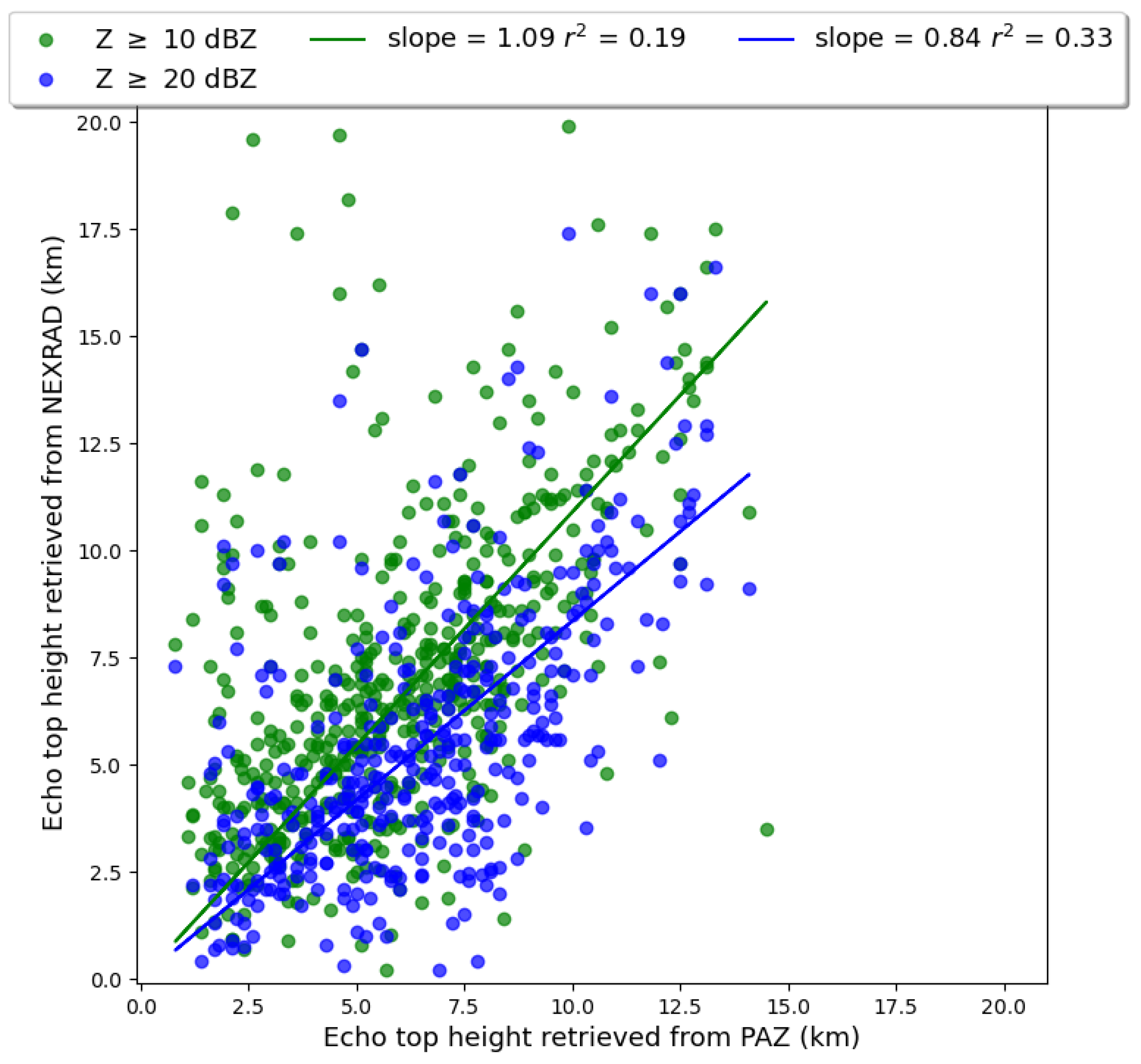
A final study of the concordance between and has been performed, consisting on comparing the echotop height values extracted from both datasets, as depicted in Figure 10. The determination of NEXRAD’s echotop consists on the interpolation of reflectivity data from the radars onto the PRO rays, analogous to the approach applied to . The following thresholds were applied to the reflectivity values: dBZ and dBZ. By identifying the maximum height associated with these thresholds, we then select the associated tangential height of the ray that actually crosses that point, instead of the actual height. By doing this, we are not obtaining the “real” echotop height but the “projected” one to the tangent point, and this is done to ensure a fair comparison between the two observational techniques.
The echotop equivalent for PAZ observations was defined as the highest point where surpasses a threshold for five consecutive measurements. This threshold was calculated by taking the mean of values above 20 km (where neither rain nor clouds are anticipated) and adding four times the standard deviation. This rigorous criterion ensures that if surpassed, the signature unequivocally originates from precipitation or cloud-related effects.
Figure 10 shows roughly a linear relationship between the two, with exceptions attributable to cases where precipitation was not detected. This can be appreciated by the values of the slope for the linear regression, being the one corresponding to dBZ the closest to one. For the case where dBZ, it is evident that “echotop” heights recorded by PAZ are lower than those of NEXRAD. This suggests that PAZ underestimates the echotop height compared to NEXRAD, registering lower upper boundaries of the precipitation layers. These differences could be attributed to factors such as respective frequencies employed by each instrument for detection, being NEXRAD more sensitive to smaller particles than PAZ. This may indicate that the specific hydrometeors associated with such thresholds are smaller than what PAZ can effectively detect. Besides, the instruments could be more sensitive to different atmospheric layers. NEXRAD is more sensitive to smaller particles, so they might be detecting features in a higher atmospheric layer than PAZ.
4. Conclusions
In this study, we have selected colocated observations from the PAZ satellite and NEXRAD ground-based radars in order to validate the vertical structure of the PRO observable. Such validation is achieved by using NEXRAD to obtain profiles of differential phase shift. These profiles were then subjected to a comparative analysis against their analogues retrieved from PAZ. Furthermore, an investigation focused on optimizing the smoothing window parameter for calculating the variable was conducted with the aim of achieving the best fit between the profiles. Subsequently, both the distinctions and similarities within these profiles were discussed, and some properties were subject to individual examination. It has been shown that the agreement holds for both the shape and magnitude of the observable. Moreover, statistical comparison using selected profiles grouped by different precipitation regimes exhibit mean differences and dispersion consistent with the used window size; that is, agreement increases with lower window size when considering heavier precipitation, whereas the agreement is better using larger window size when precipitation is lighter. Also, for the non-rainy cases, the are no significant biases, and the dispersion agrees with that reported in previous studies.
The good agreement observed between the vertical profiles obtained from both platforms show the potential of PAZ PRO observations in characterizing, to some extent, the vertical structure of heavy precipitation events. This underscores the potential for multi-platform validation of precipitation measurements, particularly in regions with limited ground-based radar coverage. Besides, it makes clear the PAZ mission’s capabilities to contribute to heavy precipitation research, emphasizing the method’s importance as a powerful tool for further enhancing the understanding and characterization of precipitation events and their associated thermodynamics.
Notably, we have identified remarkable consistency in the detection altitudes of hydrometeors between PAZ and NEXRAD, with numerous observations showing that both instruments identify hydrometeors at similar altitudes. However, some differences were observed under specific meteorological conditions, particularly around altitudes where the presence of small frozen particles is more pronounced. Due to the higher frequency employed by NEXRAD compared to PAZ, the radars are more sensitive to such small particles. This sensitivity leads to variations in detection altitudes for specific hydrometeor types. Nevertheless, PAZ observations demonstrate increased sensitivity to particles such as snow. This is thought to be due to the geometry employed by the technique. Therefore, the combination of data from PAZ and NEXRAD could enhance our ability to interpret radar data in regions experiencing mixed-phase precipitation.
It is imperative to acknowledge that certain observed disparities may be attributed to factors such as instrumental characteristics and variations in measurement methodologies, as well as retrieval errors. Consequently, a prudent consideration of these limitations is essential when drawing conclusions from this study. Besides, radar-based data are subject to some uncertainties such as anomalous propagation, partial beam filling, beam overshooting and spatio-temporal resolution, among others.
Also, it is worth mentioning that we encountered certain challenges in processing NEXRAD Level II data. Two of the algorithms mentioned in [19] were impractical to apply due to their computational cost, and another provided values lacking physical significance. Regarding the window size, existing literature on the optimal choices based on radar-derived variable values was limited, as was the guidance for selecting a specific window size for a particular case study. Since the is a polarimetric variable independent of attenuation and miscalibration, it is a valuable variable for many analyses, so in regard to the different processes to calculate , the data obtained from PAZ could prove useful in refining this procedure.
In summary, this research solidifies the PRO technique as an instrument for quantifying heavy precipitation events. It emphasizes the role played by satellite-based systems, such as PAZ, in advancing our comprehension of hydrometeor detection and characterizing the microphysical properties of the atmosphere, especially in remote regions experiencing complex weather phenomena.
As for future work, there is potential to adapt the algorithm to consider variations in window size based on the polarimetric and non-polarimetric variables measured by the radar. We have seen in this study that some precipitation characteristics could be taken into consideration when selecting the proper window size. Additionally, exploring algorithms that classify hydrometeors could be valuable for a more in-depth study of areas with mixed-phase hydrometeors, providing insights into the sensitivity of to these conditions.
Author Contributions
Conceptualization, A.P., R.P. and E.C.; methodology, A.P.; software, A.P.; validation, A.P., R.P. and E.C.; formal analysis, A.P.; investigation, A.P, R.P. and E.C.; resources, E.C.; data curation, A.P.; writing—original draft preparation, A.P.; writing—review and editing, A.P., R.P. and E.C.; visualization, A.P.; supervision, R.P. and E.C.; project administration, E.C.; funding acquisition, E.C. All authors have read and agreed to the published version of the manuscript.
Funding
The ROHP-PAZ project is part of the Grant PID2021-126436OB-C22 funded by the Spanish Ministry of Science and Innovation MCIN/AEI/10.13039/501100011033 and by “ERDF A way of making Europe” of the “European Union”. R.P is funded by the grant RYC2021-033309-I, included in the «NextGenerationEU»/PRTR. This work was also partially supported by the program Unidad de Excelencia María de Maeztu CEX2020-001058-M. Part of the investigations are done under the EUMETSAT ROM SAF CDOP4.
Data Availability Statement
Data from PAZ is available at: https://paz.ice.csic.es/ [12] (accessed on 18 March 2024). Level II data from NEXRAD is available at: https://s3.amazonaws.com/noaa-nexrad-level2/index.html [15] (accessed on 18 March 2024).
Acknowledgments
The authors would like to thank the developers of Py-Art for creating and making available this Python module to easily analyze data obtained from weather radars. We express our gratitude to three anonymous reviewers whose comments contributed to the improvement of the manuscript.
Conflicts of Interest
The authors declare no competing interests.
Abbreviations
The following abbreviations are used in this manuscript:
| GNSS | Global Navigation Satellite Systems |
| PRO | Polarimetric Radio Occultation |
| NEXRAD | Next Generation Weather Radars |
| ROHP | Radio Occultation and Heavy Precipitation |
| ICE-CSIC | Institut de Ciéncies de l’Espai-Consejo Superior de Investigaciones Científicas |
| IEEC | Institut d’Estudis Espacials de Catalunya |
| NOAA | National Oceanic and Atmospheric Administration |
| UCAR | University Corporation for Atmospheric Research |
| NASA | National Aeronautics and Space Administration |
| GPS | Global Positioning System |
| LEO | Low Earth Orbit |
| IGOR+ | Integrated GPS Occultation Receiver |
| NWP | Numerical Weather Prediction |
| GPM | Global Precipitation Mission |
| GMI | GPM Microwave Imager |
| PPI | Plan Position Indicator |
| PSD | Particle Size Distribution |
| IMERG | Integrates Multi-satellitE Retrievals for GPM |
| DPR | Dual frequency Precipitation Radar |
| NWS | National Weather Service |
| QC | Quality Control |
References
- Fjeldbo, G.; Eshleman, V.R. The Bistatic Radar-Occultation Method for the Study of Planetary Atmospheres. J. Geophys. Res. 1965, 70, 3217–3225. [Google Scholar] [CrossRef]
- Kursinski, E.R.; Hajj, G.A.; Schofield, J.T.; Linfield, R.P.; Hardy, K.R. Observing Earth’s atmopshere with radio occultation measurements using the Global Positioning System. J. Geophys. Res. Atmos. 1997, 102, 23429–23465. [Google Scholar] [CrossRef]
- Healy, S.B.; Jupp, A.M.; Marquardt, C. Forecast impact experiment with GPS radio occultation measurements. Geophys. Res. Lett. 2005, 32, L3804. [Google Scholar] [CrossRef]
- Cardellach, E.; Tomás, S.; Oliveras, S.; Padullés, R.; Rius, A.; de la Torre Juárez, M.; Turk, F.; Ao, C.; Kursinski, E.R.; Schreiner, B.; et al. Sensitivity of PAZ LEO Polarimetric GNSS Radio-Occultation Experiment to Precipitation Events. IEEE Trans. Geosci. Remote Sens. 2014, 53, 190–206. [Google Scholar] [CrossRef]
- Cardellach, E.; Oliveras, S.; Rius, A.; Tomás, S.; Ao, C.; Franklin, G.W.; Iijima, B.A.; Kuang, D.; Meehan, T.K.; Padullés, R.; et al. Sensing Heavy Precipitation With GNSS Polarimetric Radio Occultations. Geophys. Res. Lett. 2019, 46, 1024–1031. [Google Scholar] [CrossRef]
- Padullés, R.; Ao, C.; Turk, F.; de la Torre Juárez, M.; Iijima, B.; Wang, K.N.; Cardellach, E. Calibration and validation of the Polarimetric Radio Occultation and Heavy Precipitation experiment aboard the PAZ satellite. Atmos. Meas. Tech. 2020, 13, 1299–1313. [Google Scholar] [CrossRef]
- Turk, F.; Padullés, R.; Cardellach, E.; Ao, C.; Wang, K.N.; Morabito, D.D.; de la Torre Juárez, M.; Oyola, M.; Hristova-Veleva, S.; Neelin, J.D. Interpretation of the Precipitation Structure Contained in Polarimetric Radio Occultation Profiles Using Passive Microwave Satellite Observations. J. Atmos. Ocean. Technol. 2021, 38, 1727–1745. [Google Scholar] [CrossRef]
- Padullés, R.; Cardellach, E.; Turk, F.; Ao, C.; de la Torre Juárez, M.; Gong, J.; Wu, D.L. Sensing Horizontally Oriented Frozen Particles With Polarimetric Radio Occultations Aboard PAZ: Validation Using GMI Coincident Observations and Cloudsat a Priori Information. IEEE Trans. Geosci. Remote Sens. 2021, 60, 1–13. [Google Scholar] [CrossRef]
- Padullés, R.; Cardellach, E.; Turk, F. On the global relationship between polarimetric radio occultation differential phase shift and ice water conten. Atmos. Chem. Phys. 2023, 23, 2199–2214. [Google Scholar] [CrossRef]
- Wulfmeyer, V.; Hardesty, R.M.; Turner, D.D.; Behrendt, A.; Cadeddu, M.P.; Di Girolamo, P.; Schlüssel, P.; Baelen, J.V.; Zus, F. A review of the remote sensing of lower tropospheric thermodynamic profiles and its indispensable role for the understanding and the simulation of water and energy cycles. Rev. Geophys. 2015, 53, 819–895. [Google Scholar] [CrossRef]
- Tomás, S.; Padullés, R.; Cardellach, E. Separability of systematic effects in polarimetric GNSS radio occultations for precipitation sensing. IEEE Trans. Geosci. Remote Sens. 2018, 56, 4633–4649. [Google Scholar] [CrossRef]
- Padullés, R.; Cardellach, E.; Oliveras, S. resPrf [Dataset]. 2024. Available online: https://digital.csic.es/handle/10261/348253 (accessed on 18 March 2024).
- Klazura, G.E.; Imy, D.A. A Description of the Initial Set of Analysis Products Aivailable from the NEXRAD WSR-88D System. Bull. Am. Meteorol. Soc. 1993, 74, 1293–1312. [Google Scholar] [CrossRef]
- Crum, T.D.; Saffle, R.E.; Wilson, J.W. An Update on the NEXRAD Program and Future WSR-88D Support to Operations. Weather Forecast. 1998, 13, 253–262. [Google Scholar] [CrossRef]
- NOAA National Weather Service (NWS) Radar Operations Center. NOAA Next Generation Radar (NEXRAD) Level 2 Base Data; National Centers for Environmental Information: Asheville, NC, USA, 1991. [CrossRef]
- Helmus, J.J.; Collis, S.M. The Python ARM Radar Toolkit (Py-Art), a library for working with weather radar data in the Python programmin language. J. Open Res. Softw. 2016, 4, e25. [Google Scholar] [CrossRef]
- Vulpiani, G.; Montopoli, M.; Passeri, L.D.; Gioia, A.G.; Giordano, P.; Marzano, F.S. On the use of dual-polarized C-band radar for operational rainfall retrieval in mountainous areas. J. Appl. Meteorol. Climatol. 2012, 51, 405–425. [Google Scholar] [CrossRef]
- Vulpiani, G.; Baldini, L.; Roberto, N. Characterization of Meditarranean hail-bearing storms using an operational polarimetric X-band radar. Atmos. Meas. Tech. 2015, 8, 4681–4698. [Google Scholar] [CrossRef]
- Reimel, K.J.; Kumjian, M. Evaluation of Kdp Estimation Algorithm Performance in Rain Using a Known-Truth Framework. J. Atmos. Ocean. Technol. 2021, 38, 587–605. [Google Scholar] [CrossRef]
- Griffin, E.M.; Schuur, T.J.; Ryzhkov, A.V. A Polarimetric Analysis of Ice Microphysical Processes in Snow, Using Quasi-Vertical Profiles. J. Appl. Meteorol. Climatol. 2018, 57, 31–50. [Google Scholar] [CrossRef]
- Bringi, V.N.; Chandrasekar, V. Polarimetric Doppler Weather Radar: Principles and Applications; Cambridge University Press: Cambridge, UK, 2001. [Google Scholar]
- Wang, Y.; Chandrasekar, V. Algorithm for Estimation of the Specific Differential Phase. J. Atmos. Ocean. Technol. 2009, 26, 2565–2578. [Google Scholar] [CrossRef]
Figure 1.
In panel (a), the distribution of NEXRAD radar across the continental United States is shown. Black points indicate radar locations, with the blue areas illustrating the approximate range of the radars. The panel (b) showcases a particular colocated observation of PAZ and NEXRAD in 3D, while panel (c) shows the same observation in a 2D image. Only the portion of the rays below 20 km is shown. The gray region in panel (c) represents the 2D projection of the PRO rays, and the coloured map is a Plan Position Indicator (PPI) of the reflectivity measured by the selected radars for that observation.
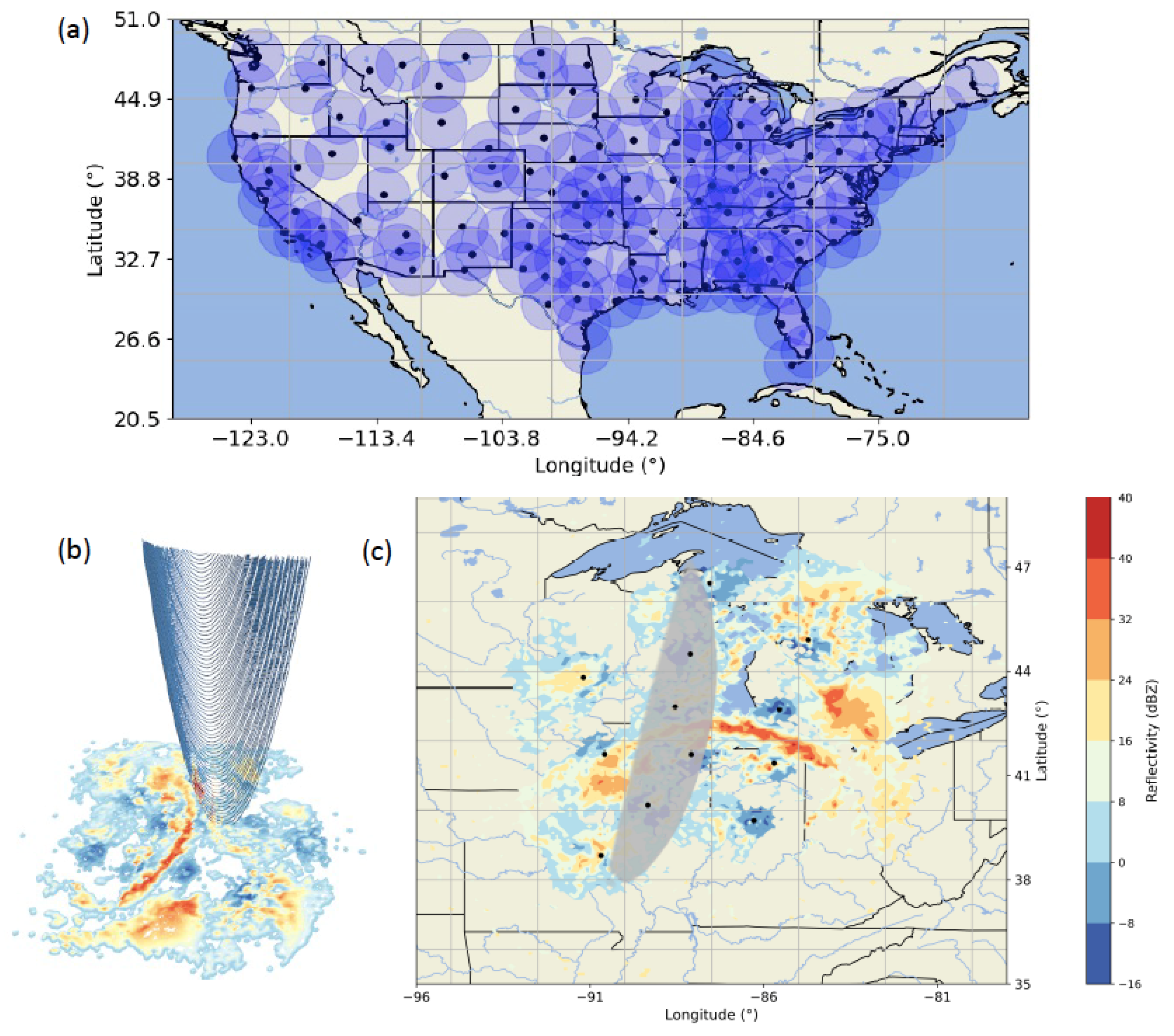
Figure 2.
Diagram showing the steps followed to obtain the vertical profiles of from NEXRAD.
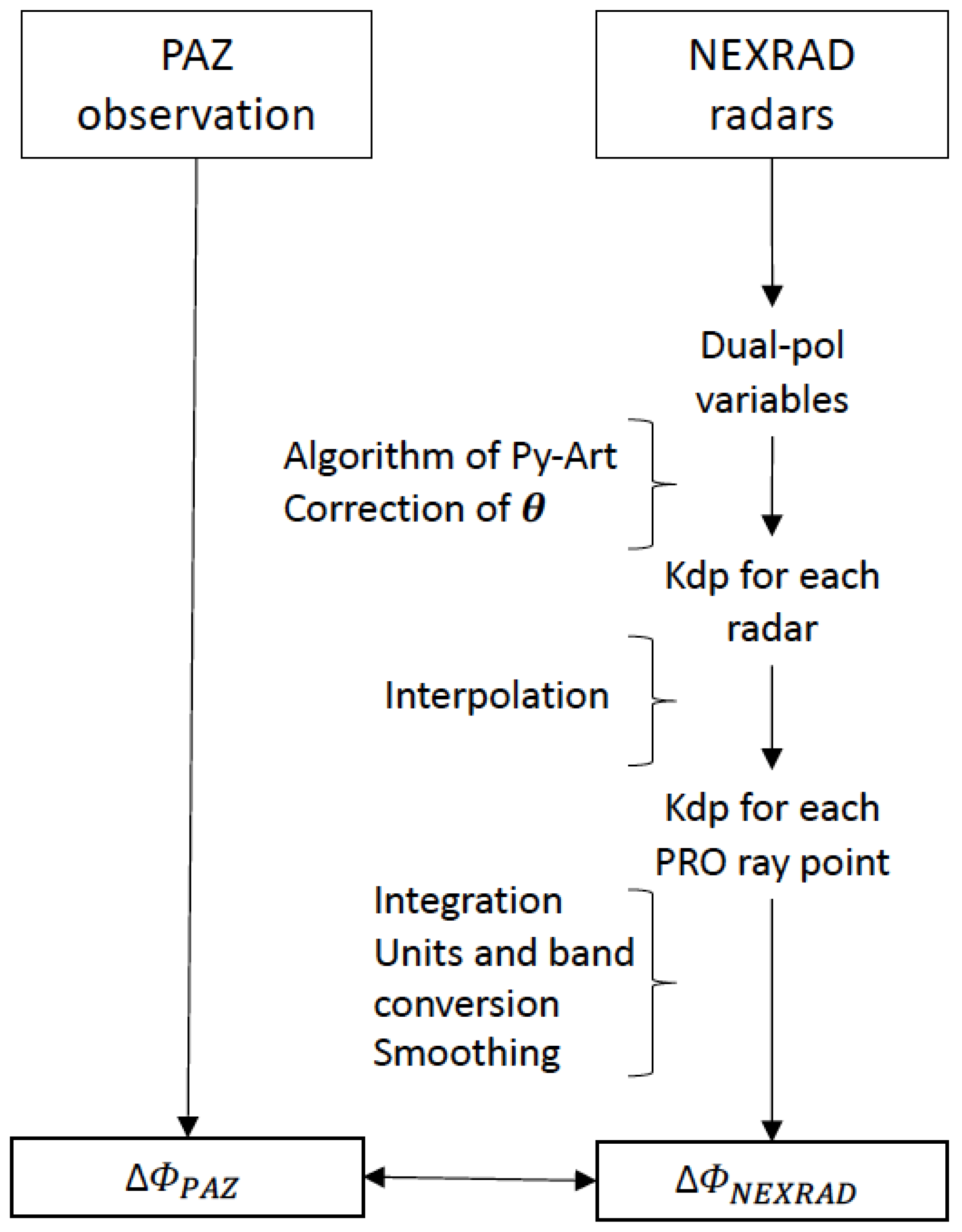
Figure 3.
Histogram showing the correlation coefficient for the cases considered as rainy events (see text), for the different window sizes represented in different colors (as indicated in the legend).
Figure 3.
Histogram showing the correlation coefficient for the cases considered as rainy events (see text), for the different window sizes represented in different colors (as indicated in the legend).
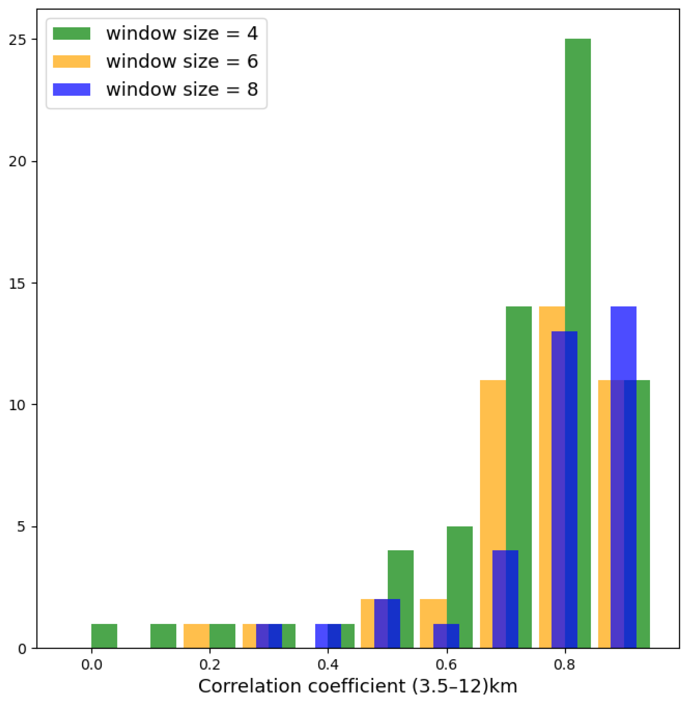
Figure 4.
Mean (mm) between 2 km and 8 km for both NEXRAD and PAZ and for three window sizes. The slope and the coefficient of determination are also displayed in the legend. The colocated observations presented here are the ones where the radar coverage exceeds 60%.
Figure 4.
Mean (mm) between 2 km and 8 km for both NEXRAD and PAZ and for three window sizes. The slope and the coefficient of determination are also displayed in the legend. The colocated observations presented here are the ones where the radar coverage exceeds 60%.
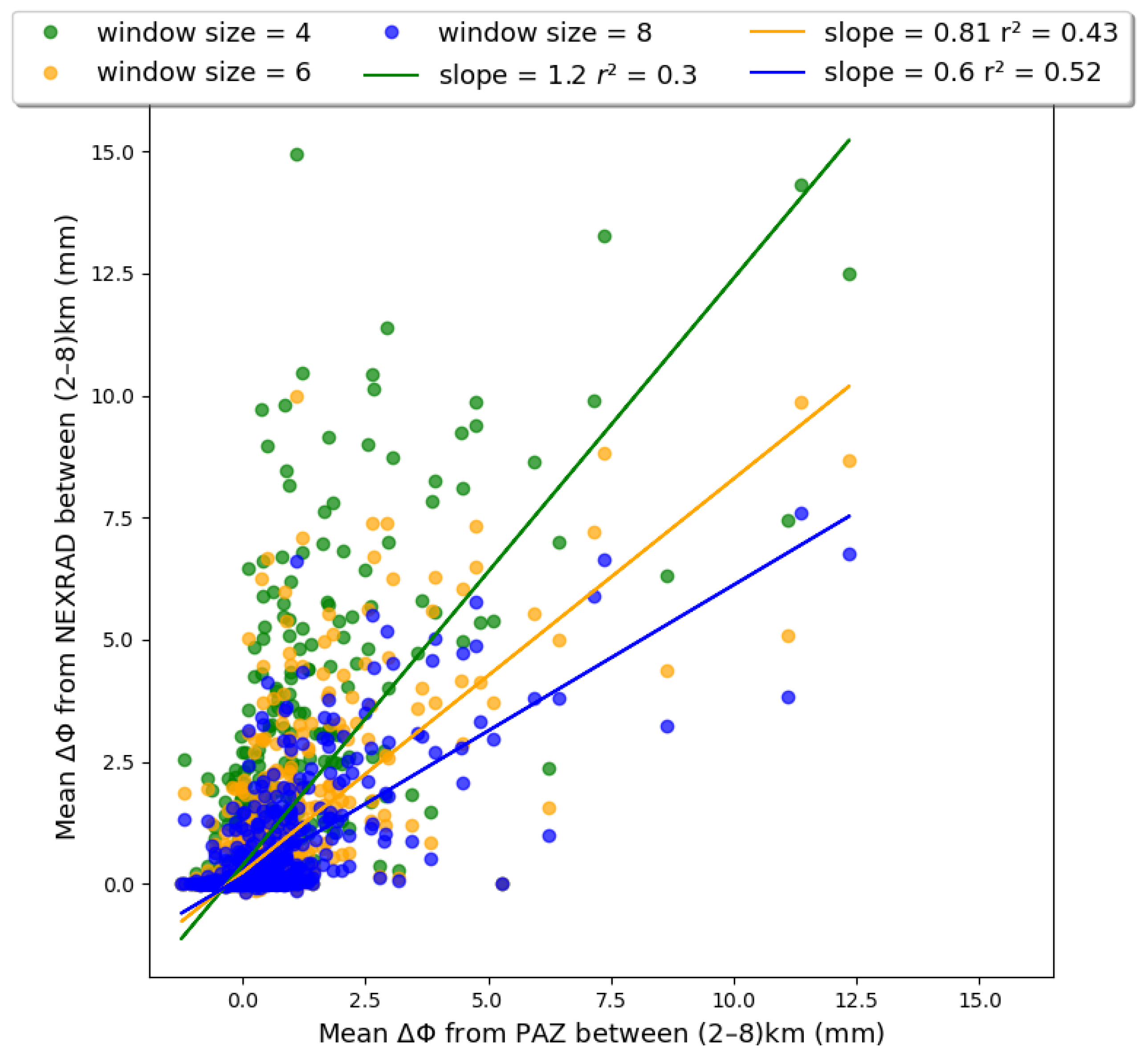
Figure 5.
Mean between 0–10 km (a) for those observations where the mean between 0–10 km is below 1 mm, and between 0–10 km (b) for those observations where the mean of between 0–10 km is below 1 mm. For each of the window sizes we have calculated the percentage of the cases that have the mean between 0–10 km below 1 mm (a) and between 0–10 km below 1 mm (b).
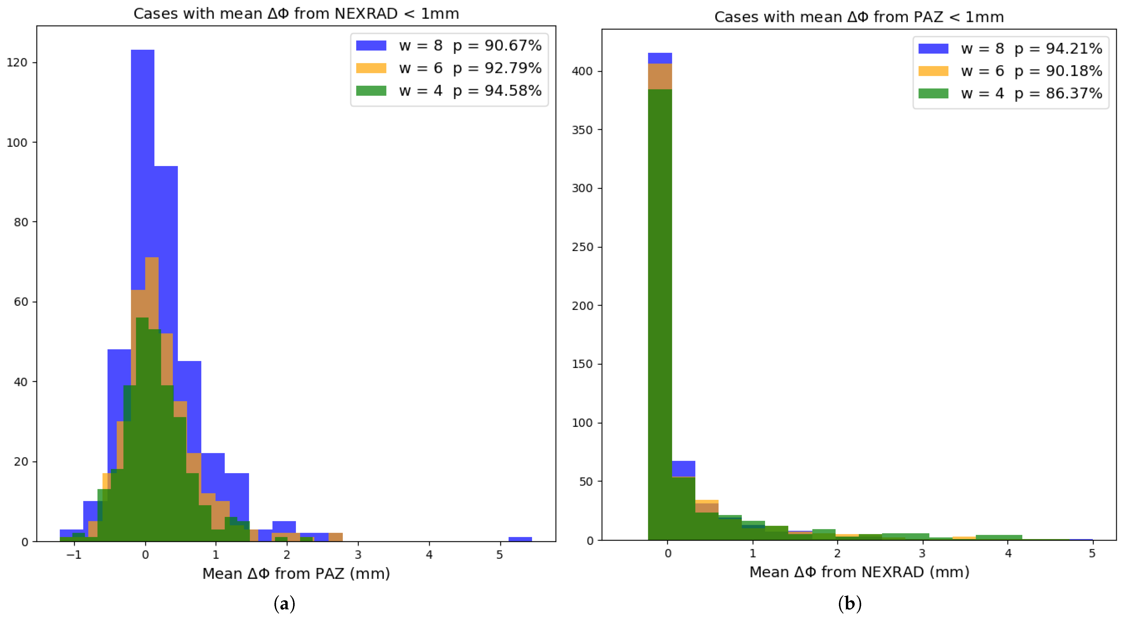
Figure 6.
PAZ observation (ID: PAZ1.2020.057.22.53.G09) colocated with NEXRAD radars and the associated vertical profiles for both instruments. The left panel shows the composite field captured by the radars (black points indicate radar locations) with the area of the projection on the surface of the portion of PRO rays below 20 km, in grey. Right panel shows the corresponding vertical profiles of as obtained using NEXRAD data (red) and PAZ (black). In the legend we also present the corresponding values of window size (w), the correlation coefficient (cc) and the percentage of the area covered by the radars (p).
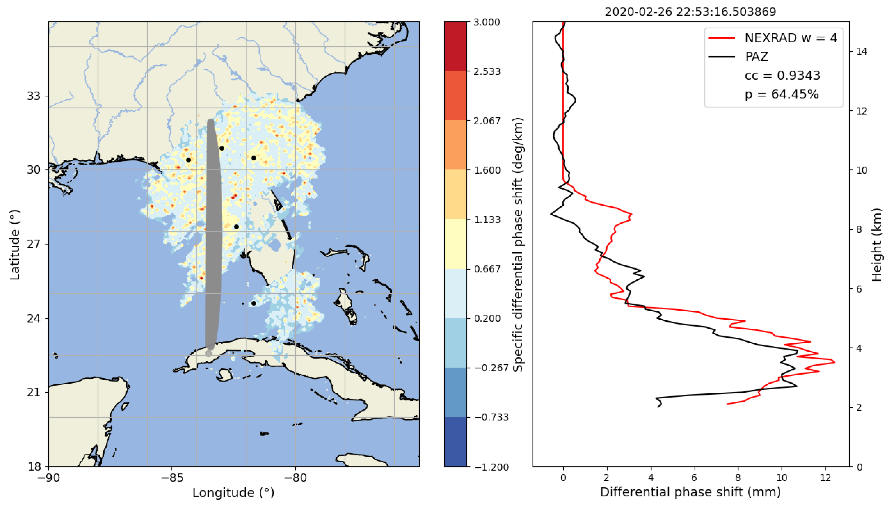
Figure 7.
Same as in Figure 6, but corresponding to PAZ profile ID PAZ1.2021.220.13.34.G01.
Figure 7.
Same as in Figure 6, but corresponding to PAZ profile ID PAZ1.2021.220.13.34.G01.
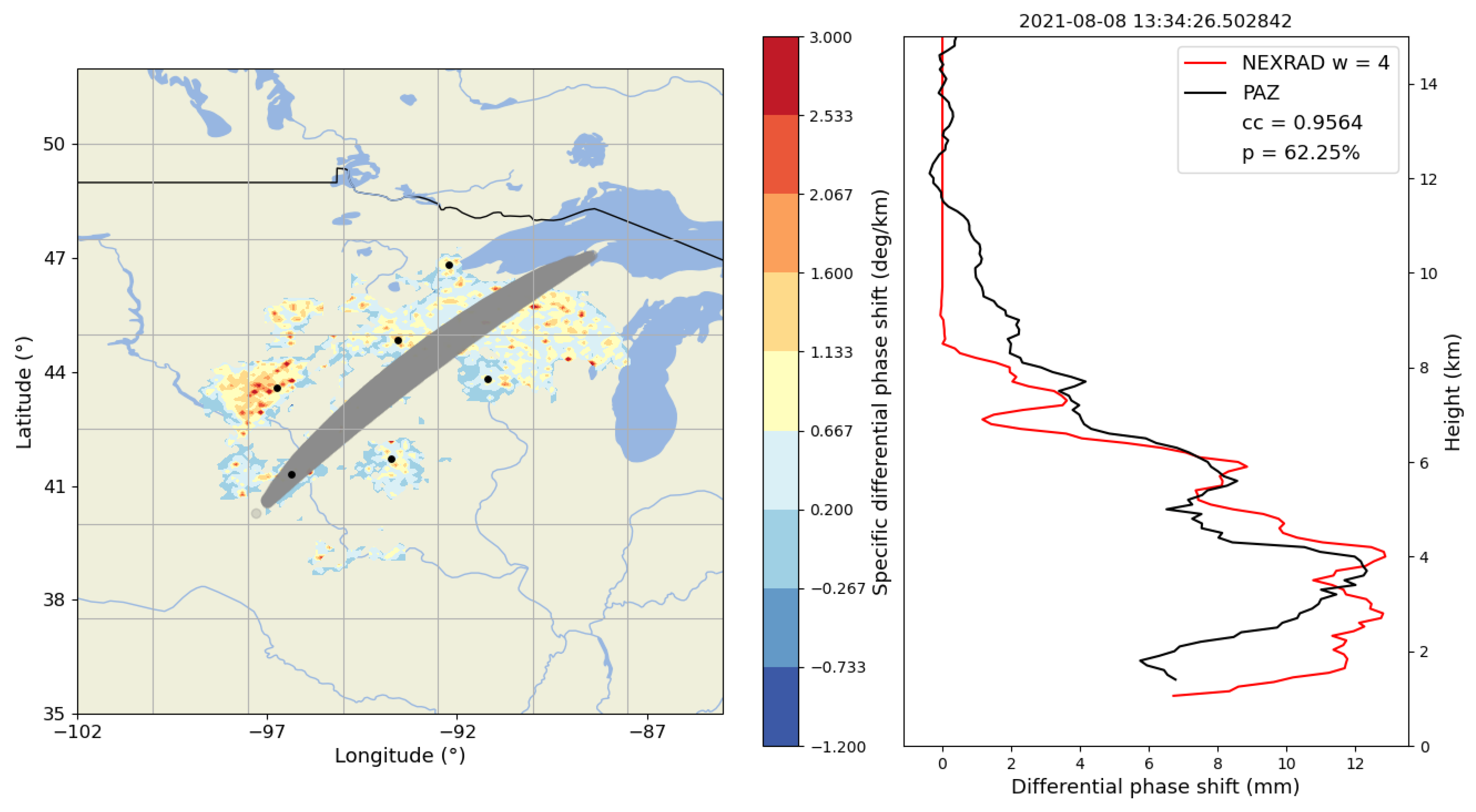
Figure 8.
Same as in Figure 6, but corresponding to PAZ profile ID PAZ1.2018.360.23.55.G11.
Figure 8.
Same as in Figure 6, but corresponding to PAZ profile ID PAZ1.2018.360.23.55.G11.

Figure 9.
Difference between and for those cases that are covered more than by the radars. Each column represents a different window size ((a,d,g) represent a window size = 4, etc.), while each row represents a different condition for the mean between 0–10 km. For the first row, the cases represented are the ones were PAZ has detected rain and is larger than 4 mm. In second row, we represent as well cases where PAZ has detected precipitation but is lower than 4mm. The third row represents those cases where PAZ has not detected precipitation, this means that is between ±0.5 mm. For each figure the number of valid points for each altitude is represented by a red line (top x-axis).
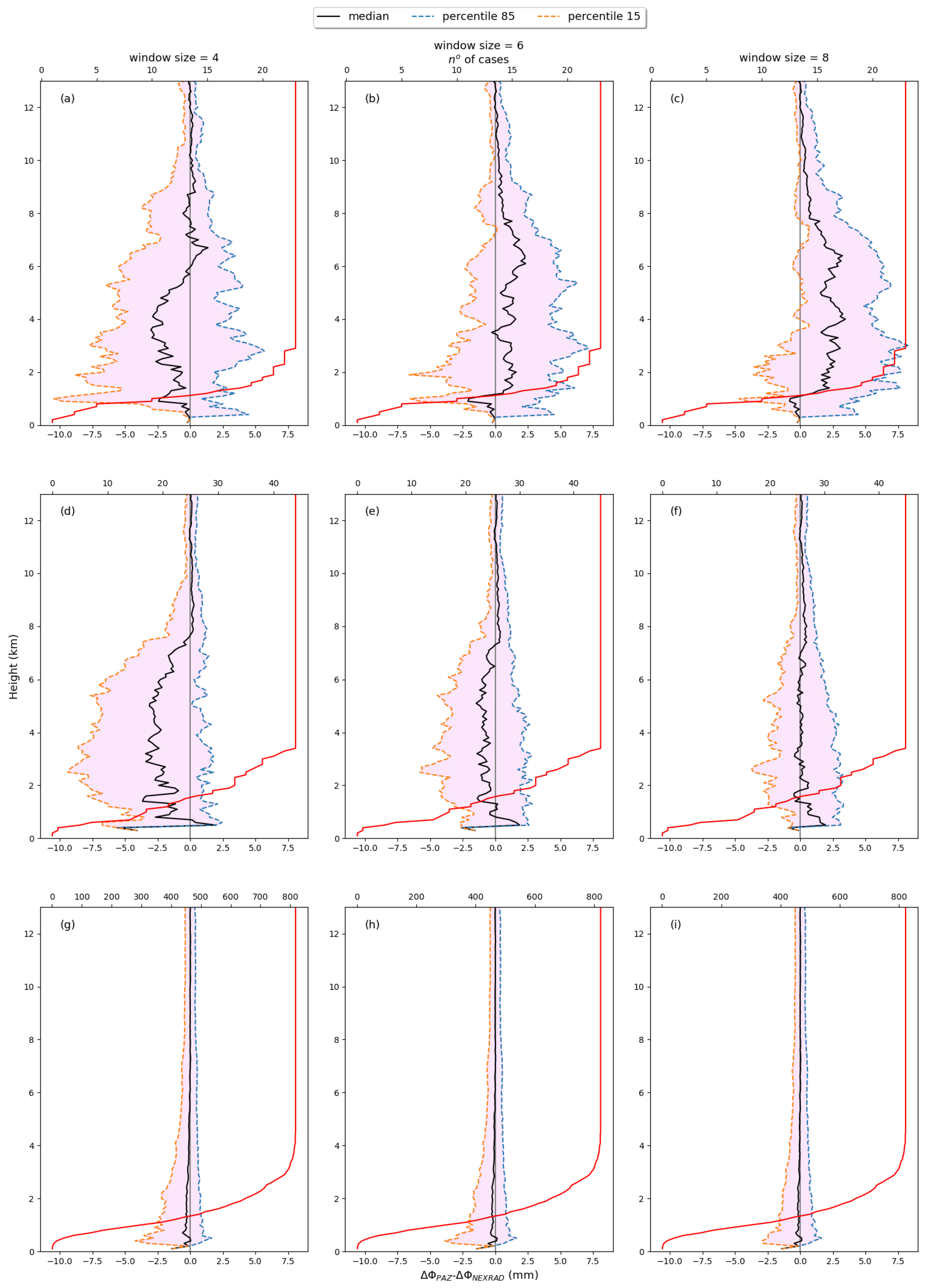
Figure 10.
Values of the echotop height obtained from NEXRAD and PAZ datasets for two different thresholds, dBZ and dBZ.
Figure 10.
Values of the echotop height obtained from NEXRAD and PAZ datasets for two different thresholds, dBZ and dBZ.

Table 1.
Number of cases employed in the analysis depending on the restrictions applied. The represents the mean between 0–10 km and cc is the correlation coefficient between the profiles. In some cases the number of observations will depend on the window size, such as , so for this tables the number of cases correspond to the window size of four gates.
| Number of Cases | |
|---|---|
| Total | 3208 |
| ≥ area covered | 1076 |
| ≥ 1 mm | 221 |
| ≥ 1.5 mm | 117 |
| ≥ area covered and ≥ 1.5 mm | 51 |
| cc ≥ 0.6 | 290 |
| cc ≥ 0.8 | 127 |
| ≤ 1 mm | 2987 |
| ≤ 1 mm | 2898 |
| ≤ 1 mm and ≤ 1 mm | 2818 |
Disclaimer/Publisher’s Note: The statements, opinions and data contained in all publications are solely those of the individual author(s) and contributor(s) and not of MDPI and/or the editor(s). MDPI and/or the editor(s) disclaim responsibility for any injury to people or property resulting from any ideas, methods, instructions or products referred to in the content. |
© 2024 by the authors. Licensee MDPI, Basel, Switzerland. This article is an open access article distributed under the terms and conditions of the Creative Commons Attribution (CC BY) license (https://creativecommons.org/licenses/by/4.0/).
Share and Cite
MDPI and ACS Style
Paz, A.; Padullés, R.; Cardellach, E. Evaluating the Polarimetric Radio Occultation Technique Using NEXRAD Weather Radars. Remote Sens. 2024, 16, 1118. https://doi.org/10.3390/rs16071118
AMA Style
Paz A, Padullés R, Cardellach E. Evaluating the Polarimetric Radio Occultation Technique Using NEXRAD Weather Radars. Remote Sensing. 2024; 16(7):1118. https://doi.org/10.3390/rs16071118
Chicago/Turabian StylePaz, Antía, Ramon Padullés, and Estel Cardellach. 2024. "Evaluating the Polarimetric Radio Occultation Technique Using NEXRAD Weather Radars" Remote Sensing 16, no. 7: 1118. https://doi.org/10.3390/rs16071118
Note that from the first issue of 2016, this journal uses article numbers instead of page numbers. See further details here.