


Anisotropic Green Tide Patch Information Extraction Based on Deformable Convolution

1
College of Computer Science and Engineering, Shandong University of Science and Technology, Qingdao 266590, China
2
College of Electronic and Information Engineering, Shandong University of Science and Technology, Qingdao 266590, China
*
Author to whom correspondence should be addressed.
Remote Sens. 2024, 16(7), 1162; https://doi.org/10.3390/rs16071162
Submission received: 31 January 2024
/
Revised: 5 March 2024
/
Accepted: 23 March 2024
/
Published: 27 March 2024
(This article belongs to the Special Issue Artificial Intelligence and Big Data for Oceanography)
Abstract
:Green tides are marine disasters caused by the explosive proliferation or high concentration of certain large algae in seawater, which causes discoloration of the water body. Accurate monitoring of its distribution area is highly important for early warning and the protection of marine ecology. However, existing deep learning methods have difficulty in effectively identifying green tides with anisotropic characteristics due to the complex and variable shapes of the patches and the wide range of scales. To address this issue, this paper presents an anisotropic green tide patch extraction network (AGE-Net) based on deformable convolution. The main structure of AGE-Net consists of stacked anisotropic feature extraction (AFEB) modules. Each AFEB module contains two branches for extracting green tide patches. The first branch consists of multiple connected dense blocks. The second branch introduces a deformable convolution module and a depth residual module based on a multiresolution feature extraction network for extracting anisotropic features of green tide patches. Finally, an irregular green tide patch feature enhancement module is used to fuse the high-level semantic features extracted from the two branches. To verify the effectiveness of the AGE-Net model, experiments were conducted on the MODIS Green Tide dataset. The results show that AGE-Net has better recognition performance, with F1-scores and IoUs reaching 0.8317 and 71.19% on multi-view test images, outperforming other comparison methods.
1. Introduction
Green tides are harmful ecological phenomena in which certain large green algae (e.g., seaweed) in seawater explosively proliferate or aggregate under certain environmental conditions, causing discoloration of the water body. Large aggregations of green algae can block sunlight, consume oxygen in the water and affect the growth of other marine organisms, leading to a range of ecological and environmental problems [1], which in turn threaten coastal tourism and aquaculture [2,3]. Obtaining a rapid and accurate understanding of the dynamics of green tide events is essential for the protection of marine ecosystems.
Satellite remote sensing technology has the advantages of a large scale and a synchronous observation ability, and it plays an important role in green tide monitoring tasks, providing a variety of data sources for researchers to utilize. For example, the HJ-1 satellite [4], a Chinese environmental monitoring satellite, is equipped with multiple sensors, including optical sensors and microwave sensors, which can be used for monitoring and evaluating green tide disasters. The HY-1C satellite [5] is equipped with multiple sensors that provide ocean environmental monitoring data, including ocean surface temperature and ocean pigment concentration data, for monitoring and analyzing green tide disasters. The GF-1 satellite [6] has high-resolution optical remote sensing capabilities, providing detailed surface images for spatial distribution analysis and monitoring of green tide disasters. MODIS [7] is a widely used sensor for Earth observation and is used to monitor the distribution and evolution of marine algal blooms. Synthetic aperture radar (SAR) [8] can observe under any weather conditions, and SAR data sources can provide backscatter characteristics of the sea surface, helping to monitor the spatial distribution and drift direction of green tide disasters. As an emerging technology in the field of remote sensing, the Cyclone Global Navigation Satellite System (CyGNSS) can avoid the signal attenuation caused by clouds and fog, which strongly supports the development of remote sensing applications, such as algal bloom detection [9]. These data sources have played an important role in monitoring the origin, spatial distribution, and drift direction of green tide disasters [10,11,12,13].
In particular, MODIS images have large bandwidths, stable data sources, rich spectral information, and free accessibility, so they can ensure data continuity and wide-scale macroscopic monitoring of green tides. Therefore, at this stage, using MODIS images for green tide monitoring is a good choice. Yellow Sea green tide patches continue to drift and grow under the influence of summer monsoons and surface currents, and they have different distribution patterns on the sea surface, ranging from scattered small patches to large-scale ribbon-like and block-like patches. The floating green algae within a strip are not evenly distributed and are sometimes intermittent. Due to the anisotropic distribution characteristics of green tide patches in remote sensing images [14], accurate identification of green tide patches is highly challenging.
The common green tide information extraction methods include index-based methods and traditional machine learning methods. Hu et al. proposed a floating algal index (FAI) using red, near-infrared, and short near-infrared bands [15]. Wang Ning et al. compared and analyzed five commonly used vegetation index algorithms on MODIS data, and the results of the study showed that the NDVI is still the strongest and most stable algorithm for detecting green tides [16]. However, thresholds applicable to different images are difficult to determine due to the strong influence of environmental factors, such as illumination [17]. Xie et al. proposed an object-oriented random forest classification framework for green tide monitoring along the Yellow Sea coast [18]. Geng et al. used importance scores to select features for GF-3 SAR images and used a random forest algorithm to extract green tide information [19]. Although index-based methods and traditional machine learning methods can achieve better results in extracting green tides, they still have the disadvantages of relying on predesigned guidelines, poor adaptability to different datasets, and underutilization of green tide patch features.
The development of deep learning is a gradual evolutionary process. The proposal of the back propagation algorithm [20] in 1960 solved the problem of training multilayer neural networks and laid the foundation for deep learning. Convolutional neural networks [21] have made significant breakthroughs in tasks such as image recognition, object detection, and image segmentation by efficiently extracting image features. In 2012, AlexNet’s victory in the ImageNet image classification challenge marked an important breakthrough in deep learning [22]. In 2014, the proposal of the generative adversarial network [23] pushed forward the development of generative modeling. In 2017, the Transformer [24] model abandoned the traditional loop and convolution structure and introduced the self-attention mechanism, which was able to compute and capture long-distance dependencies in sequences in parallel and has been widely used in various fields. The development of deep learning has not only increased the progress of computer vision, natural language processing and speech recognition but also brought new possibilities for practical applications.
As a biological phenomenon in water bodies, green tide outbreaks have a significant impact on the environment and ecosystem. There are many commonalities between remote-sensing water body extraction and green tide extraction in terms of the data sources, image processing methods and analysis methods used. In addition, in terms of water quality monitoring and environmental protection, accurate water body extraction is highly important for assessing the pollution status of water bodies and providing early warning of green tide outbreaks. In the field of remote sensing, the powerful feature learning and generalization capabilities of deep learning provide a new solution for the automatic extraction of water bodies [25,26] and green tides [27,28]. Previous studies have introduced convolutional neural network-based architectures for algae detection. For example, Gao et al. designed a deep learning framework, Algae-Net, based on U-Net, for detecting suspended green algae in MODIS images and SAR images [29]. Guo et al. constructed a deep learning automatic detection program for studying the distribution characteristics of green algae in the Yellow Sea off the coast of China [30]. Javier et al. proposed ERIS-Net, a macroalgae monitoring algorithm based on deep learning for detecting macroalgae in the Gulf of Mexico [31]. Cui et al. introduced the super-resolution technique and dense convolutional neural network into green tide monitoring for the first time, which improved green tide segmentation by reducing mixed pixels in MODIS remote sensing images [32].
However, the backbone networks used in the present work, such as Dense-Net and U-Net, use regular convolution, where the convolution kernel is usually fixed in shape and size; moreover, this convolution kernel is poorly adapted to targets with different scales or deformations and has poor generalizability. Dai et al. proposed deformable convolution [33], which adds an offset variable to each sampling point location in the convolution kernel, allowing for random sampling near the current location without limitation to the previous regular grid points and thus allowing for a closer approximation of the shape and size of the object during the sampling process. Due to the characteristic offset property, deformable convolution can better cope with targets with more complex deformations, such as green tide patches with more irregular shapes and scales.
Green tide patches have complex and variable shapes and a wide range of scales. To date, there is no information extraction model specifically designed for the characteristics of green tide patches with extremely irregular shapes and large-scale variations. Therefore, incomplete or missing information extraction for green tide patches is very common. To address this issue, we propose an anisotropic green tide patch information extraction method based on deformable convolution—AGE-Net. The IGPL (Irregular Green tide Patch feature Learning) module proposed in this paper can be better adapted to green tide patches with complex shapes and large-scale variations, thus solving the issue of variable size and shape of green tide patches. We analyzed the performance of AGE-Net on two test images through qualitative and quantitative comparisons with the results of other traditional extraction methods and deep learning extraction methods. Through experiments on the model structure, we determined the optimal depth of the model and conducted ablation experiments on the modules in AGE-Net to verify the effectiveness of each module in improving network performance.
2. Methods
2.1. AGE-Net
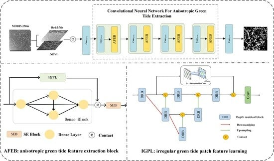
Detailed features are easily lost during green tide information extraction, and traditional convolution has difficulty determining the anisotropic distribution characteristics of green tide targets. Therefore, in this paper, a new full-resolution convolutional neural network model is proposed, the anisotropic green tide information extraction network (AGE-Net), which is based on deformable convolution; its overall architecture is shown in Figure 1.
The input for AGE-Net is a pseudo-color remote sensing image consisting of a red band, near-infrared bands, and calculated NDVIs, which can be represented by Equation (1):
where is the reflectance in the near-infrared band and is the reflectance in the red band. The output is a binary segmentation map, where 1 (white pixels) represents green tides and 0 (black pixels) represents seawater or other areas.
The main body of AGE-Net utilizes multiple information extraction stages. Each information extraction stage consists of 3 × 3 convolutional and anisotropic green tide feature extraction (AFEB) modules, which mainly obtain semantic information about green tides in the image; the richer the semantic information extracted by the AFEB is, the better the final green tide recognition effect. As shown in Figure 2, each AFEB contains two parallel branches, one of which is a dense block for extracting backbone information, and the other of which is an irregular green tide patch feature learning (IGPL) module, which is used to enhance the extraction of green tides at different scales and morphologies. Finally, the information extracted from the backbone network and the IGPL is fused by the SE block [34] to obtain a green tide feature map enhanced by channel selectivity.
2.2. Irregular Green Tide Patch Feature Learning Module
Considering the anisotropic characteristics of green tide patch targets, this paper proposes an IGPL module inspired by HRNet, as shown in Figure 3. The receptive field of ordinary convolutional filters cannot accurately match the shapes of green tide patches. To capture the characteristics of green tides more accurately, IGPL extracts green tide patch information through parallel information extraction branches. A branch is connected through down-sampling and a deep residual block (DRB), which not only increases the receptive field but also captures the multiscale contextual information of green tide patches, providing additional semantic information about green tide patches at different scales. The structure of the DRB is shown in the lower right corner of Figure 3. At the same time, another branch of the module performs deformable convolution operations on the input feature map to learn the complex morphological characteristics of green tides from the receptive field that is closest to the shape of the green tide. Finally, through the contact operation and 1 × 1 convolution, the anisotropic green tide patch features extracted by the deformable branch are integrated, and the multiscale green tide patch features extracted by the multiscale branch are extracted. Multiscale parallel green tide patch information extraction consists of three serial branches and three parallel branches. Assuming that the input is , the input of each DRB block can be expressed as shown in Equation (2).
where represents the input of the -th DRB in the i-th layer, represents the pooling operation, represents the upsampling operation, and represents the splicing operation.
2.3. Experimental Environment and Settings
We implemented the model using PyTorch 1.10.1. The operating system used was Ubuntu 18.04, and the graphics card was an NVIDIA GeForce RTX 2080Ti (NVIDIA Corporation, Santa Clara, CA, USA). The network training method used the SGDM optimizer, with 200 training epochs, an initial learning rate of 0.004, and a batch size setting of 8.
2.4. Evaluation
We use five evaluation metrics, namely, the accuracy, precision, recall, F1 score, and , to measure and evaluate the different green tide information extraction models. The definitions of the evaluation indicators are shown in Equations (3)–(7).
The value range of the above five evaluation indicators is 0–1, and the closer the value is to 1, the better the performance. The true positives () represent the number of pixels in the true value map where a green tide sample is detected as a green tide sample by the model. The true negatives () represent the number of pixels in the true value map, where a seawater sample is detected as seawater. The false positives () represent the number of pixels of seawater samples that the model predicts as green tide. The false negatives () are samples that are predicted by the model as seawater that are actually green tide samples.
3. Research Area and Data Pre-Processing
3.1. Study Area
The main research area of this paper is the Yellow Sea in eastern China. During the development process, the Yellow Sea green tide drifted and grew continuously, driven by the summer monsoon and surface currents in southern Jiangsu, gradually drifting northward toward the Yellow Sea, with both the affected area and coverage density continuously expanding. The Yellow Sea Enteromorpha prolifera population has been growing since 2008, and its annual green tide coverage and drift path have undergone significant changes but have not weakened. The maximum coverage area from 2009 to 2019 was more than 50,000 square kilometers. Most of the waters and coastlines in the Shandong Peninsula have been greatly affected, with a total affected coastline length of more than 1000 km, meaning that it is considered the largest green tide in the world.
The Yellow Sea has experienced a large-scale outbreak of green tides for 15 consecutive years, and this is a typical case of the frequent occurrence of green tides in the sea area. This paper selects the waters of the South Yellow Sea and its adjacent areas (33°–38°N, 119°–123°E) as the study area. The main study area is shown in Figure 4 and mainly includes the waters of Qingdao, Rizhao and Lianyungang.
3.2. Data Preprocessing
The MODIS remote sensing satellites make observations in 36 bands, of which the resolution of the first–second bands is 250 m, the resolution of the third–seventh bands is 500 m, and the resolution of the other bands is 1000 m. In our study, we use the raw data of 250 m resolution remote sensing images, which include both red and near-infrared bands.
In the data pre-processing stage, we pre-processed the selected multi-scene MODIS images with good imaging conditions and low cloud coverage by using Environment for Visualizing Images (ENVI) software (version 5.3) for geometric correction and cropping. After the preprocessing of the MODIS remote sensing images, the green tide boundary was manually drawn as the ground truth in ArcGIS through the manual visual interpretation method. We linearly transformed the original data using min–max normalization and cropped it to a 64 × 64 size. A dataset containing 920 images was obtained, and we divided the images into training and validation sets at a ratio of 9:1. In addition, an image outside the region of training data was selected and cropped to 5 images of size 256 × 256 as the experimental test set.
4. Results
4.1. Experiments
4.1.1. Comparative Experiment
We compared our proposed method with traditional methods for extracting green tides, including the normalized difference vegetation index (NDVI), ratio vegetation index (RVI), and support vector machine (SVM) [35]. Through multiple experiments on the test images, the optimal thresholds for NDVI and RVI were determined to be 0.05 and 1.10, respectively, with the optimal threshold obtained by the OTSU method. In addition, we compared the proposed method with current popular deep learning methods, including U-Net [36], ABC-Net [37], Algae-Net [29], and SRSe-Net [32]. For each model, we used the same training strategy to ensure fairness.
Table 1 shows the quantitative results of the different classification methods on the entire validation set. SVM is a pixel-level classifier and our training data is in the patch type. Therefore, while pre-processing the image data, we perform a flattening operation on each patch in the image and then stitch all the flattened patches together to form a whole. The labels are also processed in the same way. This converts the patch-type image and label data into a form that can be used to train the pixel-based SVM classifier. As the annotation of the green tide is performed by visual interpretation, the change of seawater color at the edge of the patch is not obvious, so it is inevitable that there will be a small number of incorrectly annotated samples. This could be the reason for the poor extraction of the SVM. Due to the sensitivity of green tides to NDVI values, the F1-score and IoU based on the NDVI threshold method reached 0.7812 and 64.10%, respectively. Compared to traditional machine learning methods, methods based on deep learning achieved better performance. SRSe-Net applies super-resolution technology to green tides, and it achieved F1-scores 0.0885 and 0.0261 higher than those of ABCNet and SRSe-Net, respectively. AGE-Net is significantly superior to the other comparison methods in terms of accuracy, F1 score, and IoU, with the F1 score and IoU reaching 0.8317 and 71.19%, respectively.
To further analyze the performance of the proposed model, we selected four test images from the test set. The visualization results and quantitative analysis are shown in Figure 5, Figure 6, Figure 7 and Figure 8. In Figure 5, image Figure 5a is the MODIS image used for testing, and image Figure 5b is the true value image, where the white area represents the green tide and the black area represents seawater. In the classification image, green represents correctly extracted green tide regions, red represents green tide regions predicted as seawater, white represents seawater regions predicted as green tide, and black represents correctly predicted seawater regions.
In Figure 6 and Figure 7, the test images have many small areas of green tide distribution, and the spectral-based NDVI, RVI, and SVM identify most of the small areas as seawater. Compared to traditional classification methods, methods based on deep learning consider the spatial information of green tides, reducing the misclassification of green tides in small areas. There are many misclassifications at the edge of the green tide distribution area when using U-Net and ABC-Net. Algae-Net, SRSe-Net and AGE-Net have better classification visualizations. Since AGE-Net considers the anisotropy of green tides, it extracts the green tide region more accurately than do the other models.
4.1.2. Interference Experiment
To verify the performance of the method in real applications and its robustness to complex scenes, we conducted interference experiments. Cloud cover and its impact on light changes may interfere with image recognition and extraction. Therefore, we chose images with partial cloud cover as test samples for our experiments. The visualization results and quantitative analysis are shown in Figure 9 and Table 2.
In Figure 9, the pink area in image Figure 9a is the cloud layer, and the red areas in images Figure 9c–j represent green tides that have not been extracted. The index-based (NDVI, RVI) methods with the optimal thresholds selected by the OTSU performed well in avoiding false extraction (99.97% and 99.95% precision for NDVI and RVI, respectively), but many green tide patches were not extracted, so the overall evaluation is not satisfactory. This indicates that, when dealing with complex scenes, there is some bias in the optimal threshold selected by OTSU. SVM outperforms threshold segmentation methods in distinguishing green tide patches from clouds. Deep learning methods are more effective at distinguishing green tide patches from clouds but tend to become confused at the boundary between them. In comparison, AGE-Net generates fewer false positives, and its classification results are closer to the ground truth. The F1-score and IoU of AGE-Net are 0.7963 and 66.16%, respectively, outperforming the other comparative methods. This shows that our method can maintain a high accuracy rate in the presence of cloud interference, which verifies the robustness of the method in complex environments.
4.1.3. Ablation Experiment
To verify the effectiveness of each module in AGE-Net, this section reports ablation experiments conducted on the network structure. AGE-Net uses only the dense structure as the baseline network. In the ablation experiment, four scenarios are considered: (1) a baseline network consisting of dense structures; (2) the network after adding the IGPL module; (3) the network after adding the SEB module; and (4) the network with both the IGPL and SEB modules, known as AGE-Net.
In Table 3, the bold values represent the best values of the methods in this evaluation index. As shown in Table 3, after adding the IGPL module to AGE-Net, the recall rate increased by 0.76%, and the F1-score increased by 0.0076. It has been proven that the introduction of deformable convolution can reduce the misidentification of seawater as green tides, enhance information extraction in low-coverage areas, and enhance the accuracy of recognition in boundary areas. After adding the SEB module, the accuracy rate increased by 4.26%, and the F1-score increased by 0.0105. It has been proven that multiscale feature fusion is very helpful in enhancing the extraction of green tide information, and the extraction of green tide patches at different scales can be enhanced through multiscale fusion. Compared to the baseline network, AGE-Net achieves optimal recall and F1-score performance with an increase of only 0.84 M in the number of parameters, achieving 87.28% and 0.8317, respectively. This approach greatly reduces the missed extraction of green tides and improves the extraction of difficult samples.
4.1.4. Model Performance Analysis and Parameterization Experiments
The proposed AGE-Net method uses deformable convolution to address the anisotropy problem of green tide patches. We compared the feature maps output by deformable convolution with those output by regular convolution to determine the effectiveness of the AGE-Net method in extracting green tide patches with anisotropic features.
According to the three examples in Figure 10, deformable convolution can more accurately capture the different morphologies and rich details of green tide patches, while standard convolution produces green tide patch feature maps that look blurry. Therefore, deformable convolution can be used to effectively learn the anisotropic features of green tide patches.
We evaluated the computational performance of the AGE-Net model. With an NVIDIA GeForce RTX 2080Ti GPU, the average inference time for processing a 256 × 256 test image was 423.69 ms, while the model training time for 200 epochs was 95 min.
To verify the effectiveness of the parameterization of the AGE-Net model proposed in this paper, experiments with different parameters were conducted. Sensitivity analysis experiments were performed on the entire test set for three parameters: the optimizer, batch size, and learning rate. The optimizers used were stochastic gradient descent (SGD), stochastic gradient descent with momentum (SGDM), and adaptive momentum estimation (ADAM). The batch sizes were set to 16, 8, 4, and 2. The learning rates were initialized to 0.0001, 0.001, and 0.004. When experimenting with one of the parameter settings, the other parameters remained unchanged. The results of the quantitative analysis of the sensitivity of the model parameters are shown in Table 4.
5. Discussion
Considering the anisotropic characteristics of green tide patches in remote sensing images, AGE-Net introduces deformable convolution for green tide information extraction, which has significant advantages in dealing with green tide patches with different morphologies and scales. Compared with previous methods, AGE-Net is able to accurately detect green tide patches and reduce the missed alarm rate; thus, it has good practicability.
Due to the limited spatial resolution of MODIS images, the geometric features of green tide patches extracted by AGE-Net are not sufficiently clear. In the future, we will introduce high-resolution images and super-resolution techniques to improve the ability in accurately identifying the boundaries of green tide patches while optimizing the estimation of patch area and even Enteromorpha prolifera biomass. In addition, the time cost of manually generating green tide training data is high, and we will explore low-cost annotation methods, such as scene-level annotation and scribble annotation, to improve the accessibility of deep learning methods for green tide extraction.
AGE-Net performs very well in the green tide extraction task and, theoretically, the method can also be applied to dynamic monitoring tasks for other marine ecological hazards with large variations in morphology and size, such as red tides, oil spills, ice melting, and marine debris.
6. Conclusions
This paper proposes a remote sensing monitoring model for green tides, AGE-Net. The main part of AGE-Net uses multiple information extraction stages to extract anisotropic features. The IGPL module utilizes parallel branches with multiple resolutions to obtain large-scale green tide information with low resolution and large receptive fields for information supplementation, and it enhances anisotropic feature extraction through deformable convolutional branches. The experimental results on the MODIS green tide dataset indicate that (1) AGE-Net has better classification performance in scattered, strip-shaped green tide distribution areas than do the other comparison methods, and (2) the combination of multiscale modules and deformable convolution effectively solves the problems of erroneous and missed extraction of green tides due to their anisotropic distribution characteristics.
Author Contributions
Conceptualization, B.C.; methodology, B.C. and M.L.; software, H.Z. and R.C.; validation, M.L., R.C. and X.Z.; investigation, B.C.; resources, X.Z.; writing—original draft preparation, M.L.; writing—review and editing, B.C. and M.L. All authors have read and agreed to the published version of the manuscript.
Funding
This research was funded by the National Natural Science Foundation of China, grant number 42276185, and the National Natural Science Foundation of Shandong Province, grant number ZR2020MD099.
Data Availability Statement
The data used in this study are available on GitHub. You can find them at the following link: https://github.com/chenruipeng123/AgeNet.
Acknowledgments
The authors would like to thank all the reviewers and editors for their comments on this paper.
Conflicts of Interest
The authors declare no conflicts of interest.
References
- Wang, M.; Zheng, W.; Li, F. Application of Himawari-8 Data to Enteromorpha Prolifera Dynamically Monitoring in the Yellow Sea. J. Appl. Meteor. Sci. 2017, 28, 714–723. [Google Scholar]
- Xing, Q.G.; An, D.Y.; Zheng, X.Y.; Wei, Z.N.; Wang, X.H.; Li, L.; Tian, L.Q.; Chen, J. Monitoring Seaweed Aquaculture in the Yellow Sea with Multiple Sensors for Managing the Disaster of Macroalgal Blooms. Remote Sens. Environ. 2019, 231, 111279. [Google Scholar] [CrossRef]
- Xiao, Y.F.; Zhang, J.; Cui, T.W.; Gong, J.L.; Liu, R.J.; Chen, X.Y.; Liang, X.J. Remote sensing estimation of the biomass of floating Ulva prolifera and analysis of the main factors driving the interannual variability of the biomass in the Yellow Sea. Mar. Pollut. Bull. 2019, 140, 330–340. [Google Scholar] [CrossRef] [PubMed]
- Sun, L.E.; Cui, T.W.; Cui, W.L. Analysis of Confusion Factors in Extracting Green Tide Remote Sensing Information from Multiple Source Satellites. Remote Sens. Inf. 2015, 30, 8–12. [Google Scholar]
- Jiang, X.W.; Lin, M.S.; Zhang, Y.G. Progress in China’s Ocean Satellite and Its Applications. JRS 2016, 20, 1185–1198. [Google Scholar]
- Wang, R.; Wang, C.Y.; Li, J.H. Analysis of the Monitoring Capability of Green Tide in the Yellow Sea Using Multi source and Multi resolution Remote Sensing Images. J. Qingdao Univ. Nat. Sci. Ed. 2018, 31, 95–101, 106. [Google Scholar]
- Song, D.B.; Gao, Z.Q.; Xu, F.X.; Ai, J.Q.; Ning, J.C.; Shang, W.T.; Jiang, X.P. Remote Sensing Analysis of the Evolution of Enteromorpha Prolifera in the South Yellow Sea in 2017 Based on GOCI. Oceanol. Limnol. Sin. 2018, 49, 1068–1074. [Google Scholar]
- Wan, J.H.; Su, J.; Sheng, H. Feasibility Study on Utilizing Geostationary Orbital Satellites for Operational Monitoring of Green Tide. Acta Laser Biol. Sin. 2018, 27, 155–160. [Google Scholar]
- Zhen, Y.Q.; Yan, Q.Y. Improving Spaceborne GNSS-R Algal Bloom Detection with Meteorological Data. Remote Sens. 2023, 15, 3122. [Google Scholar] [CrossRef]
- Gao, S.; Huang, J.; Bai, T. Analysis of the Drift Path of the Yellow Sea Green Tide in 2008 and 2009. Mar. Sci. 2014, 38, 86–90. [Google Scholar]
- Wu, L.J.; Cao, C.H.; Huang, J.; Cao, Y.J.; Gao, S. Preliminary Study on Numerical Simulation of Emergency Tracing of the Yellow Sea Green Tide. Mar. Sci. 2011, 35, 44–47. [Google Scholar]
- Wu, M.Q.; Guo, H.; Zhang, A.D. Study on Spatial-temporal Distribution Characteristics of Enteromorpha Prolifera in Shandong Peninsula Waters from 2008 to 2012. Spectrosc. Spectr. Anal. 2014, 34, 1312–1318. [Google Scholar]
- Song, X.L.; Huang, R.; Yuan, K.L. Characteristics of Green Tide Disasters in the Eastern Coast of Shandong Peninsula. Mar. Environ. Sci. 2015, 34, 391–395. [Google Scholar]
- Yue, Z.Y. Research on Remote Sensing Image Segmentation Algorithm Based on Deep Convolutional Networks. Eng. Technol. Part II 2022. [Google Scholar] [CrossRef]
- Hu, C. A novel ocean color index to detect floating algae in the global oceans. Remote Sens. Environ. 2009, 113, 2118–2129. [Google Scholar] [CrossRef]
- Wang, N.; Huang, J.; Cui, T.W.; Xiao, Y.F.; Cai, X.Q. Capability Comparison of 5 Vegetation Indices for Detecting the Green Tide in Different Development Phases and the Application. Acta Laser Biol. Sin. 2014, 23, 590–595. [Google Scholar]
- Garcia, R.A.; Fearns, P.; Keesing, J.K.; Liu, D.Y. Quantification of Floating Macroalgae Blooms using the Scaled Algae Index. J. Geophys. Res.-Ocean 2013, 118, 26–42. [Google Scholar] [CrossRef]
- Xie, C.; Dong, J.Y.; Sun, F.F.; Bing, L. Object-oriented random forest classification for Enteromorpha prolifera detection with SAR images. In Proceedings of the 2016 International Conference on Virtual Reality and Visualization (ICVRV), Hangzhou, China, 24–26 September 2016; IEEE: Piscataway, NJ, USA, 2016; pp. 119–125. [Google Scholar]
- Geng, X.M.; Li, P.X.; Yang, J.; Shi, L.; Li, X.M.; Zhao, J.Q. Ulva prolifera detection with dual-polarization GF-3 SAR data. IOP Conf. Ser. Earth Environ. Sci. 2020, 502, 012026. [Google Scholar] [CrossRef]
- Werbos, P.J. Beyond Regression: New Tools for Prediction and Analysis in the Behavioral Sciences. Ph.D. Thesis, Harvard University, Cambridge, MA, USA, 1974. [Google Scholar]
- Lecun, Y.; Bottou, L.; Bengio, Y. Intelligent Signal Processing; IEEE Press: Piscataway, NJ, USA, 2001; pp. 306–351. [Google Scholar]
- Krizhevsky, A.; Sutskever, I.; Hinton, G.E. ImageNet classification with deep convolutional neural networks. Adv. Neural Inf. Process. Syst. 2012, 25, 1097–1105. [Google Scholar] [CrossRef]
- Goodfellow, I.; Pouget-Abadie, J.; Mirza, M.; Xu, B.; Warde-Farley, D.; Ozair, S.; Courville, A.; Bengio, Y. Generative Adversarial Nets. Adv. Neural Inf. Process. Syst. 2014, 27, 139–144. [Google Scholar]
- Ashish, V.; Noam, S.; Niki, P.; Jakob, U.; Llion, J.; Aidan, N.G.; Lukasz, K.; Illia, P. Attention Is All You Need. In Proceedings of the Conference on Neural Information Processing Systems, Long Beach, CA, USA, 4–9 December 2017; Volume 30, pp. 5998–6008. [Google Scholar]
- Miao, Z.M.; Fu, K.; Sun, H.; Sun, X.; Yan, M.L. Automatic Water-Body Segmentation From High-Resolution Satellite Images via Deep Networks. IEEE Geosci. Remote Sens. Lett. 2018, 15, 602–606. [Google Scholar] [CrossRef]
- Yan, Q.Y.; Chen, Y.H.; Jin, S.G.; Liu, S.C.; Jia, Y.; Zhen, Y.Q.; Chen, T.X.; Huang, W.M. Inland Water Mapping Based on GA-LinkNet From CyGNSS Data. IEEE Geosci. Remote Sens. Lett. 2023, 20, 1–5. [Google Scholar] [CrossRef]
- Cui, B.G.; Li, X.H.; Wu, J.; Ren, G.B.; Lu, Y. Tiny-Scene Embedding Network for Coastal Wetland Mapping Using Zhuhai-1 Hyperspectral Images. IEEE Geosci. Remote Sens. Lett. 2022, 19, 1–5. [Google Scholar] [CrossRef]
- Qin, Y.Q.; Chi, M.M. RSImageNet: A Universal Deep Semantic Segmentation Lifecycle for Remote Sensing Images. IEEE Access 2020, 8, 68254–68267. [Google Scholar] [CrossRef]
- Gao, L.; Li, X.F.; Kong, F.Z.; Yu, R.; Guo, Y.; Ren, Y. AlgaeNet: A Deep Learning Framework to Detect Floating Green Algae from Optical and SAR Imagery. IEEE J. Sel. Top. Appl. Earth Obs. Remote Sens. 2022, 15, 2782–2796. [Google Scholar] [CrossRef]
- Guo, Y.; Gao, L.; Li, X.F. Distribution Characteristics of Green Algae in Yellow Sea Using a Deep Learning Automatic Detection Procedure. In Proceedings of the 2021 IEEE International Geoscience and Remote Sensing Symposium IGARSS, Brussels, Belgium, 11–16 July 2021; pp. 3499–3501. [Google Scholar]
- Arellano-Verdejo, J.; Lazcano-Hernandez, H.E.; Cabanillas-Terán, N. ERISNet: Deep neural Network for Sargassum Detection along the Coastline of the Mexican Caribbean. PeerJ 2019, 7, e6842. [Google Scholar] [CrossRef] [PubMed]
- Cui, B.G.; Zhang, H.Q.; Jing, W.; Liu, H.; Cui, J. SRSe-Net: Super-resolution-based Semantic Segmentation Network for Green Tide Extraction. Remote Sens. 2022, 14, 710. [Google Scholar] [CrossRef]
- Dai, J.; Qi, H.; Xiong, Y.; Li, Y.; Zhang, G.; Wei, Y. Deformable Convolutional Networks. In Proceedings of the IEEE International Conference on Computer Vision, Venice, Italy, 22–29 October 2017; pp. 764–773. [Google Scholar]
- Hu, J.; Shen, L.; Sun, G. Squeeze-and-Excitation Networks. In Proceedings of the IEEE Conference on Computer Vision and Pattern Recognition, Salt Lake City, UT, USA, 18–23 June 2018; pp. 7132–7141. [Google Scholar]
- Cortes, C.; Vapnik, V. Support-vector networks. Mach. Learn. 1995, 20, 273–297. [Google Scholar] [CrossRef]
- Ronneberger, O.; Fischer, P.; Brox, T. UNet: Convolutional networks for biomedical image segmentation. In Proceedings of the Medical Image Computing and Computer-Assisted Intervention–MICCAI 2015: 18th International Conference, Munich, Germany, 5–9 October 2015; Springer International Publishing: Cham, Switzerland, 2015; pp. 234–241. [Google Scholar]
- Li, R.; Zheng, S.Y.; Zhang, C.; Duan, C.X.; Wang, L.B.; Atkinson, P.M. ABCNet: Attentive bilateral contextual network for efficient semantic segmentation of Fine-Resolution remotely sensed imagery. ISPRS J. Photogramm. Remote Sens. 2021, 181, 84–98. [Google Scholar] [CrossRef]
Figure 1.
The overall architecture of AGE-Net.

Figure 2.
A schematic diagram of the anisotropic green tide feature extraction block (AFEB).

Figure 3.
Schematic diagram of the irregular green tide patch feature learning (IGPL) module.

Figure 4.
Study area.

Figure 5.
Qualitative results for test image 1.

Figure 6.
Qualitative results for test image 2.

Figure 7.
Qualitative results for test image 3.

Figure 8.
Qualitative results for test image 4.

Figure 9.
Qualitative results for the test image.

Figure 10.
Visualization of feature maps. (The top row shows the feature maps generated by standard convolution, and the bottom row shows the feature maps generated by deformable convolution. A change from yellow to blue indicates that the activation value increases from low to high).
Figure 10.
Visualization of feature maps. (The top row shows the feature maps generated by standard convolution, and the bottom row shows the feature maps generated by deformable convolution. A change from yellow to blue indicates that the activation value increases from low to high).


Table 1.
Quantitative results of different methods.
| Method | Accuracy (%) | Precision (%) | Recall (%) | F1-Score | IoU (%) |
|---|---|---|---|---|---|
| NDVI (0.05) | 91.38 | 86.45 | 75.21 | 0.8043 | 64.10 |
| RVI (1.10) | 90.79 | 89.95 | 69.26 | 0.7826 | 62.65 |
| SVM | 91.50 | 89.41 | 55.96 | 0.6884 | 52.48 |
| U-Net | 92.30 | 89.11 | 61.65 | 0.7288 | 57.33 |
| ABC-Net | 91.83 | 83.17 | 64.31 | 0.7253 | 56.90 |
| Algae-Net | 93.09 | 81.31 | 76.38 | 0.7877 | 64.97 |
| SRSe-Net | 93.86 | 82.84 | 79.98 | 0.8138 | 68.61 |
| AGE-Net | 94.07 | 79.43 | 87.28 | 0.8317 | 71.19 |
The best result for each benchmark is in bold.
Table 2.
Quantitative results for the test image.
| Method | Accuracy (%) | Precision (%) | Recall (%) | F1-Score | IoU(%) |
|---|---|---|---|---|---|
| NDVI (0.30) | 78.90 | 99.97 | 23.93 | 0.3862 | 23.93 |
| RVI (0.19) | 76.01 | 99.95 | 13.49 | 0.2378 | 13.49 |
| SVM | 85.67 | 88.31 | 55.73 | 0.6833 | 51.90 |
| U-Net | 87.06 | 82.46 | 74.39 | 0.7058 | 59.23 |
| ABC-Net | 82.99 | 78.21 | 53.62 | 0.6362 | 46.65 |
| Algae-Net | 86.68 | 75.63 | 76.69 | 0.7615 | 61.49 |
| SRSe-Net | 87.93 | 80.54 | 74.46 | 0.7738 | 63.11 |
| AGE-Net | 88.59 | 78.86 | 80.42 | 0.7963 | 66.16 |
The best result for each benchmark is in bold.
Table 3.
Ablation experiment results.
| Method | Accuracy (%) | Precision (%) | Recall (%) | F1-Score | Parameters (M) |
|---|---|---|---|---|---|
| Baseline | 93.37 | 77.80 | 84.62 | 0.8107 | 6.62 |
| Baseline + IGPL | 93.64 | 78.57 | 85.38 | 0.8183 | 7.39 |
| Baseline + SEB | 93.99 | 82.06 | 82.19 | 0.8212 | 7.17 |
| AGE-Net | 94.07 | 79.43 | 87.28 | 0.8317 | 7.46 |
The best result for each benchmark is in bold.
Table 4.
Model parameter sensitivity experiment.
| Parameter Name | Parameter Value | F1-Score | IoU |
|---|---|---|---|
| Optimizer | SGD | 0.8243 | 0.7091 |
| SGDM | 0.8317 | 0.7119 | |
| ADAM | 0.8311 | 0.7110 | |
| Batch size | 16 | 0.8298 | 0.7012 |
| 8 | 0.8315 | 0.7119 | |
| 4 | 0.8292 | 0.7082 | |
| 2 | 0.8216 | 0.6972 | |
| Learning rate | 0.004 | 0.8317 | 0.7119 |
| 0.001 | 0.8257 | 0.7031 | |
| 0.0001 | 0.8132 | 0.6851 |
The best result for each benchmark is in bold.
Disclaimer/Publisher’s Note: The statements, opinions and data contained in all publications are solely those of the individual author(s) and contributor(s) and not of MDPI and/or the editor(s). MDPI and/or the editor(s) disclaim responsibility for any injury to people or property resulting from any ideas, methods, instructions or products referred to in the content. |
© 2024 by the authors. Licensee MDPI, Basel, Switzerland. This article is an open access article distributed under the terms and conditions of the Creative Commons Attribution (CC BY) license (https://creativecommons.org/licenses/by/4.0/).
Share and Cite
MDPI and ACS Style
Cui, B.; Liu, M.; Chen, R.; Zhang, H.; Zhang, X. Anisotropic Green Tide Patch Information Extraction Based on Deformable Convolution. Remote Sens. 2024, 16, 1162. https://doi.org/10.3390/rs16071162
AMA Style
Cui B, Liu M, Chen R, Zhang H, Zhang X. Anisotropic Green Tide Patch Information Extraction Based on Deformable Convolution. Remote Sensing. 2024; 16(7):1162. https://doi.org/10.3390/rs16071162
Chicago/Turabian StyleCui, Binge, Mengting Liu, Ruipeng Chen, Haoqing Zhang, and Xiaojun Zhang. 2024. "Anisotropic Green Tide Patch Information Extraction Based on Deformable Convolution" Remote Sensing 16, no. 7: 1162. https://doi.org/10.3390/rs16071162
Note that from the first issue of 2016, this journal uses article numbers instead of page numbers. See further details here.