
Methane Retrieval from Hyperspectral Infrared Atmospheric Sounder on FY3D
by
 , , ,
, , ,
Xinxin Zhang
1,2 ,
,
Ying Zhang
2,*, 
Fan Meng
2,
Jinhua Tao
2,
Hongmei Wang
1,
Yapeng Wang
3 and
Liangfu Chen
2 1
School of Electrical Engineering and Automation, Nantong University, Nantong 226019, China
2
Key Laboratory of Remote Sensing and Digital Earth, Aerospace Information Research Institute, Chinese Academy of Sciences, Beijing 100101, China
3
Key Laboratory of Radiometric Calibration and Validation for Environmental Satellites, National Satellite Meteorological Center, China Meteorological Administration, Beijing 100081, China
*
Author to whom correspondence should be addressed.
Remote Sens. 2024, 16(8), 1414; https://doi.org/10.3390/rs16081414
Submission received: 29 February 2024
/
Revised: 11 April 2024
/
Accepted: 12 April 2024
/
Published: 16 April 2024
(This article belongs to the Section Atmospheric Remote Sensing)
Abstract
:This study utilized an infrared spotlight Hyperspectral infrared Atmospheric Sounder (HIRAS) and the Medium Resolution Spectral Imager (MERSI) mounted on FY3D cloud products from the National Satellite Meteorological Center of China to obtain methane profile information. Methane inversion channels near 7.7 μm were selected based on the different distribution of methane weighting functions across different seasons and latitudes, and the selected retrieval channels had a great sensitivity to methane but not to other parameters. The optimization method was employed to retrieve methane profiles using these channels. The ozone profiles, temperature, and water vapor of the European Centre for Medium-Range Weather Forecasts (ECMWF) fifth-generation reanalysis data (ERA5) were applied to the retrieval process. After validating the methane profile concentrations retrieved by HIRAS, the following conclusions were drawn: (1) compared with Civil Aircraft for the Regular Investigation of the Atmosphere Based on an Instrument Container (CARIBIC) flight data, the average correlation coefficient, relative difference, and root mean square error were 0.73, 0.0491, and 18.9 ppbv, respectively, with lower relative differences and root mean square errors in low-latitude regions than in mid-latitude regions. (2) The methane profiles retrieved from May 2019 to September 2021 showed an average error within 60 ppbv compared with the Fourier transform infrared spectrometer (FTIR) station observations of the Infrared Working Group (IRWG) of the Network for the Detection of Atmospheric Composition Change (NDACC). The errors between the a priori and retrieved values, as well as between the retrieved and smoothed values, were larger by around 400–500 hPa. Apart from Toronto and Alzomoni, which had larger peak values in autumn and spring respectively, the mean column averaging kernels typically has a larger peak in summer.
1. Introduction
As one of the most abundant greenhouse gases in the atmosphere, the emissions of methane (CH4) account for about one-fifth of global emissions [1]. Methane’s heat-trapping capability is more than 25 times greater than that of carbon dioxide in the atmosphere and contributes 4–9% to the greenhouse effect (9–26% for carbon dioxide (CO2)). The global average mole fraction of CH4 in 2022 was 1923 ± 2 ppb, an increase of 16 ppb over the previous year (1908 ± 2) and 264% of the pre-industrial level of 722 ppb [2]. Although the increase in CH4 from 2021 to 2022 (16 ppb) was slightly lower than the increase from 2020 to 2021 (18 ppb), it still marked a significant increase from the annual growth rate over past years. In addition, CH4 is one of the most long-lived atmospheric gases, and makes up approximately sixteen percent of the total radiative forcing. Less than one-half of CH4 in the atmosphere comes from natural emissions [3], while the remaining is caused by emissions from human sources (such as ruminant animals, fossil fuel extraction, landfill sites, and biomass burning) [4,5]. The significant increase in greenhouse gases caused by human activities is the main factor contributing to global warming, which has become one of the most critical and far-reaching global environmental issues. Countries need to enact related policies based on scientifically reliable information in order to reduce greenhouse gas emissions and avoid the negative consequences of climate change. In this context, there is an increasing demand for existing and reliable greenhouse gas data to meet the needs of scientific research and provide information for decision-makers.
At present, the observation methods used to monitor atmospheric CH4 vertical profile mainly include in situ sampling and ground and satellite remote sensing technology. The Infrared Working Group (IRWG) of the Network for the Detection of Atmospheric Composition Change (NDACC) manages twenty solar viewing Fourier transform infrared spectrometers (FTIR) [6]. The ground-based FTIR stations can provide vertical profile data for CH4 [7], carbon monoxide (CO) [8], nitrous oxide (N2O) [9], ozone (O3) [10], and other atmospheric constituents for all continents. Aircraft/balloons and other platforms are mostly used for fixed-point directional experimental observation in order to obtain atmospheric CH4 vertical information. Civil Aircraft for the Regular Investigation of the Atmosphere Based on an Instrument Container (CARIBIC) has been studying important chemical and physical characteristics of CH4, CO, N2O, CO2 and aerosol in the upper troposphere and lower stratosphere of the Earth’s atmosphere [11]. Since the CARIBIC program was implemented in 2005, the program has typically measured flights once a month for two to four consecutive days with a time resolution of 1 s and calibrated every 25 min. CARIBIC flew mostly in the northern hemisphere, with only a small number of flights exploring the southern hemisphere. The advantages of traditional ground monitoring are its high reliability, its ease of use and its instantaneous results. However, the disadvantages are the way in which it is limited in the number and distribution of stations and its large consumption of manpower and material resources. In addition, due to the climate environment and the aging of instruments and equipment, long-term continuous observation data are often not available. Most sites are concentrated in the mainland, and marine data are scarce, which makes it impossible to accurately assess the exchange characteristics of CH4 concentration in the atmosphere, sea, and land under the dynamic cycle of the natural ecosystem. Airborne platforms are expensive and can only obtain vertical CH4 concentration information.
Compared with ground monitoring, satellite remote sensing provides a means to detect greenhouse gases in the global atmosphere. Especially with the rise of satellite detection technology in the past three decades, high space coverage and high-precision greenhouse gas detection is conducive to the study of global greenhouse effects. The thermal infrared (TIR) observations capable of observing CH4 include the infrared atmospheric sounding interferometer (IASI) on the METOP satellite [12], the atmospheric infrared sounder (AIRS) [13] on AQUA, the spectral infrared detector cross-track infrared sounder (CrIS) [14] carried by the national polar-orbiting environmental satellite system, Suomi-NPP and NOAA-20 of the US Earth observation satellite, and the infrared spotlight hyperspectral infrared atmospheric sounder (HIRAS) carried by the FY3D/FY3E launched by the National Satellite Meteorological Center of China [15]. The near-infrared (NIR) satellite sensors capable of observing CH4 include the atmospheric absorption spectral scanning imager (SCIAMACHY) on the European Space Agency’s ENVISAT satellite [16]; TanSat [17], a carbon satellite developed by China; the greenhouse gases observing satellite (GOSAT) launched by Japan [18]; the orbiting carbon observatory-2 (OCO-2) satellite [19] developed by the National Aeronautics and Space Administration (NASA); and the tropospheric monitoring instrument (TROPOMI) launched on the Sentinel-5 precursor (S5P) satellite [20]. Near-infrared satellite sensors primarily utilize the 1.647 μm absorption band to detect the column-averaged dry-air mole fractions of CH4 (XCH4). Nevertheless, this band depends on sunlight reflection and only performs well under clear-sky daytime and land conditions. Additionally, the accuracy of near-infrared CH4 retrieval is strongly dependent on aerosols, as it affects the near-infrared photon path in the atmosphere, which is a challenging task to estimate [21]. Thermal infrared satellite sensors mainly depend on the 7.7 μm absorption band to obtain CH4 profile information [22]. Xiong et al. presented the characteristics and verification of inverted CH4 profiles of AIRS. AIRS channels near 7.6 μm were applied to CH4 retrieval, and these channels showed the higher sensitivity to the upper and middle layers of the troposphere (approximately 250 hPa in tropical regions and 450 hPa in polar regions) [23]. Crevoisier et al. [24] employed a neural network approach with a multilayer perceptron to retrieve the global distribution of methane under clear-sky conditions for a period of 16 months. This incorporated IASI channels that partially covered the methane ν3 absorption band into the methane profile retrieval, which improved the accuracy of methane retrieval near the surface and increased the degrees of freedom in CH4 retrieval. Nalli et al. have provided an overview of the verification of the atmospheric greenhouse gases profile which was obtained from CrIS. CH4 product accuracies were within ±1%, with precisions of ≈1.5% [25]. The band settings of HIRAS are similar to CrIS, which can also detect temperature, humidity, and greenhouse gases. Li et.al. [26] utilized the data of HIRAS sensors on FY-3E to obtain atmospheric profiles of O3, CO, and CH4 using the convolutional neural network model (CNN) and the U-shaped network model (UNET). When comparing Medium-Range Weather Forecasts Atmospheric Composition Reanalysis v4 (EAC4) data with the CH4 profiles retrieval results, the research findings indicate that the mean percentage error across all layers for data from CNN and UNET was below 0.7% [26]. At present, the research on CH4 gas retrieval based on thermal infrared satellite sensors such as AIRS, IASI and CrIS has been very mature, and there are even official satellite products. However, the research on atmospheric CH4 profiles based on HIRAS is still lacking, especially in the case of FY3D-HIRAS, and there is no official CH4 profile product available. In this paper, we performed CH4 retrieval based on FY3D-HIRAS.
The methane profile retrieval algorithms for TIR sensors can be broadly categorized into two types. The first type comprises statistical methods, such as regression statistical methods based on empirical orthogonal functions [22] and neural network algorithms [27]. Statistical methods, which do not directly solve equations, have certain advantages in terms of computational efficiency and solution stability. However, these methods rely heavily on the profiles of training samples and may not capture the physical significance of radiative transfer, making them unsuitable for data-scarce regions. The second type comprises physical inversion algorithms, which involve optimization algorithms that consider the forward atmospheric model. The theoretical framework of physical inversion algorithms was proposed by Rodgers [28]. This method utilizes the prior information to constrain the model solution and simulates the atmospheric parameters based on the forward radiative transfer model. It approximates the true solution using methods like Newton iteration. Currently, optimization estimation methods are widely used for atmospheric CH4 retrieval. Through the comparison between AIRS retrieved CH4 profiles based on physical retrieval methods [29] and aircraft CH4 profiles, Xiong et al. [23] concluded that the accuracy was 0.5–1.6%. Moreover, the information content in the tropics was greater than that in high latitudes. Nicholas et al. analyzed the global performance of the NUCAPS carbon gas profile EDR, and found that the CrIS CH4 profiles product had an accuracy of ±1% and a precisions of ≈1.5% throughout the tropospheric column [25]. Xiong et al. adopted the physical retrieval algorithm to retrieve IASI CH4 vertical profiles. Their findings reveal that the degrees of freedom were mostly below 1.5, with the maximum sensitivity occurring in the pressure of 100–600 hPa and 200–750 hPa in the tropics and in the mid-to-high latitudes, respectively [30]. Li et al. [26] applied CNN to obtain CH4 and other atmospheric profile components based on the HIRAS that is on board the Fengyun-3E. For CH4 profile retrieval, mean percentage error, and root-mean-square error of the whole layer, the results in relation to Medium-Range Weather Forecasts Atmospheric Composition Reanalysis v4 (EAC4) data were less than 0.7% and 1.5 × 10⁻⁸ kg/kg, respectively. Currently, CH4 inversion studies based on TIR sensors such as AIRS, IASI and CrIS have reached a mature stage, with official satellite products available. However, research on atmospheric CH4 profiles using FY3D-HIRAS is still lacking. In this paper, we realize CH4 profile retrieval based on the TIR sensor HIRAS aboard the FY3D, the retrieval method, its validation, and the uncertainty analysis. The article contains the following sections: Section 2 introduces the HIRAS and MERSI detectors, as well as the validation data used in Section 4. Section 3 explains key steps of the methane profile inversion algorithm. The retrieval results and verification are detailed in Section 4. Finally, Section 5 and Section 6 respectively give the final discussion and conclusion.
2. Data
2.1. HIRAS and MERSI
The Fengyun-3 D satellite (FY3D) was launched in November 2017. The infrared hyperspectral atmospheric sounding instrument (HIRAS) is the first interferometric infrared hyperspectral sounding equipment on a polar-orbiting satellite platform in China. It has 2275 channels with a spectral resolution of 0.625 cm−1 in the spectral range of 3.92 μm to 15.38 μm. During earth observation, the scanning mirror performs cross-orbit transverse scanning, and a total of 29 resident fields of view are observed. Each field of view includes 4 pixels (2 × 2 probe array), and the spatial resolution of nadir points is 16 km. The infrared band was divided into long, medium, and short wave bands, among which the long wave infrared had 777 channels and a spectral range of 650~1135 cm−1 (15.38~8.8 μm). There are 865 mid-wave infrared channels, and their spectral range is 1210~1750 cm−1 (8.26~5.7 μm). There are 633 short-wave infrared channels, and their spectral range is 2155~2550 cm−1 (4.64~3.92 μm). This paper utilized the national satellite meteorological center which provided FY3D HIRAS level 1 Data (http://satellite.nsmc.org.cn/portalsite/default.aspx, accessed on 15 June 2023). HIRAS L1 data are generated after multi-step preprocessing and spectral radiometric calibration. This can be directly applied in satellite data assimilation; in climate model study, which is also widely used in the atmospheric vertical profiling; and in the detection of cloud, atmospheric components, and outgoing longwave radiation.
The medium resolution spectral imager type II (MERSI-II) mounted on FY3D integrates the functions of the original two imaging instruments (MERSI and a visible infrared scanning radiometer (VIRR)) of the Fengyun-3 satellite, and the spectral channels have been expanded from the original 20 channels to 25 channels [31]. Among these, there are 6 visible bands, 10 visible infrared bands, 3 short-wave infrared bands and 6 medium-to-long-wave infrared bands, the spectral coverage range is 470~12,000 nm, and the spatial resolution is 250 m to 1 km [32]. This is the first imaging instrument in the world that can obtain data regarding the global 250 m resolution infrared split window region. It can obtain global true color images, with 250 m resolution every day without gaps, and the retrieval results for atmospheric, terrestrial and oceanic parameters, such as clouds, aerosols [31], water vapor, surface characteristics [33] and ocean water color, achieved a high accuracy. It provides scientific support for China’s ecological management and restoration, environmental monitoring, and protection. It also provides China’s observation program for global ecological environment, disaster monitoring and climate assessment. This study obtained FY3D/MERSI-II cloud data (the global cloud cover (CLA) product data) of the satellite remote sensing data from the National Satellite Meteorological Center service network (http://satellite.nsmc.org.cn/portalsite/default.aspx, accessed on 15 June 2023). The CLA products include global daily total cloud cover and high-level cloud cover. Total cloud cover refers to the radiation ratio between all cloud pixels and clear pixels within a given area, with valid values ranging from 0% to 100%, where 0% represents clear sky and 100% represents cloudy sky. These products are projected onto a global latitude–longitude grid of 180° × 360° with a resolution of 0.05°. In the article, we consider pixels with a total cloud cover of less than 30% to be “clear sky”, in order to ensure a sufficient amount of data for analysis and to maintain the accuracy of the retrieval.
2.2. ERA5
Reanalysis v5 (ERA5) [34] is a reanalysis dataset from the European Union. The data are developed by the Copernicus Climate Change Service (C3S), and operated by the European Centre for Medium-Range Weather Forecasts (ECMWF). ERA5 reanalysis data have improved upon that of its predecessor, ERA-Interim. After the upgrade, the spatial and temporal resolution of the data have been greatly improved. Users can obtain the atmospheric composition information from the official website with a horizontal resolution of 31 km and about 80 km from the surface to the ground above (pressure 0.01 hPa). The temporal resolution of the data is one hour. The atmospheric composition is divided into 137 layers. In contrast with the ERA5, its predecessor only has an 80 km spatial resolution and the temporal resolution is not hourly, providing data every six hours that is divided vertically from the surface up to 60 layers. In addition, for the first time, the ERA5 reanalysis data consist of a 10-member ensemble reanalysis product. The spatial resolution of ERA5 increased to 62 km, and the temporal resolution of 1 h could be used to assess atmospheric uncertainties. The unique advantage of the above ERA5 data is that they are based on the data assimilation ensemble system developed by the ECMWF, which can detect differences in actual observations and forecasts and provide users with more information about atmospheric parameters at different times and places. By introducing a large amount of historical data and satellite monitoring data into the data assimilation and model system, the ERA5 dataset can provide users with relatively accurate real-time atmospheric information. The acquisition and use of the above data and other relevant information will also be disclosed to users. ERA5 provides 140 more variables than its predecessor, including wave height, wave direction, etc., enabling users to analyze atmospheric and oceanic historical information more conveniently and accurately. Temperature, humidity, and ozone profile data used as inputs in radiative transfer for TOVS (RTTOV) [35] are from ERA5.
2.3. Validation Data
CARIBIC (http://www.caribic-atmospheric.com/, accessed on 28 November 2022) researches and monitors important chemical and physical processes of trace gases and aerosol particles in the upper troposphere and lower stratosphere [11]. Since the CARIBIC program was implemented in 2005, it has typically measured flights once a month for two to four consecutive days with a time resolution of 1 s and a calibration every 25 min. CARIBIC planes flew mostly in the northern hemisphere, with only a small number of flights in the southern hemisphere. In this paper, after May 2019, data from only four flights were available for comparison and validation, and the obtained CARIBIC data were synthesized into time intervals of 10 s and 2 min. The four flights were collected at various locations within a narrow range of altitudes. These flights cover a wide area, and most measurements were made at cruising altitudes of around 9–12 km, such as mid-tropical tropospheric air or mid-high latitude upper tropospheric air and lower tropospheric air. Gas sampling is generally executed at cruising altitude, and most of the CH4 data selected in this part are concentrated in the range of pressure 230 ± 60 hPa. Figure 1 depicts the tracks, dates, and sampling locations of the selected four flights.
The Infrared Working Group (IRWG) manages twenty solar observation Fourier transform infrared spectrometers (FTIR) located on all continents at latitudes of 80°S to 80°N and records mid-infrared solar transmission spectra at high spectral resolution. The spectra contain characteristics of vibration–rotation transitions of many gases in surface when they absorb the solar radiation. The spectra are analyzed to measure the concentrations of these trace gases in the atmosphere using the best estimation method. The main gases are O3, HCl, HF, ClO, NO2, HNO3, N2O, CH4, CO, C2H6 and HCN. The detailed information of the FTIR sites used for CH4 retrieval verification is shown in Table 1.
3. Retrieval Algorithm
3.1. Channels Selection
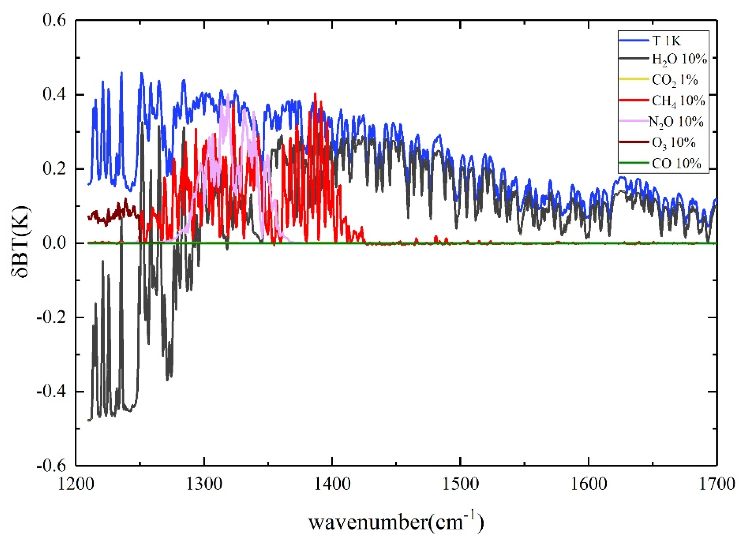
In the thermal infrared spectrum, the CH4 absorption band is located around 7.7 μm. Satellite observations in the spectral band are significantly affected by other atmospheric and surface parameters. In this section, the impact of variations in temperature, humidity profiles and in O3, CO2, CH4, N2O, and other gases on HIRAS radiance is calculated within 1200–1700 cm−1. The temperature and humidity profiles, ozone profiles, carbon dioxide, methane, nitrous oxide, and other gas profiles used in this study are derived from 80 globally representative thermodynamic initial guess retrieval (TIGR) [36] atmospheric profiles. The used data samples cover profile data from different seasons and latitudes. The radiance (or brightness temperature (BT)) is obtained by calculating these profiles in the sample set through the forward fast radiative transfer model, RTTOV. Figure 2 illustrates the average variations in HIRAS BT corresponding with the changes of 10% CH4, 10% CO, 10% N2O, 10% O3, 10% H2O, 1 K T, and 1% CO2. From Figure 2, it can be concluded that the variation in HIRAS BT at the methane absorption band of 7.7 μm (approximately 1299 cm−1) is influenced not only by changes in methane but also by variations in temperature and humidity profiles and N2O. The changes in other gases have minimal impact on HIRAS BT in this spectral region. Therefore, the key issue is how to extract more methane information from these bands while avoiding interference from N2O and temperature/humidity variations.
The key purpose of channel selection is to maximize the retrieval accuracy. Currently, those employed methods, for example the Jacobian method, and information entropy iterative method are used to study suitable numerical methods for selecting channels that are sensitive to atmospheric parameter inversion. These methods consider the channel’s sensitivity to atmospheric parameters, channel noise, background covariance matrix, and other factors. The selection criteria vary depending on the specific focus. The methane absorption bands are affected by gases such as water vapor and N2O. To avoid selecting channels with significant water vapor information for retrieval, this study adopts the Jacobian matrix peak method for channel selection.
The sensitivity of each channel to atmospheric components at corresponding altitude levels can be expressed by Jacobian matrix. This is defined as follows:
where xCH4 represents the CH4, and F(x) represents the forward radiative transfer model RTTOV with respect to state vector x. In this study, the Jacobian for CH4 is calculated by RTTOV.
The Jacobian matrix peak method was used to select CH4 profile retrieval channels. For each pressure level, the channel with the maximum ratio of peak value to width in the Jacobian matrix was chosen. The width of the Jacobian matrix was defined as the square root of the sum of the absolute values of all elements in the corresponding column vector [37].
The Jacobian for CH4 was calculated using the 80 globally representative atmospheric profiles from the TIGR database. The selected atmospheric profile samples were from TIGR, The geographical extent ranges from 70°S to 70°N. In the text, these profiles are classified into four categories: high latitude between 90°S–30°S and 30–90°N in autumn and winter (HW), high latitude between 90°S–30°S and 30–90°N in spring and summer (HS), low latitude (30°S–30°N) in autumn and winter (LW), and low latitude (30°S–30°N) in spring and summer (LS). Figure 3 illustrates the average Jacobian of CH4 absorption spectral bands (1210 to 1370 cm−1) calculated by RTTOV for the four scenarios mentioned above. It can be observed that the sensitivity of CH4 peaks occurred in the middle-to-upper troposphere, and that the distribution of CH4 Jacobian matrices varied among the four scenarios. This discrepancy is attributed to significant differences across different regions and seasons of temperature and H2O.
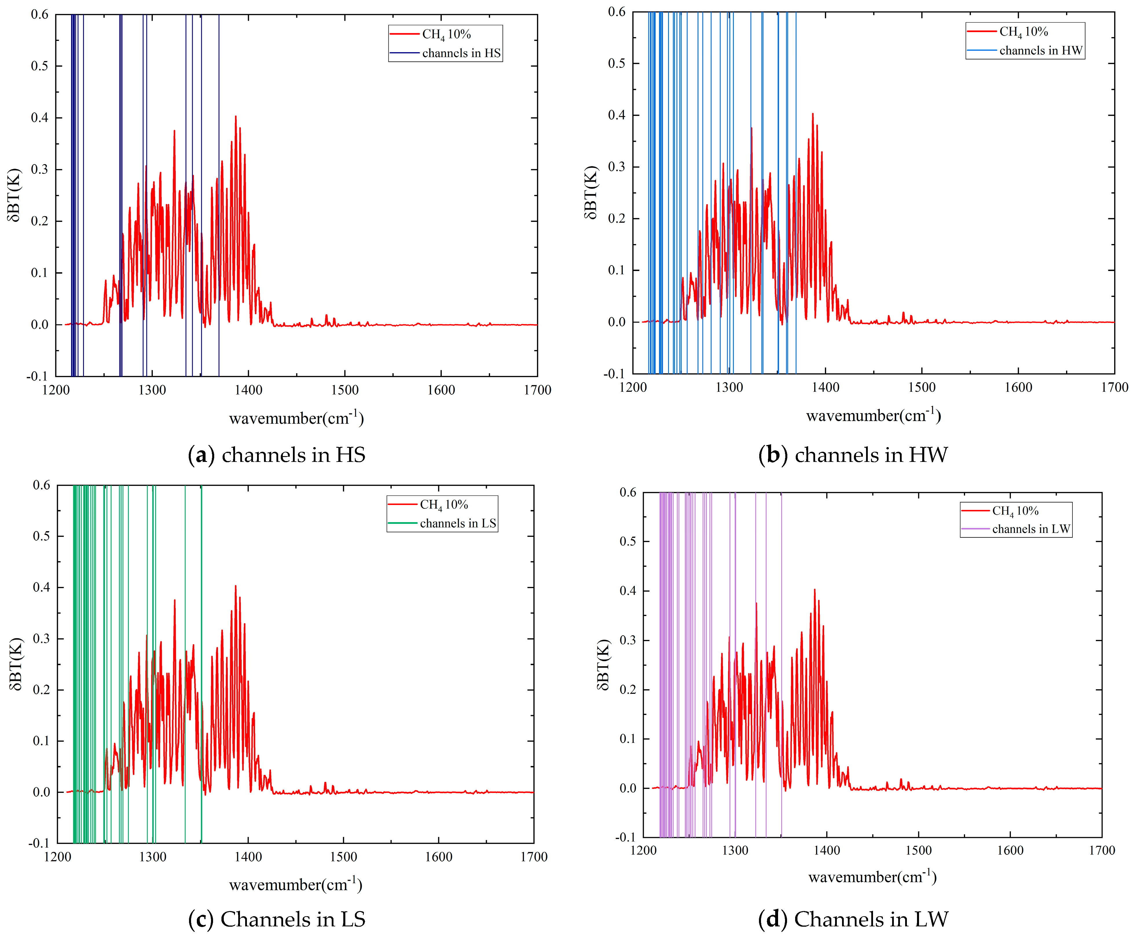
Considering the Jacobian matrix for methane, the impact on simulated satellite radiance and the redundancy information near 7.7 μm, the CH4 retrieval channels were selected which exhibited high sensitivity to CH4 but maintained relative insensitivity to other disturbances. In LS, a set of 36 channels was designated for CH4 profile inversion, where the greatest values of the CH4 Jacobian matrix were observed at the range of 100–200 hPa. In HS, 26 channels were selected for CH4 inversion, and the greatest value of the CH4 Jacobian matrix occurred from 300 to 400 hPa. In LW, 36 channels were selected for CH4 inversion, and the greatest value of the CH4 Jacobian matrix occurred from 300 to 400 hPa. In HW, 34 channels were selected for CH4 inversion, and the greatest value of the CH4 Jacobian matrix occurred from 400 to 500 hPa. Figure 4 shows the retrieved channels in different scenarios near the CH4 absorption bands.
3.2. Retrieval Algorithm
In this paper, the optimization method was adopted to retrieve the CH4 profile. The cost function can be expressed in Equation (2). The optimization method was used to minimize the cost function. The singular value decomposition (SVD) algorithm [29] is adopted to acquire the optimal estimation Xmethane. The simplified formula can be expressed in Equation (3) [37]:
where y is the satellite observed radiance with a total cloud cover of less than 30%, F(X,b) is the radiance calculated by RTTOV, X is the retrieved parameter, Xpriori is the CH4 first-guess profile, R−1 is the error covariance matrix of satellite observation, B−1 is the inverse covariance of the a priori Xpriori, C represents the conversion matrix, E represents the eigenvalue diagonal matrix, J is the Jacobian matrix, and Xpriori is the CH4 first-guess profile [37]. In this work, the clear-sky radiance of HIRAS y was derived using the cloud product from MERSI, and F(Xpriori) is the simulated radiance which was computed by RTTOV.
The empirical orthogonal functions (EOF) algorithm was applied to compute CH4 a priori state vector Xpriori. The method involved two steps: training and application. Firstly, the atmospheric parameter vertical profiles and corresponding satellite radiances were simultaneously represented as linear combinations of empirical orthogonal functions, calculating regression coefficients. Then, the inversion was performed using the obtained regression coefficients [37]. The atmospheric vertical profile samples applied in the method were obtained from ECMWF observational samples based on radio sounding data. Approximately 80 atmospheric profiles samples were used from the entire dataset, covering various seasons, latitudes, and geographical locations between 70°N and 70°S. These CH4 samples were extracted from experiments conducted by the ECMWF as part of the global and regional earth-system monitoring using satellite and in-situ data (GEMS) project [38]. The parameters P and R in Equation (3) represent the atmospheric composition profiles and the simulated radiance (or brightness temperature), respectively. R was calculated through the RTTOV model based on the band response functions of HIRAS and the profiles. Finally, based on representative atmospheric constituent profiles and corresponding simulated observational data, we obtained a training set for statistical regression. The variation in the observation zenith angle is also affected due to the longer path for the channels on the absorption bands. To avoid errors in the inversion process due to solar angles, R was computed at various observation zenith angles and incident zenith angles ranging from 0° to 70° with a 5° interval.
During the calculation process, regression coefficient matrices S were generated for different viewing angles [22]. The a priori CH4 profile can be expressed in Equation (4).
where represents the average of selected profile samples; meanwhile, is the difference matrix computed through the observed radiance and the averaged simulated radiance samples.
In the inversion process, the atmospheric temperature, humidity, and ozone profiles data input to the RTTOV model were derived from European Centre for Medium-Range Weather Forecasts (ECMWF) Re-analysis v5 (ERA5) data. The high-precision reanalysis ERA5 data were characterized by an hourly temporal resolution and a spatial resolution of 0.25° × 0.25° (https://www.ecmwf.int/, accessed on 5 June 2023). In this paper, the simulated radiancesRTTOV or BTRTTOV were obtained by inputting the relevant data of ERA5, HIRAS, solar geographic information, and the first-guess profile of CH4 into RTTOV model.
4. Results
4.1. Validation with CARIBIC
To validate the accuracy of the HIRAS CH4 retrieval, the retrieved HIRAS CH4 profiles are compared with CARIBIC observational profiles. As HIRAS data became available as of January 2019, we selected CARIBIC flight data from 2019 onwards for comparison. Based on the data provided on the official CARIBIC website, we selected four days of 10 s averaged flight data that met our requirements (as described in Section 2.3). The selected flights data covered a pressure range of 200 to 700 hPa. To align the spatial resolution of CARIBIC with satellite data, the CARIBIC CH4 profiles were averaged along the flight track at 0.25° intervals. Considering the differences in the CH4 weighting function distribution of HIRAS, the comparison was divided into two parts: mid latitudes from 30°N to 60°N and high latitudes from 60°N to 90°N. It is important to consider the diverse vertical resolutions when making significant comparisons with the retrieved CH4 profiles, so an averaging kernel (AK) matrix was applied to smooth the CH4 profiles of CARIBIC [37,39]. The smoothed CH4 measurements were then compared with the HIRAS profiles. The smoothed CARIBIC CH4 profiles can be obtained through the following procedure:
where Xobserved represents the CH4 observation profiles from CARIBIC.
It can be concluded that the correlation coefficients between the HIRAS CH4 profiles and the smoothed CARIBIC observational profiles were greater than 0.6 in Figure 5. Table 2 provides detailed information on the correlation coefficient (r), root mean square error (RMSE), and relative difference (RD) between the HIRAS CH4 profiles and the smoothed CARIBIC CH4 profiles. The relative difference is defined as follows:
As shown in Table 2, the correlation coefficients (r) between the HIRAS CH4 profiles and the CARIBIC observational profiles were slightly higher in low-latitude regions than in mid-latitude regions, with slightly smaller relative difference (RD) and root mean square error (RMSE) values. The RD values were 0.03–0.04% and less than 0.11% in low-latitude and mid-latitude regions, respectively. The maximum and minimum RMSE values in the low-latitude region were 21.2 ppbv and 8.9 ppbv, respectively. In the mid-latitude region, the maximum and minimum RMSE values were 30 ppbv and 19 ppbv, respectively. This could be attributed to the relatively lower CH4 concentrations in high-latitude regions, and the influence of temperature and water vapor.
4.2. Validation with FTIR
In this section, we compare the CH4 profiles measured by FTIR and HIRAS. Table 1 provides detailed information on FTIR sites, including the geographic coordinates, time ranges, and the altitude of the sites. To keep enough data and ensure consistency in dimension, the HIRAS L1 data that matched to the FTIR sites were resampled using a 0.25° x 0.25° grid resolution. Because FTIR and HIRAS measurement results have different vertical resolutions, comparing measurements directly from different data sources was an unsound practice. In this section, we used the retrieved Aks to obtain the smoothed FTIR CH4 profiles. The smoothed FTIR CH4 profiles can be obtained through Formula (4), in which Xobserved represents the FTIR observation profile. The CH4 profile of FTIR was processed into 101 layers, which was the same number as with the retrieved CH4 profiles’ layers.
Figure 6 shows the CH4 profiles (a priori, retrieved, and smoothed) and error distribution. The pink solid line, light green solid line, and light blue solid line represent the mean a priori, smoothed, and inverted profiles, respectively, while the shaded areas represent the standard deviation of each item. It can be observed that the CH4 inverted profiles exhibited larger standard deviations between 10–100 hPa compared with 100–1000 hPa, particularly at the St. Petersburg, Toronto, Rikubutsu, Altzomoni, and Wollongong sites. The errors between the a priori and retrieved values, as well as between the retrieved and smoothed values, were larger around 400–500 hPa. However, the errors between the retrieved and smoothed values were smaller compared with the errors between the a priori and smoothed values. Specifically, the errors between the retrieved and smoothed CH4 profiles were <100 ppbv at the St. Petersburg site, <50 ppbv at the Bremen site, <120 ppbv at the Toronto site, <62 ppbv at the Rikubutsu site, <52 ppbv at the Altzomoni site, and <45 ppbv at the Wollongong site.
Figure 7 shows the average column Aks (The sum of each AK column is referred to as the “area of AK” or “verticality.”) corresponding with the retrieved CH4 profiles at FTIR sites in different seasons. To calculate the inversion results of AKs for different seasons, sample sizes for each season were only counted if they exceeded five days. It can be observed that the maximum sensitivity often took place during the summer months (e.g., the peaks of Aks for St. Petersburg, Bremen, Rikubetsu, and Wollongong are in summer), while the peak sensitivity for the Toronto and Altzomoni sites occurred in autumn and spring, respectively. It can also be concluded that the majority of the greatest values of the average column averaging kernels exceed 1.5, except for the Altzomoni site, where they were almost all below 1.5. This could be influenced by the latitude and the temperature and humidity profiles, with a greater impact of temperature and humidity resulting in higher peak values of the average column averaging kernels. In the case of mid-latitude regions between 30°N and 60°N, the layer exhibiting peak sensitivity was approximately at 300–400 hPa, while for the low latitudes spanning from 0°N to 30°N, this sensitive layer tended to be at 200–300 hPa. The vertical sensitivity of CH4 inversion exhibited geographical and seasonal variations. Additionally, the distributions of CH4 AKs indicate how the a priori profile affected the inverted profile. The higher sensitivity in the mid-to-upper troposphere indicates that HIRAS can better retrieve CH4 within this range, while the lower sensitivity at the surface suggests that the CH4 profiles at these altitudes from HIRAS primarily rely on a priori information.
4.3. Uncertainty Analysis
From Figure 2, it is evident that, near the methane absorption band, the retrieval is influenced by temperature and humidity profiles as well as by variations in N2O. To avoid the influence of N2O, when selecting methane retrieval channels, N2O absorption channels are avoided. Therefore, the main sources of error in methane retrieval include the impacts of the temperature and H2O profiles input into the RTTOV model. The temperature and humidity profiles used in this study were sourced from ERA5 data. In the troposphere and lower stratosphere, from 1000 hPa to 10 hPa, the temperature errors are less than 0.2 K, but the errors are larger in 10 hPa to 1 hPa, where they are typically around ~2 K. The percentage errors of ERA5 humidity are around ~5%. Therefore, considering the precision of ERA5 temperature and H2O profiles, this section conducted an uncertainty analysis of the methane retrieval accuracy using temperature and H2O profiles from one mid-latitude and one low-latitude FTIR site (Rikubetsu and Altzomoni sites, respectively), coupled with a 5% variability in the H2O profile. In these sites, the temperature profile changed by 0.2 K from 1000 to 10 hPa, and a 2 K difference from 10 to 1 hPa.
Figure 8 illustrates the variations in retrieved CH4 profiles with respect to the smoothed profiles at the Altzomoni and Rikubetsu sites due to changes in temperature and water vapor. The red color (“origin”) represents the error between the methane retrieval results and the smoothed profile when temperature and humidity profiles remain unchanged, while the black color (“H2O”) represents the error when the water vapor profile changes by 5%. The blue color (“T”) indicates the error when the temperature profile changes by 0.2 K from 1000 to 10 hPa and a 2 K difference from 10 to 1 hPa. The green color (“H2O + T”) represents the error when both the water vapor profile changes by 5% and the temperature profile changes as described above. The results show that the error in methane profile changes due to a 5% variation in water vapor profile was slightly higher than the error caused by temperature profile changes at the Altzomoni and Rikubetsu sites. The error in methane profile changes due to simultaneous variations in temperature and humidity profiles (“H2O + T”) was as follows: the maximum error is around 79 ppbv at around 500 hPa, with an average error of 32.2 ppbv and a standard deviation of 43.6 ppbv for the entire profile at Altzomoni site, and the maximum error is around 95.4 ppbv at around 470 hPa, with an average error of 33.3 ppbv and a standard deviation of 27.3 ppbv for the entire profile at Rikubetsu site.
5. Discussion
This paper selected different methane retrieval channels based on CH4 Jacobians for different latitudes and seasons, as outlined in Section 3.1. In this subsection, we respectively changed the retrieval channels at Altzomoni and Rikubetsu sites, and then compared the retrieval results with the unchanged channels’ results, described in Section 4.2. The Altzomoni site is located at a low-latitude region, and channels from high-latitude regions were used for Altzomoni retrieval. The retrieval channels at Rikubetsu were exchanged according to the season, with channels from autumn and winter used in spring and summer, and channels from spring and summer used in autumn and winter (as shown in Figure 9). It can be observed that, after changing the inversion channels, the errors between the retrieval results and the observed values from smoothed FTIR measurements significantly increased at Altzomoni. The methane retrieval errors at Altzomoni, without changing the channels, were 19.2, 30.8, 23.3, and 15.9 ppbv for spring, summer, autumn, and winter, respectively. After changing the channels, the methane retrieval errors were 38.2, 54.1, 35.9, and 41 ppbv, respectively. Similarly, the errors between the retrieval results and the observed values from smoothed FTIR measurements also increased significantly at Rikubetsu. The methane retrieval errors at Rikubetsu, without changing the channels, were 73.2, 23, and 12 ppbv for spring, summer, and autumn, respectively. After changing the channels, the methane retrieval errors were 66.2, 34.8, and 19.8 ppbv, respectively. Finally, it is revealed that the retrieval accuracy can be improved by using latitude and seasonal retrieval channels selection.
6. Conclusions
The paper utilized the FY3D HIRAS L1 radiance product from the China National Satellite Meteorological Center, and employed cloud products from FY3D MERSI for cloud screening, to retrieve methane profiles. Section 3 introduced the retrieval method of methane profile in detail and the selection of methane retrieval channels. The paper obtained the methane retrieval channels under four different scenarios of HS, HW, LS and LW, based on the distribution of a methane Jacobian matrix at different latitudes and seasons. CH4 Jacobians showed that the sensitivity reached a peak in higher altitudes for LS and lower altitudes for HW. Then, we compared the retrieved HIRAS CH4 profiles with CARIBIC and FTIR observational profiles to validate the accuracy of the HIRAS CH4 profile inversion. Compared with CARIBIC, the results show that the averaged correlation coefficients, relative difference and root mean square error were 0.73, 0.0491 and 18.9 ppbv, respectively, and that the relative differences and root mean square errors in the low-latitude region were lower than those in the mid-latitude region. It can be observed that the CH4 inverted profiles in FTIR stations exhibited larger standard deviations between 10–100 hPa compared with 100–1000 hPa. The errors between the a priori and retrieved values, as well as between the retrieved and smoothed values, were larger around 400–500 hPa. Sensitivity peaks were mainly observed during the summer season. However, Toronto experienced its peak in the fall, and Altzomoni experienced its peak in the spring. It is observed that the greatest values of the average column-averaged kernels typically surpass 1.5. Overall, the methane profile retrieval results based on the HIRAS L1 product can serve as a reference for the distribution of atmospheric methane.
Author Contributions
Conceptualization, X.Z. and Y.Z.; methodology, Y.Z. and L.C.; software, Y.Z.; validation, X.Z.; formal analysis, X.Z., Y.Z. and F.M.; investigation, X.Z. and H.W.; resources, J.T. and Y.W.; data curation, X.Z.; writing—original draft, X.Z.; writing—review and editing, X.Z., and F.M.; visualization, X.Z.; supervision, Y.Z. and F.M.; project administration, Y.Z. and L.C.; funding acquisition, L.C., F.M.,Y.Z. and X.Z. All authors have read and agreed to the published version of the manuscript.
Funding
This study was supported by the National Key Research and Development Program of China (Grant No. 2022YFB3904801), Open Foundation of State Key Laboratory of Remote Sensing Science of China (OFSLRSS202211, OFSLRSS202203), National Natural Science Foundation of China (42201375, 41901269), Fengyun Application Pioneering Project (FY-APP-2022.0501).
Data Availability Statement
The Hyperspectral Infrared Atmospheric Sounder (HIRAS) level 1 Data and Medium Resolution Spectral imager (MERSI) cloud products from the National Satellite Meteorological Center of China can be found at https://satellite.nsmc.org.cn/PortalSite/Data/Satellite.aspx?currentculture=zh-CN (accessed on 15 June 2023); The Civil Aircraft for the Regular Investigation of the Atmosphere Based on an Instrument Container (CARIBIC) can be found at http://www.caribic-atmospheric.com/ (accessed on 28 November 2022); the European Centre for Medium-Range Weather Forecasts (ECMWF) Reanalysis v5 (ERA5) can be found at https://www.ecmwf.int/en/forecasts/datasets/reanalysis-datasets/era5 (accessed on 5 June 2023); the Fourier transform infrared spectrometer (FTIR) data of the Infrared Working Group (IRWG) of the Network for the Detection of Atmospheric Composition Change (NDACC) can be found at https://ndacc.larc.nasa.gov/data (accessed on 23 November 2022).
Acknowledgments
We would like to express our thanks to the following organizations for providing data to this research: The HIRAS level 1 Data and MERSI cloud product were developed by the National Satellite Meteorological Center of China. The CARIBIC data was supported by IAGOS CARIBIC Community. ERA5 reanalysis data was provided by ECMWF. The FTIR data was provided by NDACC.
Conflicts of Interest
The authors declare no conflicts of interest.
References
- Bousquet, P.; Ciais, P.; Miller, J.B.; Dlugokencky, E.J.; Hauglustaine, D.A.; Prigent, C.; Van der Werf, G.R.; Peylin, P.; Brunke, E.G.; Carouge, C.; et al. Contribution of anthropogenic and natural sources to atmospheric methane variability. Nature 2006, 443, 439–443. [Google Scholar] [CrossRef]
- Friedlingstein, P.; O’Sullivan, M.; Jones, M.W.; Andrew, R.M.; Gregor, L.; Hauck, J.; Le Quéré, C.; Luijkx, I.T.; Olsen, A.; Peters, G.P.; et al. Global Carbon Budget 2022. Earth Syst. Sci. Data 2022, 14, 4811–4900. [Google Scholar] [CrossRef]
- Peng, S.; Piao, S.; Bousquet, P.; Ciais, P.; Li, B.; Lin, X.; Tao, S.; Wang, Z.; Zhang, Y.; Zhou, F. Inventory of anthropogenic methane emissions in China’s mainland from 1980 to 2010. Atmos. Chem. Phys. 2016, 16, 14545–14562. [Google Scholar] [CrossRef]
- Saunois, M.; Stavert, A.R.; Poulter, B.; Bousquet, P.; Canadell, J.G.; Jackson, R.B.; Raymond, P.A.; Dlugokencky, E.J.; Houweling, S.; Patra, P.K.; et al. The Global Methane Budget 2000–2017. Earth Syst Sci Data 2020, 12, 1561–1623. [Google Scholar] [CrossRef]
- Wuebbles, D.J.; Hayhoe, K. Atmospheric methane and global change. Earth Sci. Rev. 2002, 57, 177–210. [Google Scholar] [CrossRef]
- Sepúlveda, E.; Schneider, M.; Hase, F.; García, O.E.; Gomez-Pelaez, A.; Dohe, S.; Blumenstock, T.; Guerra, J.C. Long-term validation of tropospheric column-averaged CH4 mole fractions obtained by mid-infrared ground-based FTIR spectrometry. Atmos. Meas. Tech. 2012, 5, 1425–1441. [Google Scholar] [CrossRef]
- Sha, M.K.; Langerock, B.; Blavier, J.F.L.; Blumenstock, T.; Borsdorff, T.; Buschmann, M.; Dehn, A.; De Mazière, M.; Deutscher, N.M.; Feist, D.G.; et al. Validation of methane and carbon monoxide from Sentinel-5 Precursor using TCCON and NDACC-IRWG stations. Atmos. Meas. Tech. 2021, 14, 6249–6304. [Google Scholar] [CrossRef]
- Buchholz, R.R.; Deeter, M.N.; Worden, H.M.; Gille, J.; Edwards, D.P.; Hannigan, J.W.; Jones, N.B.; Paton-Walsh, C.; Griffith, D.W.T.; Smale, D.; et al. Validation of MOPITT carbon monoxide using ground-based Fourier transform infrared spectrometer data from NDACC. Atmos. Meas. Tech. 2017, 10, 1927–1956. [Google Scholar] [CrossRef]
- Barret, B.; Gouzenes, Y.; Le Flochmoen, E.; Ferrant, S. Retrieval of Metop-A/IASI N2O Profiles and Validation with NDACC FTIR Data. Atmosphere 2021, 12, 219. [Google Scholar] [CrossRef]
- García, O.E.; Sanromá, E.; Schneider, M.; Hase, F.; León-Luis, S.F.; Blumenstock, T.; Sepúlveda, E.; Redondas, A.; Carreño, V.; Torres, C.; et al. Improved ozone monitoring by ground-based FTIR spectrometry. Atmos. Meas. Tech. 2022, 15, 2557–2577. [Google Scholar] [CrossRef]
- Brenninkmeijer, C.A.M.; Crutzen, P.; Boumard, F.; Dauer, T.; Dix, B.; Ebinghaus, R.; Filippi, D.; Fischer, H.; Franke, H.; Friess, U.; et al. Civil Aircraft for the regular investigation of the atmosphere based on an instrumented container: The new CARIBIC system. Atmos. Chem. Phys. 2007, 7, 4953–4976. [Google Scholar] [CrossRef]
- De Wachter, E.; Kumps, N.; Vandaele, A.C.; Langerock, B.; De Mazière, M. Retrieval and validation of MetOp/IASI methane. Atmos. Meas. Tech. 2017, 10, 4623–4638. [Google Scholar] [CrossRef]
- Zhang, L.J.; Wei, C.; Liu, H.; Jiang, H.; Lu, X.H.; Zhang, X.Y.; Jiang, C. Comparison analysis of global methane concentration derived from SCIAMACHY, AIRS, and GOSAT with surface station measurements. Int. J. Remote Sens. 2021, 42, 1823–1840. [Google Scholar] [CrossRef]
- Fu, D.; Bowman, K.W.; Worden, H.M.; Natraj, V.; Worden, J.R.; Yu, S.; Veefkind, P.; Aben, I.; Landgraf, J.; Strow, L.; et al. High-resolution tropospheric carbon monoxide profiles retrieved from CrISand TROPOMI. Atmos. Meas. Tech. 2016, 9, 2567–2579. [Google Scholar] [CrossRef]
- Wu, C.Q.; Qi, C.L.; Hu, X.Q.; Gu, M.J.; Yang, T.H.; Xu, H.L.; Lee, L.; Yang, Z.D.; Zhang, P. FY-3D HIRAS Radiometric Calibration and Accuracy Assessment. IEEE Trans. Geosci. Remote 2020, 58, 3965–3976. [Google Scholar] [CrossRef]
- Noël, S.; Bramstedt, K.; Hilker, M.; Liebing, P.; Plieninger, J.; Reuter, M.; Rozanov, A.; Sioris, C.E.; Bovensmann, H.; Burrows, J.P. Stratospheric CH4 and CO2 profiles derived from SCIAMACHY solar occultation measurements. Atmos. Meas. Tech. 2016, 9, 1485–1503. [Google Scholar] [CrossRef]
- Wang, S.P.; van der A, R.J.; Stammes, P.; Wang, W.H.; Zhang, P.; Lu, N.M.; Zhang, X.Y.; Bi, Y.M.; Wang, P.; Fang, L. Carbon Dioxide Retrieval from TanSat Observations and Validation with TCCON Measurements. Remote Sens. 2020, 12, 3626. [Google Scholar] [CrossRef]
- Feng, L.; Palmer, P.I.; Bösch, H.; Parker, R.J.; Webb, A.J.; Correia, C.S.C.; Deutscher, N.M.; Domingues, L.G.; Feist, D.G.; Gatti, L.V.; et al. Consistent regional fluxes of CH4 and CO2 inferred from GOSAT proxy XCH4: XCO2 retrievals, 2010–2014. Atmos. Chem. Phys. 2017, 17, 4781–4797. [Google Scholar] [CrossRef]
- Das, C.; Kunchala, R.K.; Chandra, N.; Chhabra, A.; Pandya, M.R. Characterizing the regional XCO2 variability and its association with ENSO over India inferred from GOSAT and OCO-2 satellite observations. Sci. Total Environ. 2023, 902, 166176. [Google Scholar] [CrossRef] [PubMed]
- Gao, M.Z.; Xing, Z.Y.; Vollrath, C.; Hugenholtz, C.H.; Barchyn, T.E. Global observational coverage of onshore oil and gas methane sources with TROPOMI. Sci. Rep. 2023, 13, 16759. [Google Scholar] [CrossRef] [PubMed]
- Trieu, T.T.N.; Morino, I.; Uchino, O.; Tsutsumi, Y.; Sakai, T.; Nagai, T.; Yamazaki, A.; Okumura, H.; Arai, K.; Shiomi, K.; et al. Influences of aerosols and thin cirrus clouds on GOSAT XCO2 and XCH4 using Total Carbon Column Observing Network, sky radiometer, and lidar data. Int. J. Remote Sens. 2022, 43, 1770–1799. [Google Scholar] [CrossRef]
- Zhang, Y.; Xiong, X.; Tao, J.; Yu, C.; Zou, M.; Su, L.; Chen, L. Methane retrieval from Atmospheric Infrared Sounder using EOF-based regression algorithm and its validation. Chin. Sci. Bull. 2014, 59, 1508–1518. [Google Scholar] [CrossRef]
- Xiong, X.; Barnet, C.; Maddy, E.; Sweeney, C.; Liu, X.; Zhou, L.; Goldberg, M. Characterization and validation of methane products from the Atmospheric Infrared Sounder (AIRS). J. Geophys. Res. Biogeosci. 2008, 113, G3. [Google Scholar] [CrossRef]
- Crevoisier, C.; Nobileau, D.; Fiore, A.M.; Armante, R.; Chédin, A.; Scott, N.A. Tropospheric methane in the tropics—First year from IASI hyperspectral infrared observations. Atmos. Chem. Phys. 2009, 9, 6337–6350. [Google Scholar] [CrossRef]
- Nalli, N.R.; Tan, C.Y.; Warner, J.; Divakarla, M.; Gambacorta, A.; Wilson, M.; Zhu, T.; Wang, T.Y.; Wei, Z.G.; Pryor, K.; et al. Validation of Carbon Trace Gas Profile Retrievals from the NOAA-Unique Combined Atmospheric Processing System for the Cross-Track Infrared Sounder. Remote Sens. 2020, 12, 3245. [Google Scholar] [CrossRef]
- Li, H.; Gu, M.; Zhang, C.; Xie, M.; Yang, T.; Hu, Y. Retrieving Atmospheric Gas Profiles Using FY-3E/HIRAS-II Infrared Hyperspectral Data by Neural Network Approach. Remote Sens. 2023, 15, 2931. [Google Scholar] [CrossRef]
- Turquety, S.; Hadji-Lazaro, J.; Clerbaux, C.; Hauglustaine, D.A.; Clough, S.A.; Cassé, V.; Schlüssel, P.; Mégie, G. Operational trace gas retrieval algorithm for the Infrared Atmospheric Sounding Interferometer. J. Geophys. Res. Atmos. 2004, 109, D21. [Google Scholar] [CrossRef]
- Rodgers, C.D. Retrieval of Atmospheric-Temperature and Composition from Remote Measurements of Thermal-Radiation. Rev. Geophys. 1976, 14, 609–624. [Google Scholar] [CrossRef]
- Susskind, J.; Barnet, C.D.; Blaisdell, J.M. Retrieval of atmospheric and surface parameters from AIRS/AMSU/HSB data in the presence of clouds. IEEE Trans. Geosci. Remote Sens. 2003, 41, 390–409. [Google Scholar] [CrossRef]
- Xu, N.; Niu, X.H.; Hu, X.Q.; Wang, X.H.; Wu, R.H.; Chen, S.S.; Chen, L.; Sun, L.; Ding, L.; Yang, Z.D.; et al. Prelaunch Calibration and Radiometric Performance of the Advanced MERSI II on FengYun-3D. IEEE Trans. Geosci. Remote 2018, 56, 4866–4875. [Google Scholar] [CrossRef]
- Zhang, X.; Shi, C.; Si, Y.; Letu, H.; Wang, L.; Tang, C.; Xu, N.; He, X.; Yin, S.; Zhang, Z.; et al. Remote Sensing of Aerosols and Water-Leaving Radiance from Chinese FY-3/MERSI Based on a Simultaneous Method. Remote Sens. 2023, 15, 5650. [Google Scholar] [CrossRef]
- Si, Y.D.; Chen, L.; Zheng, Z.J.; Yang, L.K.; Wang, F.; Xu, N.; Zhang, X.Y. A Novel Algorithm of Haze Identification Based on FY3D/MERSI-II Remote Sensing Data. Remote Sens. 2023, 15, 438. [Google Scholar] [CrossRef]
- Bell, B.; Hersbach, H.; Simmons, A.; Berrisford, P.; Dahlgren, P.; Horányi, A.; Muñoz-Sabater, J.; Nicolas, J.; Radu, R.; Schepers, D.; et al. The ERA5 global reanalysis: Preliminary extension to 1950. Q. J. Roy. Meteor. Soc. 2021, 147, 4186–4227. [Google Scholar] [CrossRef]
- Almeida, M.; Coelho, P. A first assessment of ERA5 and ERA5-Land reanalysis air temperature in Portugal. Int. J. Climatol. 2023, 43, 6643–6663. [Google Scholar] [CrossRef]
- Saunders, R.; Hocking, J.; Turner, E.; Rayer, P.; Rundle, D.; Brunel, P.; Vidot, J.; Roquet, P.; Matricardi, M.; Geer, A.; et al. An update on the RTTOV fast radiative transfer model (currently at version 12). Geosci. Model Dev. 2018, 11, 2717–2732. [Google Scholar] [CrossRef]
- Chevallier, F.; Chéruy, F.; Scott, N.A.; Chédin, A. A Neural Network Approach for a Fast and Accurate Computation of a Longwave Radiative Budget. J. Appl. Meteorol. 1998, 37, 1385–1397. [Google Scholar] [CrossRef]
- Zhang, X.X.; Zhang, Y.; Bai, L.; Tao, J.H.; Chen, L.F.; Zou, M.M.; Han, Z.F.; Wang, Z.B. Retrieval of Carbon Dioxide Using Cross-Track Infrared Sounder (CrIS) on S-NPP. Remote Sens. 2021, 13, 1163. [Google Scholar] [CrossRef]
- Marco, M. The Generation of RTTOV Regression Coefficients for IASI and Airs Using a New Profile Training Set and a New Line-by-Line Database; ECMWF Technical Memoranda: Reading, UK, 2008. [Google Scholar]
- Xiong, X.; Han, Y.; Liu, Q.; Weng, F. Comparison of Atmospheric Methane Retrievals From AIRS and IASI. IEEE J. Sel. Top. Appl. Earth Obs. Remote Sens. 2016, 9, 3297–3303. [Google Scholar] [CrossRef]
Figure 1.
Data from four flights of the Civil Aircraft for the Regular Investigation of the Atmosphere Based on an Instrument Container (CARIBIC). The light blue line is flight 569 (1 May 2019), the light green line is flight 575 (14 August 2019), the red line is flight 586 (9 January 2020), and the light pink line is flight 587 (10 January 2020).

Figure 2.
Sensitivities of HIRAS channels located in 1200−1750 cm−1 to variations of 1 K temperature (blue), 10% H2O (grey), 1% CO2 (yellow),10% CH4 (red), 10% N2O (pink), 10% O3 (dark red) and 10% CO (light blue).
Figure 2.
Sensitivities of HIRAS channels located in 1200−1750 cm−1 to variations of 1 K temperature (blue), 10% H2O (grey), 1% CO2 (yellow),10% CH4 (red), 10% N2O (pink), 10% O3 (dark red) and 10% CO (light blue).

Figure 3.
CH4 Jacobians (K/ppmv) from 1210 to 1400 cm−1 with a spectral resolution of 0.625 cm−1 for (a) high latitude between 90°S–30°S and 30–90°N in spring and summer (HS), (b) high latitude between 90°S–30°S and 30–90°N in spring and summer (HS), (c) low latitude (30°S–30°N) in spring and summer (LS) and (d) low latitude (30°S–30°N) in autumn and winter (LW). The different colors of the lines in the figure represent different channels (1210 to 1400 cm−1).

Figure 4.
CH4 retrieval channels in (a) HS, (b) HW (light blue line), (c) LS and (d) LW.

Figure 5.
CH4 comparison between HIRAS retrievals and smoothed CARIBIC with a 0.5° × 0.5° spatial resolution. (a) Flight no. 569, (b) flight no. 575, (c) flight no. 586, and (d) flight no. 587.
Figure 5.
CH4 comparison between HIRAS retrievals and smoothed CARIBIC with a 0.5° × 0.5° spatial resolution. (a) Flight no. 569, (b) flight no. 575, (c) flight no. 586, and (d) flight no. 587.

Figure 6.
CH4 profile comparisons between a priori (pink line), smoothing Fourier transform infrared spectrometer (FTIR) (light green line) observation products, and HIRAS retrieval (light blue line), in FTIR sites.
Figure 6.
CH4 profile comparisons between a priori (pink line), smoothing Fourier transform infrared spectrometer (FTIR) (light green line) observation products, and HIRAS retrieval (light blue line), in FTIR sites.

Figure 7.
The mean column averaging kernels of CH4 retrievals in FTIR stations. The blue, green, red, and black lines refer to spring, summer, autumn, and winter, respectively.
Figure 7.
The mean column averaging kernels of CH4 retrievals in FTIR stations. The blue, green, red, and black lines refer to spring, summer, autumn, and winter, respectively.

Figure 8.
Means of variations of CH4 induced by variations of T (1–10 hPa: 2 K; 10–1000 hPa: 0.2 K) and H2O (5%) in Altzomoni and Rikubetsu.
Figure 8.
Means of variations of CH4 induced by variations of T (1–10 hPa: 2 K; 10–1000 hPa: 0.2 K) and H2O (5%) in Altzomoni and Rikubetsu.

Figure 9.
Comparison of Altzomoni and Rikubetsu observations with inversion results (a) and inversion results using changed channels. (a) Channels in opposite seasons in Altzomoni and (b) channels in high latitudes in Rikubetsu.
Figure 9.
Comparison of Altzomoni and Rikubetsu observations with inversion results (a) and inversion results using changed channels. (a) Channels in opposite seasons in Altzomoni and (b) channels in high latitudes in Rikubetsu.


Table 1.
Detailed information of the selected Fourier transform infrared spectrometer (FTIR) stations used for CH4 retrieval validation.
Table 1.
Detailed information of the selected Fourier transform infrared spectrometer (FTIR) stations used for CH4 retrieval validation.
| Sites | Latitude | Longitude | Altitude (m) | Days | Start Date | End Date |
|---|---|---|---|---|---|---|
| St. Petersburg (Russia) | 59.88 | 29.83 | 20 | 109 | 1 May 2019 | 29 August 2021 |
| Bremen (Germany) | 53.1 | 8.8 | 27 | 81 | 1 May 2019 | 27 November 2020 |
| Toronto (Canada) | 43.66 | 79.36 | 174 | 238 | 5 May 2019 | 29 November 2020 |
| Rikubetsu (Japan) | 43.46 | 143.77 | 370 | 344 | 2 May 2019 | 29 September 2021 |
| Altzomoni (Mexico) | 19.1187 | −98.6552 | 3985 | 328 | 28 June 2019 | 30 May 2021 |
| Wollongong (Australia) | −34.41 | 150.88 | 30 | 225 | 8 June 2020 | 9 August 2021 |
Table 2.
CH4 comparisons between HIRAS and CARIBIC observations. The mean of the root mean square error (RMSE), relative difference (RD), correlation coefficient (r), and the number of grid cells (N).
Table 2.
CH4 comparisons between HIRAS and CARIBIC observations. The mean of the root mean square error (RMSE), relative difference (RD), correlation coefficient (r), and the number of grid cells (N).
| Date | Latitude | RMSE (ppbv) | RD (%) | r | N |
|---|---|---|---|---|---|
| 1 May 2019 | 30°N–60°N | 19 | 0.036 | 0.75 | 23 |
| 14 August 2019 | 30°N–60°N | 30 | 0.066 | 0.7 | 19 |
| 9 January 2020 | 30°S–60°N | 15.1 | 0.015 | 0.84 | 40 |
| 30°N–60°N | 19.2 | 0.08 | 0.2 | 10 | |
| 0°N–30°N | 16.7 | 0.04 | 0.63 | 15 | |
| 30°S–0°N | 8.9 | 0.03 | 0.74 | 15 | |
| 10 January 2020 | 0°N–60°N | 20.9 | 0.029 | 0.75 | 31 |
| 30°N–60°N | 19.3 | 0.108 | 0.66 | 8 | |
| 0°N–30°N | 21.2 | 0.0382 | 0.76 | 23 |
Disclaimer/Publisher’s Note: The statements, opinions and data contained in all publications are solely those of the individual author(s) and contributor(s) and not of MDPI and/or the editor(s). MDPI and/or the editor(s) disclaim responsibility for any injury to people or property resulting from any ideas, methods, instructions or products referred to in the content. |
© 2024 by the authors. Licensee MDPI, Basel, Switzerland. This article is an open access article distributed under the terms and conditions of the Creative Commons Attribution (CC BY) license (https://creativecommons.org/licenses/by/4.0/).
Share and Cite
MDPI and ACS Style
Zhang, X.; Zhang, Y.; Meng, F.; Tao, J.; Wang, H.; Wang, Y.; Chen, L. Methane Retrieval from Hyperspectral Infrared Atmospheric Sounder on FY3D. Remote Sens. 2024, 16, 1414. https://doi.org/10.3390/rs16081414
AMA Style
Zhang X, Zhang Y, Meng F, Tao J, Wang H, Wang Y, Chen L. Methane Retrieval from Hyperspectral Infrared Atmospheric Sounder on FY3D. Remote Sensing. 2024; 16(8):1414. https://doi.org/10.3390/rs16081414
Chicago/Turabian StyleZhang, Xinxin, Ying Zhang, Fan Meng, Jinhua Tao, Hongmei Wang, Yapeng Wang, and Liangfu Chen. 2024. "Methane Retrieval from Hyperspectral Infrared Atmospheric Sounder on FY3D" Remote Sensing 16, no. 8: 1414. https://doi.org/10.3390/rs16081414
Note that from the first issue of 2016, this journal uses article numbers instead of page numbers. See further details here.