
Time–Frequency Signal Integrity Monitoring Algorithm Based on Temperature Compensation Frequency Bias Combination Model

1
College of Electronic Science and Technology, National University of Defense Technology (NUDT), Changsha 410073, China
2
Key Laboratory of Satellite Navigation Technology, Changsha 410073, China
*
Author to whom correspondence should be addressed.
Remote Sens. 2024, 16(8), 1453; https://doi.org/10.3390/rs16081453
Submission received: 22 February 2024
/
Revised: 16 April 2024
/
Accepted: 17 April 2024
/
Published: 19 April 2024
Abstract
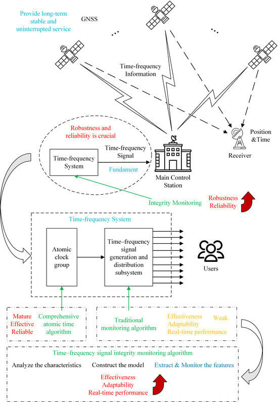
:To ensure the long-term stable and uninterrupted service of satellite navigation systems, the robustness and reliability of time–frequency systems are crucial. Integrity monitoring is an effective method to enhance the robustness and reliability of time–frequency systems. Time–frequency signals are fundamental for integrity monitoring, with their time differences and frequency biases serving as essential indicators. These indicators are influenced by the inherent characteristics of the time–frequency signals, as well as the links and equipment they traverse. Meanwhile, existing research primarily focuses on only monitoring the integrity of the time–frequency signals’ output by the atomic clock group, neglecting the integrity monitoring of the time–frequency signals generated and distributed by the time–frequency signal generation and distribution subsystem. This paper introduces a time–frequency signal integrity monitoring algorithm based on the temperature compensation frequency bias combination model. By analyzing the characteristics of time difference measurements, constructing the temperature compensation frequency bias combination model, and extracting and monitoring noise and frequency bias features from the time difference measurements, the algorithm achieves comprehensive time–frequency signal integrity monitoring. Experimental results demonstrate that the algorithm can effectively detect, identify, and alert users to time–frequency signal faults. Additionally, the model and the integrity monitoring parameters developed in this paper exhibit high adaptability, making them directly applicable to the integrity monitoring of time–frequency signals across various links. Compared with traditional monitoring algorithms, the algorithm proposed in this paper greatly improves the effectiveness, adaptability, and real-time performance of time–frequency signal integrity monitoring.
1. Introduction
The integrity of the time–frequency system is a critical determination of the navigation, positioning, and timing service performance of the Global Navigation Satellite System (GNSS). A fault within this system can inflict substantial damage on the GNSS operations. On 11 July 2019, a malfunction in the ground time–frequency system led to a disruption in the Galileo satellite navigation system. This incident affected over 20 satellites, resulting in the unavailability of navigation signals and a subsequent interruption of navigation, positioning, and timing services. These were not restored until a week later, significantly impacting both system operations and user services. To maintain the long-term stability and continuous service of satellite navigation systems, the robustness and reliability of time–frequency systems are essential. Integrity monitoring is a key strategy for enhancing these aspects. Therefore, there is an urgent need to conduct comprehensive research into the integrity monitoring of time–frequency systems to ensure the dependable functioning of the GNSS worldwide.
Currently, the development and research of integrity monitoring are primarily focused on the field of GNSS integrity monitoring, which is mainly divided into GNSS system integrity monitoring and receiver autonomous integrity monitoring (RAIM). The scope of GNSS system integrity monitoring is expansive, encompassing satellite integrity monitoring for satellite-based augmentation systems [1], real-time integrity monitoring for wide-area-precision positioning systems [2], and the theoretical framework for multi-tiered autonomous integrity monitoring in multi-source PNT elastic fusion navigation systems [3,4]. RAIM enables GNSS receivers to autonomously detect and rectify errors using redundant GNSS data. Scholars are presently delving into its methodological principles and performance analyses [5,6,7,8], availability and integrity risk assessment [9,10,11], GNSS satellite selection strategy [12], scenarios involving multiple constellations and faults [8,13,14,15], cross-integration with other disciplines [16], and applications in aviation, Precise Point Positioning (PPP), Real-Time Kinematics (RTK), and other fields [17,18,19,20,21,22]. In response to the integrity monitoring requirements of timing receivers with precisely known, stationary antenna coordinates, a Timing-Receiver Autonomous Integrity Monitoring (T-RAIM) algorithm has been proposed [23,24,25]. In order to meet the integrity monitoring needs of the aviation LPV-200 operation, an advanced receiver autonomous integrity monitoring (ARAIM) algorithm has been developed on the basis of the RAIM algorithm, and its performance is evaluated [26,27,28]. In addition, the receiver solution information combines external auxiliary information to develop an auxiliary integrity monitoring algorithm, which is mainly combined with auxiliary information such as inertial navigation, WIFI, and differential GNSS [29,30,31,32,33].
However, in the realm of time–frequency systems’ integrity monitoring, the time–frequency signal serves as the fundamental basis, with its time differences and frequency biases being important indicators for the assessment of the integrity monitoring of time–frequency systems. A typical time–frequency system is shown in Figure 1.
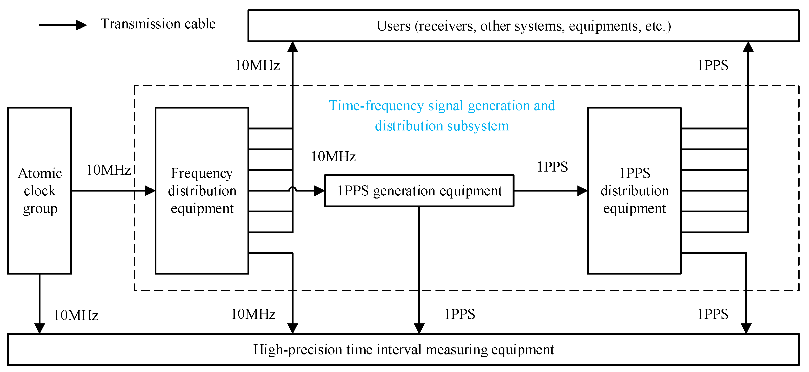
The time–frequency signal is generated by the time–frequency source in the atomic clock group, and is finally output to the users through a series of system equipment in the time–frequency system. All time–frequency signals in the time–frequency system are transmitted through cables. The 10 MHz frequency signal generated by the atomic clock group, after the time–frequency signal generation and distribution subsystem, generates multiple 10 MHz frequency signals and Pulse Per Second (1PPS) signals and outputs them to the users. Although the atomic clock group is the core part of the time–frequency system, the time–frequency signal generation and distribution subsystem is also an important part that affects the quality and performance of the time–frequency signal used by users. Therefore, to study the integrity monitoring of time–frequency systems, it is necessary to study the integrity monitoring of the time–frequency signals’ output by the atomic clock group and the time–frequency signal generation and distribution subsystem.
Presently, there is a scarcity of methods concerning the comprehensive monitoring of time–frequency signal integrity, particularly those emanating from the atomic clock ensemble within the time–frequency system. The existing approaches primarily involve cross-comparing the output signals of the atomic clocks, reviewing the phase, frequency deviation, and stability to achieve real-time integrity monitoring of the atomic clock’s signal output [34]. Current research only focuses on the integrity monitoring of the time–frequency signal produced by the atomic clock group, yet it neglects to monitor the integrity of the signals generated by the time–frequency signal generation and distribution subsystem.
In light of the aforementioned absence of integrity monitoring for the time–frequency signals generated by the time–frequency signal generation and distribution subsystem, this paper aims to explore the integrity monitoring of the time–frequency signals from the time–frequency signal generation and distribution subsystem. The structure of the article is as follows: Section 1 introduces the research background, significance, and current status of the integrity monitoring addressed in this article, along with proposing the research objectives. In Section 2, the characteristics of the measurement results between time–frequency signals are analyzed, a time–frequency signal temperature compensation frequency bias combination model is developed, and a time–frequency signal integrity monitoring algorithm along with its parameter calculation criteria based on the temperature compensation frequency bias combination model are proposed. Section 3 introduces the source of the time difference measurement results, which come from five different time–frequency signal links, and proposes experimental strategies. In Section 4, relevant parameters are calculated using the constructed model, the proposed algorithm, and the acquired experimental data. These parameters are then applied to another set of experimental data to evaluate and analyze their applicability. Finally, we compare and analyze the performance of the proposed algorithm and the traditional monitoring algorithm. Section 5 summarizes the research content of this article.
2. Model and Method
In the process of model construction, it is essential to conduct statistical analysis of measurement data and account for noise. Therefore, some statistical evaluation indicators such as mean, standard deviation (STD), and root mean square error (RMSE) become necessary tools for assessment. The corresponding equations are presented as follows:
where xi is the i-th real data, N is the data length, and represents the predicted value at the time of ti.
2.1. Characteristic Analysis
The time–frequency signal is generated by a time–frequency source and ultimately conveyed to the user through an array of system equipment within the time–frequency system. The theoretical time difference of the time–frequency source can be expressed in two distinct elements: the deterministic component and the random component. The deterministic component can be represented by a quadratic polynomial [35,36,37]:
where x, y, and D represent time difference, frequency bias, and frequency drift rate, and t represents time. The random component is the noise of the time–frequency source. It is a power-law spectral model [37,38,39,40,41,42]. It can be described by five independent random processes, and the total noise can be regarded as a linear superposition of five different noises.
As shown in Figure 1, the time–frequency signal link refers to the path where the time–frequency signal generated by the time–frequency source is finally output to the users through different cables and equipment inside the time–frequency system. For example: the time–frequency signal is output from the atomic clock group, through the cable to the frequency distribution equipment, and then through the cable to the users, this is a time–frequency signal link. The delay of the time–frequency signal link is the link delay, which is expressed by .
In theory, the link delay can be expressed as two parts: the deterministic component and the random component. The deterministic component can be represented by a fixed constant.
where is a time-independent fixed constant, called the fixed link delay. The random component is the noise generated by the time–frequency signal passing through the link, called link noise, which follows the Gaussian distribution. The size of the noise is related to the length of the cable on the link and the number of pieces of equipment.
During the actual operation of the time–frequency system, the deterministic component of the link delay of the time–frequency signal changes: the time–frequency signal passing through the time–frequency equipment on the link will produce a link frequency bias [43,44]. At the same time, the deterministic component is affected by temperature changes and has a linear relationship with the amount of temperature change [45,46]. Therefore, is corrected to:
where represents the fixed link delay, represents the link frequency bias, t represents the time, represents the temperature change coefficient, represents the amount of temperature change, and is the link noise, which follows the Gaussian distribution.
Therefore, the time difference of the time–frequency signal output, which is represented by , to the users is:
2.2. Model Construction
The time difference and of the time–frequency signals of two different links are:
At the same time, the time difference measurement result of the two time–frequency signals, which are represented by , is the difference between the time difference of the two links’ output to the user:
The stably operating time–frequency system means that the internal cables and equipment of the time–frequency system are connected and fixed, the cables are not damaged, the equipment is in good operating condition and trouble-free, and the ambient temperature is controlled by a precision air-conditioning system. In a stably operating time–frequency system, the temperature change coefficient of the time–frequency signal link is related to the link, but the temperature change of each link is consistent, depending on the ambient temperature of the time–frequency system.
Therefore, by expanding and merging the above equations, we can construct an integrated model for temperature compensation frequency bias:
where represents the difference between the fixed link delay of the two time–frequency signal links, represents the combined frequency bias value, t represents the time, A represents the combined temperature change coefficient, represents the amount of change in ambient temperature of the time–frequency system, and represents the combined noise of the two links, which also follows the Gaussian distribution.
2.3. Integrity Monitoring Algorithm
2.3.1. Algorithm Overview
Building upon the temperature compensation frequency bias combination model developed in this paper, the noise and frequency bias within the measurement results are estimated. At the same time, utilizing the aforementioned model, a time difference prediction model is constructed as follows:
where represents the predicted time difference, represents the predicted time, and represents amount of change in ambient temperature of the time–frequency system at the predicted time.
The bias of the prediction of the time difference at time is:
where represents the actual measured value of the time difference at time .
Under the stably operating time–frequency system, the estimated frequency bias fb is stable. The estimated noise is stable and follows the Gaussian distribution, that is, , . The STD of the bias of the prediction of time difference is equivalent to RMSE, .
Should the equipment undergo aging, the RMSE will increase significantly, then . If the equipment or link phase transitions, the predicted bias represented by pd increases, and the absolute value of the statistical mean expressed by increases over a period of time. If the frequency of the device or link changes, the absolute value of the combined frequency deviation value increases. Therefore, the devised temperature compensation frequency bias combination model serves to extract the noise n(t), the frequency bias fb, and the predicted bias pd from the time difference measurement outcomes. This facilitated real time monitoring of the time–frequency signal’s health status and the detection of time–frequency signal anomalies, thereby achieving vigilance over the integrity of the time–frequency signal.
2.3.2. Algorithm Implementation
Leveraging the composite model of time–frequency signal measurement results constructed in this paper, in conjunction with the above algorithm concepts, the process of constructing a time–frequency signal integrity monitoring algorithm is shown in Figure 2. The meaning of each parameter is shown in Table 1. And, |x| replaces the absolute value of x.
Specifically, the algorithm steps are as follows: Step 1 is to use dataold, ∆T, and data to calculate fb, , and pd. Step 2 is to obtain the parameters pdarr, , thrpd, , , statematrix, and thrfb. Step 3 is to set the parameter stateIntegrity to 0, which means that the time–frequency signal state is healthy. Step 4 is to judge the parameter statefault. The specific process is that when |pd|> thrpd, > , RMSE > , or |fb|> thrfb, the parameter statefault is 1, otherwise it is 0. When |pd|> thrpd, the measurement result needs to be replaced with the predicted result. Step 5 is to update the array statematrix. The specific operation is to throw the oldest fault state into array statematrix and stuff the latest fault state into array statematrix. Step 6 is to judge the integrity of the time–frequency signal. The specific method is that when the array statematrix is all 1, then the time–frequency signal is faulty, otherwise the time–frequency signal is trouble-free. When the array statematrix is all 1, the measurement result needs to be replaced with the predicted result. The last step is to output the integrity monitoring status parameter stateIntegrity. When it is 1, the measurement result is abnormal and it is not recommended to use it. The predicted time difference is generally used. Otherwise, the measurement results are normal.
2.4. Model Parameter Calculation Criteria
Using the temperature compensation frequency bias combination model, three parameters can be calculated: the STD of noise , the estimated value of the frequency bias fb, and the predicted bias pd. The estimation accuracy of the above three parameters is closely related to the fitting time of the data represented by ftdata used in the model. Under the stably operating time–frequency system, is stable, is less than a certain threshold, and RMSE is similar to . Therefore, , , and are used to construct the model parameter calculation criteria, where is the absolute value of the difference between and the RMSE, is the mean of the , is the maximum value of the , and is the STD of the .
where R is the weighting result, is the weighting coefficient of the fitting time, and is the weight represented by each parameter. Different users set it according to the importance of different parameters. In this article, it is set to:
where B is the frequency offset amplification factor, take 1 × 10¹⁶. Td is the threshold for the worst frequency bias, take 3 × 10⁻¹⁶. Based on the S-curve and its extension, S-curve has now been used in the field of parameter estimation and contribution and weight calculation [47,48]. At the same time, the reference for the value of is: the value is nonlinear and positively correlated with the fitting time. And the initial value of should not be excessively small, maintaining compatibility with other fitting time values without orders of magnitude differences, thus neglecting errors induced by brief fitting periods. Therefore, the standard S-curve is modified to obtain the in this paper. Therefore, the R value is calculated according to different fitting times. When R is the smallest, the corresponding ftdata is the calculated model parameter.
3. Data and Strategy
3.1. Experimental Data
We obtain the relevant experimental data from a stably operating time–frequency system. The time difference measurement results are measured using high-precision time interval measurement equipment, and the ambient temperature measurement results of the time–frequency system are measured using high-precision temperature measurement modules.
The time–frequency signal output by the atomic clock group is used as the reference signal. The time difference measurement results of the time–frequency signal and the reference signal is denoted as td, and the time difference measurement results of the time–frequency signal and the reference signal of the i-th link is denoted as tdi.
Unlike the one shown in Figure 1, the time–frequency system has more frequency distribution equipment and 1PPS distribution equipment to output time–frequency signals to more users.
Therefore, the time–frequency system has five time–frequency signal links, and the time difference measurement result of 1 day is shown in Figure 3. In order to facilitate the display, the measurement results eliminate a fixed delay and limit it to 1000 ps.
At the same time, the results of the ambient temperature change of the time–frequency system are shown in Figure 4.
3.2. Experimental Strategy
First, we obtain the time difference measurement results of a link and handle the data abnormalities, and this is a long period of trouble-free measurement data. Then, by employing the previously established model and methodology, a set of model calculation and experimental parameters that are pertinent to the measurement results are determined, including the data fitting time, thrpd, forecast deviation accumulation time, , , and thrfb. In this paper, the first link is selected for the experiment, and the noise characteristics of the 16-day measurement results are shown in Figure 5.
Secondly, the adaptability of the set parameters is evaluated and dissected through the utilization of the defined model and experimental parameters, the integrity monitoring algorithm, and the time difference measurement results of other links.
Finally, the traditional monitoring algorithm for time–frequency signals is introduced, and the performance of the algorithm proposed in this paper and the traditional monitoring algorithm are compared and analyzed.
4. Experiment and Results Analysis
4.1. Calculation of Experimental Parameters
4.1.1. Calculation of Model Parameters
According to the calculation criterion in Equation (13) of the ftdata, within one day, the results of the data with different fitting times under the condition of running for 2 h are shown in Table 2. It was found that the minimum value for R is 10 h. Therefore, the ftdata of the model is selected to be 10 h for subsequent analysis.
4.1.2. Calculation of Experimental Parameters
According to the algorithm ideas and processes proposed in this paper, the integrity monitoring parameters that need to be set by the user are as follows: the fault continuous alarm time threshold, the forecast deviation fault threshold, the forecast deviation cumulative time, the forecast deviation mean threshold, the RMSE threshold, and the frequency bias threshold.
The above parameters are all determined based on the user’s requirements for the Probability of False Alarm (PFA) and Probability of Missed Detection (PMD) of the system. Drawing on the navigation performance requirements of civil aviation for GNSS in GNSS integrity monitoring [49], this experiment sets the PFA to be better than 10−3, and the PMD to be better than 10−3. Some parameters of integrity monitoring can be calculated from the PFA and PMD:
So, its Integrity Risk (IR) is better than 10−6 and the Availability Risk (AR) is better than 2 × 10⁻³. Therefore, the corresponding integrity level of this experiment is (1 − 1 × 10⁻³/s), the continuity is (1 − 1 × 10⁻³/s), and the availability is 99.8%.
The continuous fault alarm time represented by ATcon refers to the length of time before the signal fault is continuously detected before the alarm is issued to the system. It is usually set by the user according to the needs. It has nothing to do with the PFA and the PMD. This experiment is set to 5 s.
The fault threshold of the forecast bias refers to the threshold value which the forecast bias must exceed for the detection signal to be a fault. According to the preliminary research in this paper, the noise extracted from the combined model follows the Gaussian distribution and its STD is stable over time. Therefore, according to the requirement that the PMD is better than 10−3 and the probability interval of the standard normal distribution, the detection threshold for the forecast bias is selected to be 3.1 times the STD (σ).
The and are selected based on the cumulative time of the prediction. By analyzing the curve of the mean and RMSE of the forecast bias, as shown in Figure 6, we select the cumulative prediction time as 30 s for this experiment, represented by Tcp.
Based on the trouble-free measurement data after long-term analysis and processing, we take the cumulative prediction time as 30 s and analyze the PFA of the threshold of the mean of the forecast bias, the RMSE, and the frequency bias. At different moments randomly selected within the time range of the measurement data, the frequency bias estimation and time difference forecast bias results of these moments are used to perform a Monte Carlo simulation of the PFA of the thresholds. The number of times the Monte Carlo simulation is run is 10,000, and the PFA of the thresholds is shown in Figure 7.
According to the index requirements that the PFA set in this paper is better than 10−3 and the results shown in Figure 7, is selected to be 50 ps, is 1.44 times the , and thrfb is 1.5 × 10⁻¹⁵.
In summary, the setting of the experimental parameters in this paper are shown in Table 3.
4.1.3. Calculation of Fault Simulation Parameters
Based on the trouble-free measurement data after long-term analysis and processing, different moments are randomly selected within the time range of the measurement data, and the parameters set by the experiment are used to perform a Monte Carlo simulation of the PMD of thresholds under faults of different sizes. The size of the faults corresponding to the PMD required by the user is the Minimum Detection Bias (MDB). The number of times the Monte Carlo simulation is run is 10,000 and the PMD of the thresholds is shown in Figure 8.
According to the results shown in Figure 8, it can be found that under the set experimental parameters, under the condition that the PMD is better than 10−3, the MDB of various types of faults are the phase transition is 86 ps, the STD of the noise deterioration is 88 ps, and the frequency bias is 2 × 10⁻¹⁵.
4.2. Evaluation of Parameter Adaptability
4.2.1. Experimental Scene
In this experiment, other link data were selected for the adaptability evaluation experiment of experimental parameters.
The parameter settings of the experimental scene are shown in Table 3. Time–frequency signal faults are mainly categorized into three distinct fault types: phase transition faults, noise deterioration faults, and frequency transition faults. In this paper, noise deterioration refers to noise increase. According to the MDB results calculated above, for these three fault types, a randomized onset time is selected, and the following fault simulation scenarios are devised during the 101st second of the time difference results of different links.
The details are as follows: 1. The time–frequency signal has a significant phase transition of 400 ps and the result exceeds the maximum fault threshold after the transition. 2. The time–frequency signal has an ordinary phase transition of 200 ps and the result after the transition does not exceed the maximum fault threshold. 3.The time–frequency signal has a small phase transition of 90 ps. 4. The noise deterioration of the time–frequency signal, superimposing a Gaussian white noise with an STD of 90 ps. 5. The frequency transition of the time–frequency signal leads to a frequency bias change in the order of 2 × 10⁻¹⁵. The simulation results of the above fault scenario are shown in Figure 9.
4.2.2. Experimental Results
In view of the above-mentioned faults’ simulation results, the algorithm is used for integrity monitoring, with the status of the alarm and the Time To Alert (TTA) detailed in Table 4.
According to the experimental results in the table above, it can be found that the algorithm proposed in this paper can effectively monitor the time–frequency signal fault and issue an alarm to the user within a period of time after the signal fault occurs. At the same time, the model and experimental parameters set above are still valid in the integrity monitoring of other time–frequency signal links. In view of the frequency transition fault of the time–frequency signal, the impact on the measurement result within the maximum alarm time under different links is ps, and the impact on the system is within the range of the time–frequency system index (500 ps). At the same time, the TTA of the frequency transition fault of the 4th link is less than that of the other links. The reason is that the number of pieces of equipment and cables on the link is small, the impact of the noise and temperature changes is small, and the impact of the frequency changes can be monitored more sensitively.
4.3. Comparative Experiment of Algorithm
4.3.1. Traditional Monitoring Algorithm
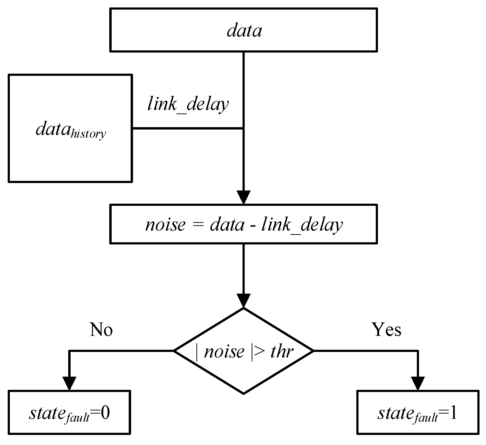
Due to the current lack of research on the integrity monitoring of time–frequency systems, the time–frequency signals output by the time–frequency signal generation and distribution subsystem in the time–frequency system use a very simple traditional monitoring algorithm. The principle and process are shown in Figure 10.
First, based on Equation (5), the link delay of each link is calculated by averaging the historical 30 min measurement data. Then, the noise of each link is calculated. The noise of each link is the corresponding link delay calculated in the first step deducted from the measurement data of each link. The noise of each link is near 0. Finally, the fault status is determined based on the fault threshold set by the user and the time difference measurement result. If the time difference measurement result exceeds the threshold, the link is considered to be faulty. On the contrary, if it is below the threshold, the link is considered to be trouble-free.
4.3.2. Experimental Scene and Parameter Setting
The scene of this experiment is consistent with the scene of the experiment described in Section 4.2.1 and will not be repeated here. And the threshold of this experiment is 500 ps, which is the index of the time–frequency system.
4.3.3. Experimental Results
For the scene of this experiment in Section 4.2.1, the traditional monitoring algorithm is used for integrity monitoring, and the status of the alarm and the TTA are shown in Table 5.
In Table 5, N/A means that the faults cannot be detected within 3 days after the faults occurs. It can be found that the traditional monitoring algorithm cannot accurately and effectively detect the small phase transition fault and the noise deterioration fault, and the detection effectiveness and real-time performance are weak. The detection ability of the traditional monitoring algorithm is closely related to the link itself, so its adaptability is weak. At the same time, for the frequency transition fault, the traditional monitoring algorithm takes 1 to 2 days to detect, and the real-time performance is weak.
In addition, by comparing the results of Table 4 and Table 5, it can be found that the integrity monitoring algorithm proposed in this paper has the following advantages compared with the traditional monitoring algorithm: the effectiveness and timeliness of fault detection are significantly improved, it can effectively detect multiple types of faults, and the real-time performance is increased by about 12 times. Therefore, the integrity monitoring algorithm proposed in this paper greatly improves the effectiveness, adaptability, and real-time performance of time–frequency signal monitoring.
In summary, the integrity monitoring algorithm proposed in this paper can effectively detect, identify, and alarm the phase transition fault, the noise deterioration fault, and the frequency transition fault. At the same time, the model proposed in this paper and the calculated integrity monitoring parameters have good adaptability. Compared with the traditional monitoring algorithm, the integrity monitoring algorithm proposed in this paper greatly improves the effectiveness, adaptability, and real-time performance of time–frequency signal integrity monitoring.
5. Conclusions
This paper focuses on the problem that the integrity monitoring of the time–frequency system is limited to the time–frequency signal output by the atomic clock group. By analyzing the theory of time–frequency source and link delay, it is found that temperature changes and frequency changes of the time–frequency signal are the main influencing factors of time difference measurement results. Therefore, a time–frequency signal integrity monitoring algorithm based on a temperature compensation frequency bias combination model is proposed. The algorithm analyzes the characteristics of time difference measurements, constructs a temperature compensation frequency bias combination model, and extracts and monitors the characteristics of the noise and frequency bias of the time difference measurement results, so as to realize the integrity monitoring of the time–frequency signal. The time difference measurement results of multiple links in a stably operating time–frequency system are used for verification. The conclusion is as follows:
- (1)
- Under the condition that the PFA is 10−3 and the PMD is 10−3, the typical value of the MDB is as follows: the phase transition is 86 ps, the STD of noise deterioration is 88 ps, and the frequency bias is 2 × 10⁻¹⁵.
- (2)
- Based on the typical value of the MDB and the calculated integrity monitoring parameters, the time difference measurement data of different links is used to construct a simulation experiment of the time–frequency signal fault of the corresponding link. The experimental results show that the algorithm in this paper can effectively detect, identify, and alarm the phase transition fault, the noise deterioration fault, and the frequency transition fault.
- (3)
- Additionally, the model and the integrity monitoring parameters developed in this paper exhibit high adaptability, making it directly applicable to the integrity monitoring of time–frequency signals across various links.
- (4)
- The traditional monitoring algorithm is used for fault simulation experiments, and the experimental results are compared with the experimental results of the algorithm in this paper. The experimental results show that the algorithm proposed in this paper greatly improves the effectiveness, adaptability, and real-time performance of time–frequency signal integrity monitoring.
Author Contributions
All authors contributed to the study conception and design. Y.G. designed and performed the experiments, analyzed the data, and wrote the paper. Z.L., H.G., J.P. and G.O. contributed to discussions and revisions. All authors have read and agreed to the published version of the manuscript.
Funding
This research was funded by the National Key R&D Program of China (grant number 2023YFC2205400), the National Natural Science Foundation of China (grant number U20A0193), and the Science and Technology Innovation Program of Hunan Province (grant number 2021RC3073).
Data Availability Statement
The datasets generated and/or analyzed during the current study are not publicly available due to the foundation requirements, but are available from the corresponding author on reasonable request.
Conflicts of Interest
The authors declare that the research was conducted in the absence of any commercial or financial relationships that could be construed as a potential conflicts of interest.
References
- Zheng, S.; Gao, M.; Huang, Z.; Jin, X.; Li, K. Satellite integrity monitoring for satellite-based augmentation system: An improved covariance-based method. Satell. Navig. 2022, 3, 9. [Google Scholar] [CrossRef]
- Wang, Y.; Shen, J. Real-time integrity monitoring for a wide area precise positioning system. Satell. Navig. 2020, 1, 24. [Google Scholar] [CrossRef]
- Chen, R.; Zhao, L. Multi-level autonomous integrity monitoring method for multi-source PNT resilient fusion navigation. Satell. Navig. 2023, 4, 21. [Google Scholar] [CrossRef]
- Zabalegui, P.; De Miguel, G.; Perez, A.; Mendizabal, J.; Goya, J.; Adin, I. A Review of the Evolution of the Integrity Methods Applied in GNSS. IEEE Access 2020, 8, 45813–45824. [Google Scholar] [CrossRef]
- Uwineza, J.-B.; Farrell, J.A. RAIM and Failure Mode Slope: Effects of Increased Number of Measurements and Number of Faults. Sensors 2023, 23, 4947. [Google Scholar] [CrossRef]
- Martin, A. RAIM Performance Analysis of Three Typical Low-Orbit Augmentation Constellations Combined with BDS Applications. Geomat. Inf. Sci. Wuhan Univ. 2023, 48, 678–686. [Google Scholar] [CrossRef]
- Liu, C.; Cao, Y.; Zhang, G.; Gao, W.; Chen, Y.; Lu, J.; Liu, C.; Zhao, H.; Li, F. Design and Performance Analysis of BDS-3 Integrity Concept. Remote Sens. 2021, 13, 2860. [Google Scholar] [CrossRef]
- Meng, Q.; Zhuang, Y.; Li, S. Implementation and Performance Analysis of Constellation Dynamic Selection in Multi-Constellation RAIM. Micromachines 2022, 13, 1455. [Google Scholar] [CrossRef]
- Blanch, J.; Walter, T. An Evaluation of the Advanced RAIM Threat Model. In Proceedings of the 2023 IEEE/ION Position Location and Navigation Symposium (PLANS), Monterey, CA, USA, 24–27 April 2023; pp. 408–413. [Google Scholar] [CrossRef]
- Chen, L.; Gao, W.; Hu, Z.; Cao, Y.; Pei, L.; Liu, C.; Zhou, W.; Liu, X.; Chen, L.; Yang, R. BDS-3 Integrity Risk Modeling and Probability Evaluation. Remote Sens. 2022, 14, 944. [Google Scholar] [CrossRef]
- Liu, J.; Zhao, X. GNSS Fault Detection and Exclusion Based on Virtual Pseudorange-Based Consistency Check Method. Chin. J. Electron. 2020, 29, 41–48. [Google Scholar] [CrossRef]
- Wang, H.; Cheng, Y.; Cheng, C.; Li, S.; Li, Z. Research on Satellite Selection Strategy for Receiver Autonomous Integrity Monitoring Applications. Remote Sens. 2021, 13, 1725. [Google Scholar] [CrossRef]
- Ma, X.; Yu, K.; He, X.; Li, Q.; Zhao, L.; Wang, H. Development and evaluation of a generalized model of RAIM availability for single-, dual- and multi-satellite faults. Meas. Sci. Technol. 2022, 33, 065022. [Google Scholar] [CrossRef]
- Sun, R.; Xu, C.; Huang, G.; Lan, X.; Wu, M. Multiple epochs solution separation RAIM algorithm considering alarm time. Syst. Eng. Electron. 2023, 45, 1469–1475. [Google Scholar] [CrossRef]
- Yu, Z.; Zhang, Q.; Zhang, S.; Zheng, N.; Liu, K. A state-domain robust autonomous integrity monitoring with an extrapolation method for single receiver positioning in the presence of slowly growing fault. Satell. Navig. 2023, 4, 20. [Google Scholar] [CrossRef]
- Sun, Y. RAIM-NET: A Deep Neural Network for Receiver Autonomous Integrity Monitoring. Remote Sens. 2020, 12, 1503. [Google Scholar] [CrossRef]
- Bhattacharyya, S. A computationally efficient Kalman filter-based RAIM algorithm for aircraft navigation with GPS and NavIC. Meas. Sci. Technol. 2023, 34, 125106. [Google Scholar] [CrossRef]
- Ren, Z.; Lyu, D.; Gong, H.; Peng, J.; Huang, X.; Sun, G. Continuous time and frequency transfer using robust GPS PPP integer ambiguity resolution method. GPS Solut. 2023, 27, 82. [Google Scholar] [CrossRef]
- Zhang, W.; Wang, J. Integrity monitoring scheme for single-epoch GNSS PPP-RTK positioning. Satell. Navig. 2023, 4, 10. [Google Scholar] [CrossRef]
- Wang, S.; Zhan, X.; Xiao, Y.; Zhai, Y. Integrity Monitoring of PPP-RTK Based on Multiple Hypothesis Solution Separation. In Proceedings of the 13th China Satellite Navigation Conference (CSNC)—Digital Economy and Intelligent Navigation, Beijing, China, 25–27 May 2022; pp. 321–331. [Google Scholar] [CrossRef]
- Zhang, W.; Wang, J.; El-Mowafy, A.; Rizos, C. Integrity monitoring scheme for undifferenced and uncombined multi-frequency multi-constellation PPP-RTK. GPS Solut. 2023, 27, 68. [Google Scholar] [CrossRef]
- Zhang, W.; Wang, J. GNSS PPP-RTK: Integrity monitoring method considering wrong ambiguity fixing. GPS Solut. 2024, 28, 30. [Google Scholar] [CrossRef]
- Gioia, C.; Borio, D. Multi-Layer Defences for Robust GNSS Timing Retrieval. Sensors 2021, 21, 7787. [Google Scholar] [CrossRef]
- Gioia, C.; Borio, D. Interference Mitigation and T-RAIM for Robust GNSS Timing; European Commission, Joint Research Centre: Ispra, Italy, 2021; pp. 70–79. [Google Scholar]
- Gioia, C. T-RAIM Approaches: Testing with Galileo Measurements. Sensors 2023, 23, 2283. [Google Scholar] [CrossRef]
- Tian, Y.; Wang, L.; Shu, B.; Han, Q.; Li, L.; Yi, C.; Xu, H. Evaluation of the availability of BDS ARAIM. Acta Geod. Cartogr. Sin. 2021, 50, 879–890. [Google Scholar]
- Cozzens, T. FAA Researching Advanced RAIM for GPS + Galileo Approaches. GPS World 2023, 34, 11. [Google Scholar]
- Patel, J.; Pervan, B. Accurate GPS LNAV parameters and clock biases for ARAIM offline monitoring. IEEE Trans. Aerosp. Electron. Syst. 2023, 59, 4313–4332. [Google Scholar] [CrossRef]
- Gao, W.; Yue, F.; Xu, Z.; Liu, P.; Li, D. Integrity Monitoring Methods of BDS Receiver Based on Inertial Assistance. Navig. Position Timing 2021, 8, 107–113. [Google Scholar] [CrossRef]
- Wu, K. Research on Autonomous Integrity Monitoring Technology of GNSS/INS Integrated Navigation Receiver. Master’s Thesis, National University of Defense Technology, Changsha, China, 2021. [Google Scholar]
- Xia, J.; Wang, S.; Jin, X.; Zeng, Q. Wi-Fi Assisted BDS Positioning Integrity Monitoring in Urban Cities. Geomat. Spat. Inf. Technol. 2022, 45, 15–17,23. [Google Scholar] [CrossRef]
- Zheng, H.; Atia, M.; Yanikomeroglu, H. Analysis of a HAPS-Aided GNSS in Urban Areas Using a RAIM Algorithm. IEEE Open J. Commun. Soc. 2023, 4, 226–238. [Google Scholar] [CrossRef]
- Jiang, H.; Li, T.; Song, D.; Shi, C. An Effective Integrity Monitoring Scheme for GNSS/INS/Vision Integration Based on Error State EKF Model. IEEE Sens. J. 2022, 22, 7063–7073. [Google Scholar] [CrossRef]
- Li, Y.; Xue, Y.; Chen, R.; Liu, Y. Research on Integrity Monitoring Method of Time-Frequency Signal. In Proceedings of the 3rd IEEE Advanced Information Technology, Electronic and Automation Control Conference (IAEAC), Chongqing, China, 12–14 October 2018. [Google Scholar]
- Wu, Y. Key Technologies of GNSS Time Scale. Ph.D. Thesis, National University of Defense Technology, Changsha, China, 2016. [Google Scholar]
- Wu, Y.; Zhu, X.; Huang, Y.; Sun, G.; Ou, G. Optimal Observation Intervals for Clock Prediction Based on the Mathematical Model Method. IEEE Trans. Instrum. Meas. 2016, 65, 132–143. [Google Scholar] [CrossRef]
- Li, X. Precision Measurement of Time and Frequency Signals; Science Press: Beijing, China, 2010; pp. 15–17. [Google Scholar]
- Baghdady, E.J.; Lincoln, R.N.; Nelin, B.D. Short-term frequency stability: Characterization, theory, and measurement. Proc. IEEE 1965, 53, 704–722. [Google Scholar] [CrossRef]
- Lesage, P.; Audoin, C. Characterization and measurement of time and frequency stability. Radio Sci. 1979, 14, 521–539. [Google Scholar] [CrossRef]
- Stein, S.R. Precision Frequency Control. In Frequency and Time-Their Measurement and Characterization; Gerber, E.A., Ballato, A., Eds.; Academic Press: New York, NY, USA, 1985; pp. 191–416. [Google Scholar]
- Li, Z. Time Frequency Measurement; Atomic Energy Press: Beijing, China, 2002; p. 296. [Google Scholar]
- William, R.; David, H. Handbook of Frequency Stability Analysis. Available online: https://tsapps.nist.gov/publication/get_pdf.cfm?pub_id=50505 (accessed on 22 December 2023).
- Dai, Q.; Yi, Q.; Yi, J. Research on Pulse Distribution Technology of High Precision. GNSS World China 2011, 6, 28–31. [Google Scholar] [CrossRef]
- Zhao, H.; Lv, Y.; Mei, P. A Digital High Precision Pulses Generation Method. Electron. Packag. 2017, 17, 23–25. [Google Scholar] [CrossRef]
- Zhong, W.; Gong, D.; Gong, H. A phase compensation method for time-frequency signal. J. Time Freq. 2011, 34, 16–22. [Google Scholar]
- Zhang, Y.; Yan, J. Compensation Method of Pressure Sensor Base on Minimum Two Multiplication Principle. Comput. Meas. Control 2007, 12, 1870–1871, 1874. [Google Scholar] [CrossRef]
- Zhu, J.; Cao, X.; Niu, Y.; Xiao, Z. Investigation of Lactone Chiral Enantiomers and Their Contribution to the Aroma of Longjing Tea by Odor Activity Value and S-Curve. J. Agric. Food Chem. 2023, 71, 6691–6698. [Google Scholar] [CrossRef]
- Kujawski, D.; Vasudevan, A.K.; Plano, S.; Gabellone, D. A method to estimate fatigue limit using (1/Nf)-S curve. Int. J. Fatigue 2024, 182, 108205. [Google Scholar] [CrossRef]
- Zhan, X.; Su, X. GNSS Integrity Monitoring Theory and Assisted Performance Enhancement Technique; Science Press: Beijing, China, 2016; p. 46. [Google Scholar]
Figure 1.
Architecture of a typical time–frequency system.

Figure 2.
Algorithm flowchart.

Figure 3.
Curve of time–frequency signal time difference measurement.

Figure 4.
Curve of ambient temperature change.

Figure 5.
The noise characteristics of the time–frequency signal time difference.

Figure 6.
Curve of the mean and RMSE of forecast bias.

Figure 7.
Curve of the PFA of various thresholds. (a) Curve of the PFA of the threshold of the mean of forecast bias; (b) Curve of the PFA of the threshold of RMSE; (c) Curve of the PFA of the threshold of frequency bias.
Figure 7.
Curve of the PFA of various thresholds. (a) Curve of the PFA of the threshold of the mean of forecast bias; (b) Curve of the PFA of the threshold of RMSE; (c) Curve of the PFA of the threshold of frequency bias.

Figure 8.
Curve of the PMD of various thresholds. (a) Curve of the PMD of the threshold of the mean of forecast bias; (b) Curve of the PMD of the threshold of RMSE; (c) Curve of the PMD of the threshold of frequency bias.
Figure 8.
Curve of the PMD of various thresholds. (a) Curve of the PMD of the threshold of the mean of forecast bias; (b) Curve of the PMD of the threshold of RMSE; (c) Curve of the PMD of the threshold of frequency bias.

Figure 9.
Simulation of time–frequency signal fault. (a) Simulation of phase transition fault; (b) Simulation of noise deterioration fault; (c) Simulation of frequency transition fault.
Figure 9.
Simulation of time–frequency signal fault. (a) Simulation of phase transition fault; (b) Simulation of noise deterioration fault; (c) Simulation of frequency transition fault.

Figure 10.
The process of the traditional monitoring algorithm.


Table 1.
The meaning of each parameter in process.
| Parameter | Meaning |
|---|---|
| dataold | Historical measurement data |
| ∆T | Historical temperature change data |
| data | Current measurement result |
| fb | Frequency bias |
| The STD of noise | |
| pdarr | Sequence of historical forecast bias |
| Threshold of RMSE | |
| thrpd | Threshold of forecast bias |
| Threshold of the mean of the forecast bias | |
| Mean of the historical forecast bias | |
| statematrix | Sequence of historical fault state |
| thrfb | Threshold of frequency bias |
| statefault | Fault Status at the current time |
| stateIntegrity | Integrity status at the current time |
Table 2.
Calculation results of model parameters.
| ftdata (Hour) | R | |||
|---|---|---|---|---|
| 1 | 0.53 | 8.96 × 10⁻¹⁵ | 0.34 | 18.40 |
| 2 | 0.14 | 4.74 × 10⁻¹⁵ | 0.38 | 10.06 |
| 3 | 0.29 | 4.42 × 10⁻¹⁵ | 0.27 | 9.19 |
| 4 | 0.31 | 4.58 × 10⁻¹⁵ | 0.21 | 9.38 |
| 5 | 0.35 | 4.07 × 10⁻¹⁵ | 0.16 | 8.30 |
| 6 | 0.47 | 2.35 × 10⁻¹⁵ | 0.15 | 4.85 |
| 7 | 0.70 | 1.30 × 10⁻¹⁵ | 0.13 | 2.74 |
| 8 | 0.67 | 1.20 × 10⁻¹⁵ | 0.12 | 2.61 |
| 9 | 0.69 | 8.55 × 10⁻¹⁶ | 0.14 | 2.13 |
| 10 | 0.81 | 3.85 × 10⁻¹⁶ | 0.07 | 1.14 |
| 11 | 0.87 | 3.13 × 10⁻¹⁶ | 0.09 | 1.30 |
| 12 | 0.91 | 2.36 × 10⁻¹⁶ | 0.05 | 1.80 |
| 13 | 1.01 | 1.30 × 10⁻¹⁶ | 0.06 | 2.40 |
| 14 | 1.01 | 8.94 × 10⁻¹⁷ | 0.04 | 2.80 |
| 15 | 1.01 | 8.87 × 10⁻¹⁷ | 0.03 | 2.94 |
| 16 | 0.93 | 9.36 × 10⁻¹⁷ | 0.02 | 2.96 |
| 17 | 0.92 | 9.81 × 10⁻¹⁷ | 0.04 | 2.98 |
| 18 | 0.92 | 8.06 × 10⁻¹⁷ | 0.02 | 2.99 |
| 19 | 0.90 | 5.96 × 10⁻¹⁷ | 0.04 | 3.00 |
| 20 | 0.95 | 1.97 × 10⁻¹⁶ | 0.08 | 3.00 |
| 21 | 1.01 | 2.46 × 10⁻¹⁶ | 0.07 | 3.12 |
| 22 | 1.06 | 2.85 × 10⁻¹⁶ | 0.04 | 3.56 |
| 23 | 1.07 | 2.93 × 10⁻¹⁶ | 0.04 | 3.69 |
| 24 | 1.06 | 2.98 × 10⁻¹⁶ | 0.02 | 3.55 |
Table 3.
Parameters of the experiment.
| Parameters | Meanings | Values |
|---|---|---|
| ftdata | The fitting time of data | 10 h |
| ATcon | The threshold of continuous fault alarm time | 5 s |
| thrpd | Threshold of the forecast bias | 3.1 |
| Tcp | Cumulative prediction time | 30 s |
| Threshold of the mean of the forecast bias | 50 ps | |
| Threshold for RMSE | 1.44 | |
| thrfb | Threshold for frequency bias | 1.5 × 10⁻¹⁵ |
Table 4.
Experimental results of parameter adaptability evaluation.
| Type of Faults | TTA(s) | ||||
|---|---|---|---|---|---|
| td1 | td2 | td3 | td4 | td5 | |
| Phase transition of 400 ps | 5 | 5 | 5 | 5 | 5 |
| Phase transition of 200 ps | 8 | 7 | 5 | 5 | 5 |
| Phase transition of 90 ps | 13 | 13 | 10 | 7 | 10 |
| Noise deterioration at 90 ps | 14 | 13 | 19 | 7 | 7 |
| Frequency transition of 2 × 10⁻¹⁵ | 7784 | 7666 | 7596 | 1846 | 7798 |
Table 5.
Experimental results of the traditional monitoring algorithm.
| Type of Faults | TTA(s) | ||||
|---|---|---|---|---|---|
| td1 | td2 | td3 | td4 | td5 | |
| Phase transition of 400 ps | 1463 | 1463 | 27788 | N/A | 10062 |
| Phase transition of 200 ps | N/A | N/A | N/A | N/A | N/A |
| Phase transition of 90 ps | N/A | N/A | N/A | N/A | N/A |
| Noise deterioration at 90 ps | 12,314 | 83,798 | 26,135 | N/A | N/A |
| Frequency transition of 2 × 10⁻¹⁵ | 89,666 | 107,408 | 135,189 | 182,726 | 160,450 |
Disclaimer/Publisher’s Note: The statements, opinions and data contained in all publications are solely those of the individual author(s) and contributor(s) and not of MDPI and/or the editor(s). MDPI and/or the editor(s) disclaim responsibility for any injury to people or property resulting from any ideas, methods, instructions or products referred to in the content. |
© 2024 by the authors. Licensee MDPI, Basel, Switzerland. This article is an open access article distributed under the terms and conditions of the Creative Commons Attribution (CC BY) license (https://creativecommons.org/licenses/by/4.0/).
Share and Cite
MDPI and ACS Style
Guo, Y.; Li, Z.; Gong, H.; Peng, J.; Ou, G. Time–Frequency Signal Integrity Monitoring Algorithm Based on Temperature Compensation Frequency Bias Combination Model. Remote Sens. 2024, 16, 1453. https://doi.org/10.3390/rs16081453
AMA Style
Guo Y, Li Z, Gong H, Peng J, Ou G. Time–Frequency Signal Integrity Monitoring Algorithm Based on Temperature Compensation Frequency Bias Combination Model. Remote Sensing. 2024; 16(8):1453. https://doi.org/10.3390/rs16081453
Chicago/Turabian StyleGuo, Yu, Zongnan Li, Hang Gong, Jing Peng, and Gang Ou. 2024. "Time–Frequency Signal Integrity Monitoring Algorithm Based on Temperature Compensation Frequency Bias Combination Model" Remote Sensing 16, no. 8: 1453. https://doi.org/10.3390/rs16081453
Note that from the first issue of 2016, this journal uses article numbers instead of page numbers. See further details here.