Locating and Grading of Lidar-Observed Aircraft Wake Vortex Based on Convolutional Neural Networks

Abstract

Aircraft wake vortices are serious threats to aviation safety. The Pulsed Coherent Doppler Lidar (PCDL) has been widely used in the observation of aircraft wake vortices due to its advantages of high spatial-temporal resolution and high precision. However, the post-processing algorithms require significant computing resources, which cannot achieve the real-time detection of a wake vortex (WV). This paper presents an improved Convolutional Neural Network (CNN) method for WV locating and grading based on PCDL data to avoid the influence of unstable ambient wind fields on the localization and classification results of WV. Typical WV cases are selected for analysis, and the WV locating and grading models are validated on different test sets. The consistency of the analytical algorithm and the CNN algorithm is verified. The results indicate that the improved CNN method achieves satisfactory recognition accuracy with higher efficiency and better robustness, especially in the case of strong turbulence, where the CNN method recognizes the wake vortex while the analytical method cannot. The improved CNN method is expected to be applied to optimize the current aircraft spacing criteria, which is promising in terms of aviation safety and economic benefit improvement.

1. Introduction

An aircraft wake vortex is a pair of vortex structures generated by the lift force exerted on aircraft wings, also called a “wing tip vortex”, which may cause serious damage to the following aircraft, especially during the landing and take-off phases [1,2]. Thus, most airports adopt regulations based on conservative separation for safety concerns, limiting airport capacity greatly. Facing the problems of safety and capacity, there have been a large number of studies on aircraft spacing and aircraft safety systems [3,4,5]. Theoretical research methods including numerical simulations and wind tunnel tests have been studied in depth to explore the characteristics of the evolutionary process of the wake vortex [6,7,8]. However, these methods can only simulate the wake vortex evolutionary process roughly due to the lack of high-precision atmospheric parameters, especially under near-surface conditions where the evolutionary characteristics of wake vortices are related to various factors such as headwind, crosswind, turbulence, etc.

In recent years, the Pulsed Coherent Doppler Lidar (PCDL) has become an effective method of aircraft wake vortex observation utilized by the International Civil Aviation Organization (ICAO) and has been employed across different platforms for the study of wake vortex characteristics and evolutionary processes under various circumstances [9,10,11,12,13]. The main characteristics of the wake vortex obtained via the PCDL are the wake vortex position and intensity, which are commonly utilized to track the evolutionary trajectory of the wake vortex and assess the potential hazards of the wake vortex intensity on the subsequent aircraft. Currently, the wake vortex retrieval algorithms based on PCDL data are mainly divided into two categories, the analytical algorithms and the machine learning algorithms.

The analytical algorithms of aircraft wake vortex recognition mainly focus on how to calculate the position of wake vortices and the circulation value representing the intensity of wake vortices precisely in previous literature. The commonly used methods primarily include the velocity envelope method and the radial velocity method, both of which calculate the characteristic parameters of wake vortices such as core position, tilt angle, circulation, and so on based on the velocity fields obtained via PCDL measurements. The velocity envelope method can obtain precise vortex parameters based on tangential velocity, which requires relatively high signal-to-noise ratio (SNR) lidar data [9]. The radial velocity method was proposed for the estimation of wake vortex parameters under stationary conditions and weak turbulence, giving an equivalent error on core position and a larger relative error of 20% on circulation estimation, compared to the velocity envelope method [12]. The specific impact of the circulation error on aircraft spacing during take-off and landing phases needs to be evaluated based on parameters such as the circulation value, background wind field condition, turbulence intensity, and other relevant factors. The two methods can be combined to achieve higher positioning accuracy to solve the incorrect location caused by complex background wind fields and strong turbulence, with a faster speed [13,14]. The correction method of circulation estimation is used to avoid the underestimation and overestimation of vortex circulation, caused by the relative movement between the laser beam and the wake vortex under near-ground effect [2].

The analytical algorithm plays a vital role in the analysis of the wake vortex evolutionary process. However, it cannot meet the requirement of obtaining wake vortex parameters in real time for air traffic control due to the limitation of computing resources. In recent years, deep learning methods have been used widely, to provide a new method for fast analysis of characteristics of aircraft wake vortices. The deep learning algorithms primarily ascertain the presence of wake vortices and identify their respective spatial regions utilizing image feature recognition. The existence of wake vortex has been studied by employing various deep learning models based on image data sets, achieving good accuracy [15,16,17]. The deep learning models also showed their applicability in the estimation of wake vortex parameters including the vortex core position and vortex intensity [18,19]. The image data sets used in the above existing algorithms are solely derived from the radial wind velocities, which require a relatively stable ambient wind field, resulting in insufficient anti-interference ability. In radial velocity images, the structure of the wake vortex is susceptible to influences from turbulence, gusts, and other factors. Meanwhile, the resulting variations in image features caused by wind speed fluctuations are potentially recognized as a wake vortex. That is, there will be misidentification and missing identification when strong turbulence or interference exists. A deep learning method based on frequency-domain data obtained from PCDLs is presented to reduce the effect of disturbances by combining both radial velocity and spectrum width, achieving good accuracy on wake vortex recognition.

This paper is composed of five sections. Section 2 introduces the methods to construct the data sets and to train the deep learning models for wake vortex locating and grading. Section 3 provides the models’ performance including typical cases and statistical evaluation. Section 4 discusses the reason for the different performances of the models considering the climatological information. Section 5 summarizes the conclusion and outlook of this paper.

2. Methodology

2.1. Experiments and Data

The evolution of a wake vortex is closely related to terrain, climate, and weather conditions. The observation experiments were conducted at two different airports located in East China and Southwest China, respectively, to explore the characteristic difference of the wake vortex caused by meteorological and topographic factors.

The locations of Chengdu Shuangliu International Airport (ZUUU) and Qingdao Liuting International Airport (ZSQD) are shown in Figure 1a. The former is a subtropical monsoon climate with high temperature and humidity in summer, located in the basin. The latter is a temperate monsoon climate, with high wind speed in spring, located in the coastal hills. The number of effectively observed aircraft sorties exceeded 4000 (totally observed sorties > 8000), with the lidar configured at ZUUU from August 2018 to September 2018 and at ZSQD from November 2019 to June 2020, respectively. The PCDL at ZUUU was configured southeast of Runway 02, about 1400 m vertically from the landing point, aiming to observe landing aircraft, as shown in Figure 1b,d. The PCDL at ZSQD was configured southeast of Runway 35, about 400 m away from the observation positions, to observe aircraft in the take-off phase, as shown in Figure 1c,e.

The PCDL system employed during the experiments was Wind3D 6000, manufactured by Leice Transient Technology Co., Ltd., achieving high-precision wind field measurement [20,21]. The PCDLs employed Range-Height-Indicator (RHI) scanning mode for wake vortex observation. The resolution of the PCDL elevation angle was set to be 0.2 degrees per second at ZUUU and 0.4 degrees per second at ZSQD to ensure a consistent vertical resolution of the wake vortex data, considering the relative position of the PCDLs. During the experiments, the range resolution of the PCDLs was set to 15 m, providing sufficient vertical resolution for observing wake vortices. The parameters of the PCDL scanning strategy during the experiments at ZUUU and ZSQD are listed in

Table 1. Parameters of the PCDL scanning strategy during the experiments at ZUUU and ZSQD.

Parameters	ZUUU	ZSQD
	Landing	Take-Off
Scanning mode	RHI	RHI
Scanning speed	~1°/s	~2°/s
Azimuth angle	90°	260°
Elevation angle range	0~10°	2~35°
Elevation angle resolution	0.2°	0.4°
Scanning duration	~10 s	~17 s

. The elevation angle range of PCDL at ZSQD was larger than that at ZUUU, since the flight path of the aircraft during take-off is more uncertain than the flight path of the aircraft during landing and the former PCDL was much closer to the landing point. Considering the vertical resolution, the elevation angle resolution of the PCDL at ZUUU was much lower than that at ZSQD.

The data source used in this paper were frequency-domain data (simply called FD data in this paper), which can be obtained via transforming time-domain data—the processed backscattered signal obtained using PCDLs and the Fast Fourier Transform (FFT) method [20]. FD data are the fundamental data for wind field retrieval obtained using a Doppler lidar, providing atmospheric information including radial velocity, turbulence characteristics, and the signal-to-noise ratio [2,22]. The data sets used for the wake vortex locating and grading modules were established separately based on FD data, namely the radial velocity (RV)-spectrum width (SW) data set and the wake vortex (WV) region data set. The RV-SW data sets are composed of the radial velocity and spectrum width data obtained at all observing elevations and ranges, while the WV region data set contains only limited elevations and ranges where the wake vortex exists.

The data sets of the wake vortex were established not only based on the wake vortex characteristics from PCDL data but also adjusted considering flight information. A dynamic matching algorithm including two matching processes was proposed in our previous work [23]. Two matching processes were used to select effective wake vortex observation data for different flights and the identification of the start and end times of the wake vortices. Firstly, matching between the PCDL scanning times and the flight take-off and landing times was performed. Then, the start and end times of the current flight’s wake vortices were obtained via the second match, which was used for the establishment of wake vortex data sets. The process of adjusting the wake vortex data sets using flight information is considered as empirical correction in this paper.

Three RV-SW data sets and one WV region data set were established by matching the PCDL data with flight information. The former data sets were used to compare the different models’ performance on different test sets, to explore the different characteristics of wake vortices under different meteorological and topographical conditions. The latter data set was used to verify the feasibility of the wake vortex grading method, composed of lidar data at ZUUU. The composition of the data sets is shown in

Table 2. Composition of the wake vortex locating and grading data sets.

Data Sets	Corresponding Model	Airport/No.
RV-SW data set 1	WV locating model	ZUUU/1000
RV-SW data set 2	WV locating model	ZSQD/1000
RV-SW data set 3	WV locating model	ZUUU/1000 + ZSQD/1000
WV region data set	WV grading model	ZUUU/2000

. In all the data sets, the ratio of the training set to the test set was 8:2.

2.2. Wake Vortex Retrieval Algorithms

The analytical algorithm and the deep learning algorithm are the two approaches used to obtain the position and intensity information of the wake vortex. In this paper, the results retrieved from the analytical algorithm were used as the reference while establishing data sets to train the deep learning models. In our previous study, it was found that the analytical algorithm could not recognize the wake vortex where interference exists, such as an undissipated wake vortex or strong turbulence. Thus, the parameters of wake vortex characteristics were adjusted empirically according to flight information and vortex temporal evolutionary characteristics, due to the lack of infallible truth of the wake vortex.

The algorithm of aircraft wake vortex locating and grading consists of four parts—data pre-processing, WV locating, WV grading, and model evaluation—as shown in Figure 2. A detailed description of all the parts will be provided in the following sections.

2.2.1. Data Pre-Processing

The step of data pre-processing aims to provide a reliable data set for model training. In this section, a new wake vortex image data set named the RV-SW data set is put forward and tested for training the deep learning models, using the radial velocity and spectrum width images obtained from the analytical algorithm. The process of data pre-processing and analysis of images is explained below.

The radial velocity and spectrum width can be retrieved using the analytical algorithm, according to the three velocities retrieved from FD data by using a given threshold [13]. The radial velocity contains the peak value of FD data, and the spectrum width contains the broadening information due to turbulence. The existence of the wake vortex affects the nearby local wind field, generating a Doppler broadening phenomenon of a spectrum width, as well as the wind pair structure in radial velocity, which can be clearly seen in the pseudo-color images at a distance of about 320 m and a height of about 120 m, as shown in Figure 3a,b. The features in radial velocity and spectrum width can be used for wake vortex identification by employing deep learning methods.

Disturbances such as the presence of noise and errors will greatly affect the accuracy of wake vortex identification when using radial velocity or spectrum width separately [24]. For example, the wake vortex structure will be interfered with by the strong turbulence and could not be well displayed in RV images, while it is obvious in the SW images. In contrast, the RV image can better highlight the existence of the wake vortex when its circulation is relatively small and the background wind field is relatively stable, whereas the SW image is less obvious or even disappears in this case, which is related to the selection of the threshold value.

Thus, the RV-SW data set is used in this paper, to incorporate as much information as possible. The radial velocity image and spectrum width image are converted to gray-scale and stacked to obtain the RV-SW data set, aiming to combine the wind pair features in radial velocity with the broadening features in spectrum width. The gray-scale images of radial velocity and spectrum width are shown in Figure 3c,d, with the grays-cale range from 0 to 255, where the brighter color represents a larger value. The stacked image is shown in Figure 3e, where the ratio of radial velocity to spectrum width was 1:2.

2.2.2. Wake Vortex Locating

The position of the vortex core is necessary information for analyzing the evolutionary trajectory of the wake vortex. Turbulence and other disturbances always affect the accuracy of localization since the analytical algorithm recognizes horizontal features and vertical features separately. The deep learning model is used to identify the overall characteristics of the wake vortex to improve its anti-interference ability, which is illustrated in this section. Firstly, the wake vortex position is retrieved using analytical algorithms with empirical correction. Then, the WV locating model is trained. Finally, the wake vortex region without background disturbances is extracted.

The analytical method combines both radial velocity and spectrum width data for wake vortex localization, as described in our previous research [2,13]. The horizontal position of the vortex core is retrieved according to the distribution of the maximum and minimum radial velocity and the maximum value of the spectrum width at each range bin. The vertical position of the vortex core is obtained from the middle position of the maximum and minimum velocity envelope. Empirical correction according to flight information and vortex evolutionary characteristics is added since there would be missing recognition and misrecognition results when using the analytical algorithm. The wake vortices can be marked as the regions shown in the white dashed boxes in Figure 4.

As a one-stage object detection algorithm with high precision, the You Only Look Once (YOLO) network has become the most frequently used object detection deep learning model [25]. The YOLO models can recognize the location of all the objects labeled as different classes and provide the most-possible regions with their possibilities. In this paper, the YOLO v4 model integrating the characteristics of the former versions is chosen for wake vortex localization.

YOLO v4 consists of three parts: CSP Darknet53 is the main backbone, Spatial Pyramid Pooling (SPP) and Path Aggregation Network (PAN) are the neck network, and the YOLO head is the prediction structure. The CSPNet enables rich gradient combinations with less computational effort and higher accuracy, reducing computational bottlenecks and costs and enhancing learning ability [26]. The SPP is utilized as a solution for the problem of fixed-size constraints when dealing with the images [27]. The PAN is employed to boost the flow of information, achieving better feature fusion [28]. The head of YOLO v4 obtains the results of recognition using the obtained features, the same as the head of YOLO v3 [29]. The model mainly employs the CIoU (Complete-Intersection over Union) loss as the bounding box location loss [30], of which the confidence loss and classification loss are the same as YOLO v3. The structure of the WV locating model is shown in Figure 5.

The parameters for the training of the WV locating model based on RV-SW data set 3 (mentioned in Table 2) are shown in

Table 3. Parameters of deep learning model for wake vortex locating based on RV-SW images.

Parameter	Value
Input size	416 × 416
Classes	1
Learning rate	1 × 10−4
Batch size	4
Iterations	6400

. Only the wake vortex structure is labeled with the coordinates of its region to remove the influence of background turbulence for subsequent intensity grading, so the number of classes is only 1. Thus, the WV locating model could provide the coordinates of a rectangular region that is most likely to be the wake vortex class with its possibility. The learning rate is set to be 1 × 10⁻⁴ and the batch size is chosen to be 4, corresponding to 6400 iterations.

The coordinates of the wake vortex would be obtained by employing the trained and validated WV locating model. Then, the features of the wake vortex are extracted to reduce the effect of disturbances in the ambient wind field, which cause inaccurate results of wake vortex identification according to our earlier work using analytical methods. The extracted wake vortex regions are shown in Figure 6.

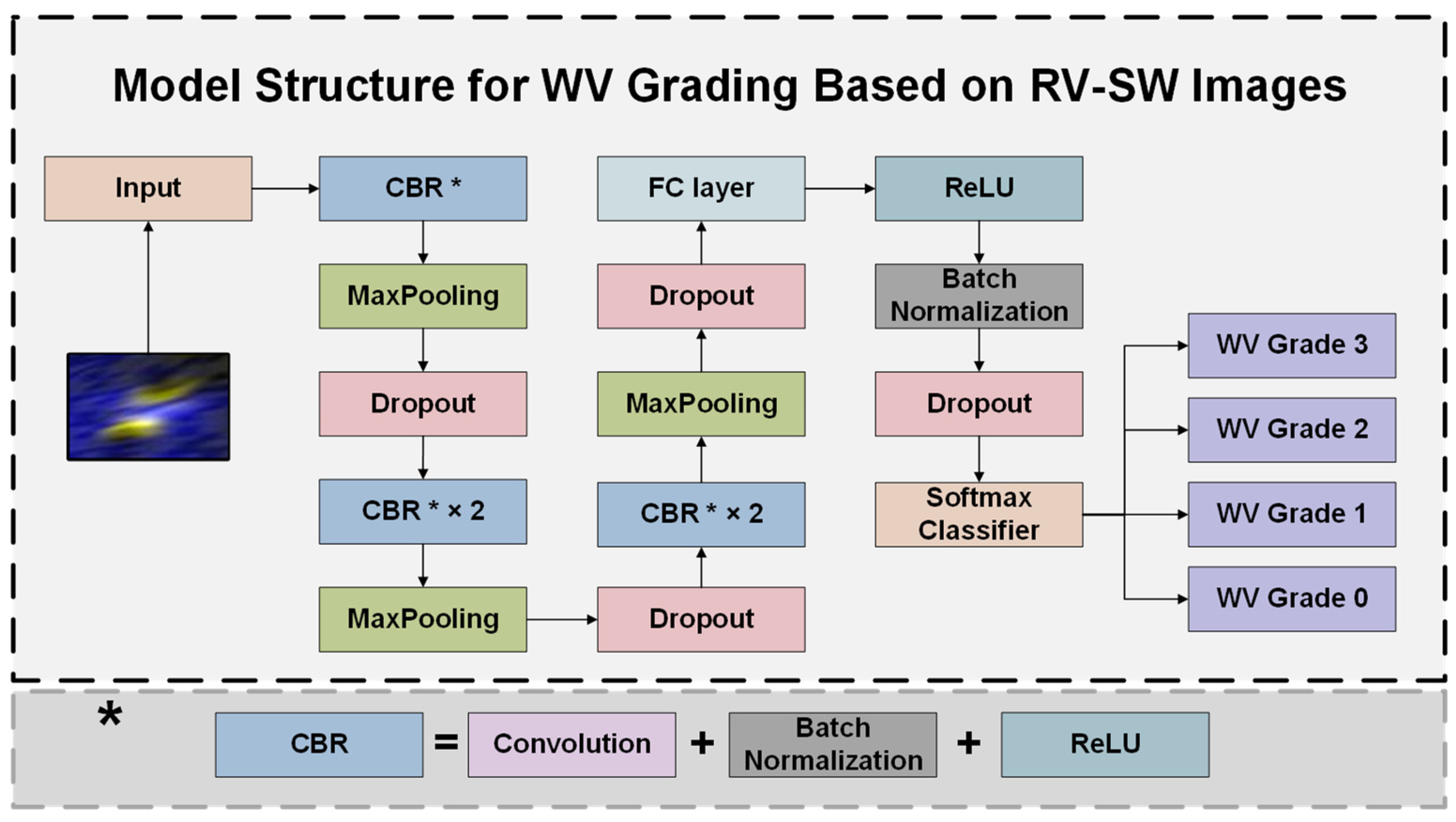
2.2.3. Wake Vortex Grading

The circulation value is another key parameter to evaluate the risk of the wake vortex, representing vortex intensity. The biggest error source of wake vortex intensity estimation is inaccurate positioning due to the disturbances. Thus, the feature classification model is employed to obtain the intensity grades of the wake vortex regions, which are provided according to the results of wake vortex localization. The deep learning method proposed in this section can effectively reduce the evaluation error and avoid the influence of interference compared to traditional algorithms. The data set observed at ZUUU is selected for the feasibility evaluation of the WV grading model. Firstly, the wake vortex circulation is retrieved using analytical algorithms with empirical correction. Then, the WV grading model is trained.

The analytical algorithms calculate the wake vortex circulation according to the distribution of tangential velocity based on the assumption that the vortex structure is circular and axisymmetric [31]. The velocity envelope is required to calculate the vortex circulation, which represents the sum of the tangential velocity and the background radial velocity, assuming that the distance between the vortex core and the sensing volume is short enough [9]. Meanwhile, the scaling correction was performed to avoid the stretching and compression caused by the relative movement of the wake vortex and the laser beam [2]. Then, the WV region data set is divided into four grades according to data characteristics, through the comparison of the models’ performances based on different settings. Empirical correction according to flight information and vortex evolutionary characteristics is also conducted. For example, the misidentification of disturbance will be eliminated and the missing wake vortex will be added, referring to the circulation values of the previous and the latter wake vortex. The grading standard of the WV region data set is shown in

Table 4. Grading standard of WV region data set for deep learning model training.

Intensity Grade	Circulation Value	Number of WV
Grade 3	More than 600	500
Grade 2	350~600	500
Grade 1	100~350	500
Grade 0	Less than 100 or disturbances	500

.

The Visual Geometry Group (VGG) network was proposed for the improvement of the model’s accuracy by increasing its depth steadily by only using very small convolution filters [32]. In VGG networks, the 3 × 3 convolution filters are stacked to achieve the same effective receptive field of larger filters, and the 2 × 2 max-pooling layers are used after each convolutional layer to reduce the computation of the model. A more compact VGG network structure is used for wake vortex classification to reduce feature parameters and save computing costs, which could significantly increase the ability to obtain image features and improve the model’s performance. Only one fully connected layer with the ReLU activation function is applied differently from the three connected layers in classic VGG networks. The model structure for WV grading is shown in Figure 7.

Parameters of the deep learning model for wake vortex grading based on the ZUUU WV region data set can be seen in

Table 5. Parameters of deep learning model for wake vortex grading based on WV region images.

Parameter	Value
Input size	96 × 96
Classes	4
Learning rate	5 × 10−4
Batch size	8
Iterations	4800

. The learning rate is set to be 5 × 10⁻⁴, after comparing different orders of magnitude of learning rates, to avoid the oscillation of validation loss. The batch size is adjusted to be 8, thus the number of iterations is 4800. Note that the convergence of the grading model is closely related to the selection of data sets and the setting of network parameters. The model may fail to converge if the feature distinction between different grades is not obvious or the batch size is too large.

2.2.4. Evaluation Metrics

The performance of the models should be evaluated comprehensively after obtaining the WV locating and grading models for continuous optimization and improvement. Precision, Recall, F1-score, mean Average Precision (mAP), and Kappa coefficient are the parameters commonly used for model evaluation.

The formulas of Precision and Recall are shown as Equation (1) and (2). True Positive (TP), False Positive (FP), and False Negative (FN) are introduced, to calculate the value of Precision and Recall. Precision is defined as the number of positive samples predicted to be positive (TP) divided by the total number of samples predicted to be positive (TP + FP), representing the prediction accuracy in the samples that are predicted to be positive. Correspondingly, Recall measures the ratio of positive samples predicted to be positive (TP) out of all positive samples (TP + FN), representing the prediction accuracy in positive samples.

$$Precision=\frac{TP}{TP+FP}$$

(1)

$$Recall=\frac{TP}{TP+FN}$$

(2)

F1-score gives equal weight to Precision and Recall, which is used as a common index in the evaluation of model performance. The formula of F1-score is explained as Equation (3).

$$F1=2\times \frac{Precision\times Recall}{Precision+Recall},$$

(3)

In addition, mAP is also a vital parameter that evaluates the performance of the models. The formulas of AP and mAP are shown as Equations (4) and (5). Where $ri$ is the Recall value at the position of the point $i$ after interpolation of the Precision-Recall (P-R) curve, and $Pinter$ is the Precision value after interpolation, obtained according to the value of the maximum Precision on the right side of all the chosen points. Thus, AP measures the ability of the trained model to detect the category of interest, while mAP represents the ability of the trained model to detect all categories. The parameter $k$ is the number of categories.

$$AP={\displaystyle \sum _{i=1}^{n-1}(ri+1-ri)Pinter(ri+1)} , mAP=\frac{{\displaystyle {\sum }_{i=1}^{k}APi}}{k}$$

(4)

$$Pinter(r)=\max r^{\prime }\ge rP(r^{\prime })$$

(5)

Kappa coefficient is another index used for consistency tests, measuring the accuracy of classification. Kappa coefficient can be calculated according to the result of the confusion matrix, shown in Equation (6). Here, $po$ is the ratio of the sum of the diagonal elements in the confusion matrix to the sum of the entire matrix elements, $pe$ is the ratio of the sum of the product of actual and predicted quantities corresponding to all categories, respectively, to the square of the total number of samples.

$$Kappa=\frac{po-pe}{1-pe}$$

(6)

3. Results

3.1. Measurement Cases

The accuracy and effectiveness of the CNN algorithm can be verified through comparison with results from analytical algorithms with flight information. The applicability of the two methods under different conditions is demonstrated, including the wake vortex under the stable meteorological condition and the wake vortex under the strong turbulence condition, by conducting extensive processing and comparative analysis. In this section, two representative measurement cases are presented to illustrate the performance of the CNN algorithm.

3.1.1. Wake Vortex under Stable Meteorological Condition

A typical case of a well-structured wake vortex observed at 12:42, 25 August 2018, at ZUUU is shown in Figure 8, which can be effectively recognized by both two algorithms. The value of turbulence—Energy Dissipation Rate (EDR)—is used to evaluate the turbulence in this paper [2]. The EDR^1/3 of the vortex-free PCDL data in the adjacent moment at the height of 20 m to 60 m is calculated to be 0.09 m^2/3 s⁻¹, much less than the ICAO standard. Thus, the ambient wind field is considered to be relatively stable.

The spectrum width and radial velocity of the well-structured wake vortex are shown in Figure 8a,b, the wake vortex core positions obtained from the analytical algorithm are (491.6 m, 36.8 m) and (521.5 m, 39.1 m), representing the horizontal and vertical distance from the lidar, respectively. The circulation values of the left and right vortex are 221.5 m² s⁻¹ and 149.2 m² s⁻¹, respectively, summed to be 370.7 m² s⁻¹.

The results of CNN algorithms are shown in Figure 8c. The result recognized by the WV locating model is [224, 152, 284, 197], representing the coordinates of left x, upper y, right x, and lower y of the wake vortex region in the image, respectively. The WV region extracted based on the coordinates above is classified into Grade 2 via the WV grading model, consistent with the analytical algorithm, referring to the criteria in Table 4. The CNN algorithm and the analytical algorithm show good consistency within this presented case, with high possibilities of 0.99 on locating and 88.41% on grading.

3.1.2. Wake Vortex under Strong Turbulence Condition

Another typical case of a wake vortex under the turbulence condition, observed at 12:14, 27 August 2018, at ZUUU, is shown in Figure 9. The EDR^1/3 of the vortex-free data in the adjacent moment at the height of 10 m to 50 m is calculated to be 0.31 m^2/3 s⁻¹, much larger than that in Case 1, considered as moderate turbulence according to the ICAO standard (regarded as the strong turbulence condition in this paper).

The images of spectrum width and radial velocity of the wake vortex under strong turbulence condition are shown in Figure 9a,b, the former is hardly affected by turbulence, while the instability of the background wind field can be seen in the latter image. The horizontal location of the wake vortex obtained by the analytical algorithm is shown in Figure 9c. The horizontal positions of the vortex cores can be marked by two peaks in $SR\_ind$, considering both $SW\_ind$ and $RV\_ind$ [2,13]. It can be seen that there is only one single peak on the black line due to the influence of turbulence, so the analytical algorithm could not obtain the position of the wake vortex nor could it calculate the circulation value.

The CNN algorithm could recognize the whole feature of the wake vortex in the RV-SW image, rather than the feature of a single dimension as the analytical algorithm does, which can avoid the interference of turbulence. The result of the WV locating model is [216, 172, 271, 215] with the possibility of 0.84, and the result of the WV grading model is Grade 2 with the possibility of 86.82%, less than that in Case 1, as shown in Figure 9d. The decrease in certainty also proves that the model has higher accuracy when the wake vortex is well-structured with a stable background wind field.

These two representative cases provide a visual demonstration of the CNN algorithm’s performance for the locating and grading of a wake vortex under stable and strong turbulence conditions. In these cases, the CNN algorithm and the analytical algorithm show a good agreement when the background wind field is stable, and the former method could recognize wake vortices when the effectiveness of the latter method is greatly affected under strong turbulence conditions. Meanwhile, it is also explained that the accuracy of the CNN algorithm will be influenced by atmospheric turbulence to some extent.

3.2. Statistical Evaluation

The performances and robustness of deep learning models can be evaluated statistically based on different test sets by calculating the parameters explained in Section 2.2.4. The test results of four WV locating models trained on different training data sets are compared, and the effectiveness of the WV grading model is also assessed. The parameters are calculated according to Equations (1)–(6), where the F1-score, mAP, and Kappa coefficient can evaluate the performance of the models more thoroughly by comprehensively considering the Precision and Recall rate.

3.2.1. Performance of WV Locating Model

Based on historical weather data, the experiments at ZUUU were primarily conducted during the summer, with predominantly overcast and rainy conditions and less frequent sunny and cloudy days, of which the temperatures were generally above 20 degrees Celsius. The ZSQD experimental data were mostly obtained during the spring, characterized by predominantly clear and cloudy skies, with frequent rainfall and temperatures ranging from as low as 5 degrees to as high as 20 degrees Celsius. Additionally, ambient wind speeds were often light during observations at ZUUU, which were typically between force 2–4, with variable wind directions at ZSQD. By selecting typical data from clear, cloudy, and rainy days for calculation, it was found that the mean value of EDR^1/3 at different altitudes at ZUUU did not exceed 0.15 m^2/3 s⁻¹, which was over 0.15 m^2/3 s⁻¹ for one-third of the time at ZSQD, with a larger overall fluctuation range, indicating more variable turbulence characteristics. Overall, the meteorological environment during the experiment at ZUUU was more stable, whereas the background wind field and climatic conditions were more diverse during the experiment at ZSQD.

Four models based on different data sets were trained and tested to evaluate the model’s performance under the different conditions of the two airports, as

Table 6. Performance of WV locating models based on different training sets and test sets.

Model	Training and Validation Set	Test Set (Airport/No.)	Precision	Recall	F1	mAP
1	RV-SW data set 1(ZUUU)	ZUUU/200	99.5%	94.1%	0.97	99.4%
		ZSQD/200	97.8%	43.8%	0.60	82.8%
2	RV-SW data set 2 (ZSQD)	ZUUU/200	92.0%	84.7%	0.88	89.7%
		ZSQD/200	96.2%	87.1%	0.91	96.7%
3	ZUUU model + ZSQD data set	ZUUU/200	99.5%	94.1%	0.97	99.4%
		ZSQD/200	93.6%	57.7%	0.71	89.4%
4	RV-SW data set 3 (ZUUU + ZSQD)	ZUUU/200	99.0%	97.5%	0.98	99.9%
		ZSQD/200	98.3%	87.6%	0.93	98.6%

shows. WV locating model 1 and 2 were trained using the RV-SW data set observed at ZUUU and ZSQD, respectively. Both WV locating model 3 and 4 employed ZUUU and ZSQD data, the difference is that the former was trained by adding the ZSQD data set to the ZUUU model, and the latter was trained using ZUUU and ZSQD data sets simultaneously. The WV locating models have certain differences between the test sets, due to the diversity in the background wind field, experimental durations, and other factors in the training and validation data sets.

• The WV locating model performs well when the training set and the test set are built based on the same data set. The F1-score and mAP of model 1 are 0.97 and 99.4% when applied to the ZUUU test set and 0.60 and 82.8% when applied to the ZSQD test set. It can be seen that model 1 has good performance on the ZUUU test set but does not perform well on the ZSQD test set. The Precision value of 97.8% means that most of the wake vortices identified using the CNN algorithm are consistent with the reference values in the data set, but the Recall value of 43.8% shows that more than half of the wake vortex cannot be identified.
• A new model can be obtained by adding data from a specified airport to build a new training set or continually training based on a current model, showing better performance at the specified airport. Model 3 was trained on the ZSQD data set based on model 1, and the Precision value decreases while the Recall value increases when applying to the ZSQD test set, meaning that the missing wake vortex images of the model are reduced, at the cost of a slight increase in the misidentification rate.
• The model trained on a mixed data set performs better on each test set compared to the model continually trained on the added data based on a current model. Although both model 3 and model 4 were trained based on all data of the two airports, model 4 trained on RV-SW data set 3 performed better with F1-scores of 0.98 and 0.93 and mAPs of 99.9% and 98.6% when applied on the ZUUU test set and ZSQD test set, respectively.
• Models trained on more diverse data sets have higher generalization ability. As mentioned above, the observation environment at ZSQD was more complicated than that at ZUUU, which means the data set established at the former airport is more diverse than the data set formed based on the latter. The F1-score and mAP of model 2 applied on the ZUUU test set are 0.88 and 89.7%, higher than the test results of model 1 applied on the ZSQD test set, for which the parameters are 0.60 and 82.8%.

3.2.2. Performance of WV Grading Model

The confusion matrix is used to evaluate the feasibility of the WV grading model, as shown in Figure 10. Where the horizontal axis represents the predicted results and the vertical axis represents the true results. The model performs better in Grades 0 and 2, the reason for which may be that the wake vortex features of Grades 0 and 2 are more unique. The former has more chaotic image features, and the latter has a clearer wake vortex structure. The features of the wake vortex of Grade 1 and 3 are not clear enough due to the high wind speed or the dissipating wake vortex.

Precision, Recall, and F1-score can also be calculated to evaluate the performance of the WV grading model based on the confusion matrix, as shown in

Table 7. Performance of WV grading model based on different training sets and test sets.

Model	Data Set	Grade	Precision	Recall	F1
WV grading model	WV region data set (ZUUU)	0	99.0%	98.0%	0.98
		1	97.9%	95.0%	0.96
		2	98.0%	100.0%	0.99
		3	97.0%	96.0%	0.96

. The macro average values of Precision, Recall, and F1-score are calculated to be 98.0%, 97.3%, and 0.97, respectively. In addition, the Kappa coefficient of the WV grading model is 0.97 (much larger than 0.8—the threshold for determining the model’s performance), showing that the predicted results are in good agreement with the wake vortex reference values.

In this section, the CNN algorithm is proved to have good consistency with the analytical algorithm. The migration application ability and robustness of the WV locating model on different test sets are compared. The WV grading model is also proved to be feasible. It has been validated that the analytical algorithm takes approximately one minute to retrieve the wake vortex location and circulation, with empirical corrections added to ensure accuracy. In contrast, the deep learning method completes the entire process in about 15 s, significantly improving the efficiency of wake vortex recognition and providing a quasi-real-time approach for wake vortex parameters.

4. Discussion

In Section 3.2.1, this paper compares the performance of the CNN algorithm in identifying wake vortices based on the data observed at two airports, as shown in Table 6. For instance, models trained on the ZSQD data set outperform those trained on the ZUUU data set, and models considering all data from both airports exhibit higher accuracy than those trained exclusively on a single airport data set. Meteorological environmental factors during the PCDL observation experiments at the two airports may be one of the primary reasons for these results.

We selected typical historical meteorological data for clear, cloudy, and rainy days to compute the EDR^1/3 during the observation periods at ZUUU and ZSQD, as illustrated in Figure 11. The results for ZUUU are indicated by round dots, while the results for ZSQD are indicated by diamond dots. Specifically, the results for 27 August, 5 September, and 7 September 2018 correspond to clear, rainy, and cloudy days, respectively, from Shuangliu District, Chengdu City, while those for 6 April, 12 April, and 8 May 2020 correspond to cloudy, clear, and rainy days, respectively, from Chengyang District, Qingdao City. Among the selected historical data, Chengdu exhibited higher temperatures ranging from 18 to 33 degrees Celsius, with background wind conditions being calm or light breezes; Qingdao had lower temperatures between 4 and 17 degrees Celsius, with background wind fields consisting of southeast wind at a force of two, northwest wind at a force of three, and east wind at a force of three.

The average results of the EDR^1/3 within the 5–80 m near-ground layer for typical date data from the two airports are shown in Figure 11. The missing data indicate periods when the lidar was not operational during the night or when data were rendered unusable due to rainfall interference. It can be deduced that the ZUUU data exhibit lower EDR values, below 0.15 m^2/3 s⁻¹, whereas the ZSQD data show a broader fluctuation range between 0 and 0.2 m^2/3 s⁻¹. The EDR^1/3 for all three days decreases around 5:00–6:00, with greater relative fluctuations on rainy days at ZUUU; the EDR for all three days drops around 15:00, with clear and cloudy days showing larger fluctuations at different times, while the EDR on rainy days maintains a relatively stable high value at ZSQD.

Given the climatic differences between the two aforementioned airports and the disparities in calculated EDR values, further elucidation of the varying test accuracies of the models can be attempted. The model trained on the ZUUU data set has predominantly learned wake vortex characteristics under more stable environments, hence its subpar performance on the ZSQD test set. Conversely, the model trained on the ZSQD data set has learned more diverse features, giving better identification accuracy across both test sets. Similarly, supplementing the model trained on the ZUUU data set with additional ZSQD data, which encompasses a wider range of wake vortex evolutionary characteristics, enhances its precision when applied to the ZSQD test set, and vice versa. The model trained on both data sets from ZUUU and ZSQD has acquired the most varied features, leading to commendable performances on the test sets from both airports.

From Figure 11, we could conclude that wake vortex models are influenced by the background environmental conditions present in their training data sets. Models trained on data sets with more homogeneous features also possess some recognition capabilities for data with more diverse features, though they tend to have a higher rate of False Negatives. Therefore, when employing the CNN algorithm for wake vortex recognition, incorporating as many characteristic wake vortex data as possible into the training set may enhance the model’s applicability across different airport data sets.

5. Conclusions

This paper presents a deep learning method for aircraft wake vortex localization and classification based on Pulsed Coherent Doppler Lidar data observed at ZUUU and ZSQD. The method consists of using the WV locating and WV grading modules to avoid the influence of unstable ambient wind fields. Data sets are built based on the analytical algorithm with empirical correction according to flight information and the evolutionary characteristic of the wake vortex. Several models are trained and evaluated based on different data sets. The CNN algorithm is proved to have good consistency and better robustness compared with the analytical algorithm, based on the measurement cases and statistical evaluation methods. The deep learning method has broad application prospects in the field of aviation safety, with the ability to provide a quasi-real-time reference value for the analysis of aircraft wake vortices.

The major conclusions are summarized as follows:

• A deep learning method for wake vortex locating and grading is presented based on stacked radial velocity and spectrum width images, obtained from FD raw data. Three data sets are built under different meteorological and topographical conditions (ZUUU and ZSQD airports) and used for the training and testing of four WV locating models, to evaluate model performances under different conditions. The WV grading model is trained and tested based on the ZUUU data set, to verify the effectiveness of the model.
• The WV locating models are trained based on different data sets, showing certain differences in the test sets. The performance of the models can be summarized as follows: The WV locating model performs well when the training set and the test set are built based on the same data set. A new model can be obtained by adding data from a specified airport to build a new training set or continually training based on a current model, showing better performance at the specified airport. The model trained on a mixed data set performs better on each test set compared to the model continually trained on the added data based on a current model. Models trained on more diverse data sets have higher generalization ability.
• The WV grading model is verified to be effective for the classification of WV region images. The removal of the non-WV region could amplify wake vortex features, to improve the accuracy of the model. According to the confusion matrix and statistical evaluation parameters, the predicted results are in good agreement with the wake vortex reference values, based on the analytical algorithm and empirical correction.
• The deep learning method in this paper has good performance not only when applied to the well-structured wake vortex but also to wake vortices under strong turbulence conditions, where the analytical algorithm cannot recognize the structure of the wake vortex. The deep learning algorithm and the analytical algorithm have been verified for consistency. The former exhibits better robustness and a faster processing speed of approximately 15 s.

This paper has provided an attempt at wake vortex locating and grading using an improved deep learning method. In the future, the data sets could be further expanded for training and testing, and the performance of the model trained using various data sets can be compared. The time variable can be considered to further improve the accuracy of the model. The models can be used to identify and analyze the characteristics of wake vortices under various meteorological conditions, to further optimize the spacing criteria of airports.

References

1. Breitsamter, C. Wake vortex characteristics of transport aircraft. Prog. Aerosp. Sci. 2011, 47, 89–134. [Google Scholar] [CrossRef]
2. Wu, S.; Zhai, X.; Liu, B. Aircraft wake vortex and turbulence measurement under near-ground effect using coherent Doppler lidar. Opt. Express 2019, 27, 1142–1163. [Google Scholar] [CrossRef] [PubMed]
3. Gerz, T.; Holzäpfel, F.; Bryant, W.; Köpp, F.; Frech, M.; Tafferner, A.; Winckelmans, G. Research towards a wake-vortex advisory system for optimal aircraft spacing. C. R. Phys. 2005, 6, 501–523. [Google Scholar] [CrossRef]
4. Hinton, D.A. A Candidate Wake Vortex Intensity Definition for Application to the NASA Aircraft Vortex Spacing System (AVOSS); National Aeronautics and Space Administration, Langley Research Center: Washington, DC, USA, 1997; Volume 110343, pp. 4–25. [Google Scholar]
5. Perry, R.; Hinton, D.; Stuever, R.; Perry, R.; Hinton, D.; Stuever, R. NASA wake vortex research for aircraft spacing. In Proceedings of the 35th Aerospace Sciences Meeting and Exhibit, Hampton, VA, USA, 6–9 January 1997. [Google Scholar] [CrossRef]
6. Hallock, J.N.; Holzäpfel, F. A review of recent wake vortex research for increasing airport capacity. Prog. Aerosp. Sci. 2018, 98, 27–36. [Google Scholar] [CrossRef]
7. Hennemann, I.; Holzäpfel, F. Large-eddy simulation of aircraft wake vortex deformation and topology. Proc. Inst. Mech. Eng. 2011, 225, 1336–1350. [Google Scholar] [CrossRef]
8. Brandon, J.M.; Jordan, F.L., Jr.; Stuever, R.A.; Buttrill, C.W. Application of Wind Tunnel Free-Flight Technique for Wake Vortex Encounters; No. NAS 1.60: 3672; NASA Center for AeroSpace Information: Linthicum Heights, MD, USA, 1997. [Google Scholar]
9. Köpp, F.; Rahm, S.; Smalikho, I. Characterization of aircraft wake vortices by 2-μm pulsed Doppler lidar. J. Atmos. Ocean Technol. 2004, 21, 194–206. [Google Scholar] [CrossRef]
10. Rahm, S.; Smalikho, I. Aircraft wake vortex measurement with airborne coherent Doppler lidar. J. Aircr. 2008, 45, 1148–1155. [Google Scholar] [CrossRef]
11. Smalikho, I.N. Taking into account the ground effect on aircraft wake vortices when estimating their circulation from lidar measurements. Atmos. Ocean. Opt. 2019, 32, 686–700. [Google Scholar] [CrossRef]
12. Smalikho, I.N.; Banakh, V.A.; Holzäpfel, F.; Rahm, S. Method of radial velocities for the estimation of aircraft wake vortex parameters from data measured by coherent Doppler lidar. Opt. Express 2015, 23, A1194–A1207. [Google Scholar] [CrossRef] [PubMed]
13. Hallermeyer, A.; Dolfi-Bouteyre, A.; Valla, M.; Brusquet, L.L.; Fleury, G.; Thobois, L.P.; Cariou, J.-P.; Duponcheel, M.; Winckelmans, G. Development and assessment of a Wake Vortex characterization algorithm based on a hybrid LIDAR signal processing. In Proceedings of the 8th AIAA Atmospheric and Space Environments Conference, Washington, DC, USA, 13–17 June 2016. [Google Scholar] [CrossRef]
14. Liu, X.; Zhang, X.; Zhai, X.; Zhang, H.; Liu, B.; Wu, S. Observation of aircraft wake vortex evolution under crosswind conditions by pulsed coherent Doppler lidar. Atmosphere 2020, 12, 49. [Google Scholar] [CrossRef]
15. Pan, W.; Duan, Y.; Zhang, Q.; Tang, J.; Zhou, J. Deep learning for aircraft wake vortex identification. In IOP Conference Series: Materials Science and Engineering; IOP Publishing: Bristol, UK, 2019. [Google Scholar] [CrossRef]
16. Pan, W.; Yi, H.; Leng, Y.; Zhang, X. Recognition of aircraft wake vortex based on random forest. IEEE Access 2022, 10, 8916–8923. [Google Scholar] [CrossRef]
17. Pan, W.; Wu, Z.; Zhang, X. Identification of aircraft wake vortex based on SVM. Math. Probl. Eng. 2020, 2020, 9314164. [Google Scholar] [CrossRef]
18. Duan, Y.; Yi, W. Research on aircraft wake vortex recognition based on YOLO artificial intelligence. J. Ordnance Equip. Eng. 2020, 41, 242–247. [Google Scholar]
19. Wartha, N.; Stephan, A.; Holzäpfel, F.; Rotshteyn, G. Characterizing aircraft wake vortex position and intensity using LiDAR measurements processed with artificial neural networks. Opt. Express 2022, 30, 13197–13225. [Google Scholar] [CrossRef] [PubMed]
20. Wu, S.; Liu, B.; Liu, J.; Zhai, X.; Feng, C.; Wang, G.; Zhang, H.; Yin, J.; Wang, X.; Li, R.; et al. Wind turbine wake visualization and characteristics analysis by Doppler lidar. Opt. Express 2016, 24, A762–A780. [Google Scholar] [CrossRef]
21. Zhang, H.; Wu, S.; Wang, Q.; Liu, B.; Yin, B.; Zhai, X. Airport low-level wind shear lidar observation at Beijing Capital International Airport. Infrared Phys. Technol. 2019, 96, 113–122. [Google Scholar] [CrossRef]
22. Yuan, J.; Xia, H.; Wei, T.; Wang, L.; Yue, B.; Wu, Y. Identifying cloud, precipitation, windshear, and turbulence by deep analysis of the power spectrum of coherent Doppler wind lidar. Opt. Express 2020, 28, 37406–37418. [Google Scholar] [CrossRef] [PubMed]
23. Wang, X.; Wu, S.; Liu, X.; Yin, J.; Pan, W.; Wang, X. Observation of aircraft wake vortex based on coherent Doppler lidar. Acta Opt. Sin. 2021, 41, 901001–901018. [Google Scholar]
24. Gao, H.; Li, J.; Chan, P.W.; Hon, K.K.; Wang, X. Parameter-retrieval of dry-air wake vortices with a scanning Doppler Lidar. Opt. Express 2018, 26, 16377–16392. [Google Scholar] [CrossRef] [PubMed]
25. Sultana, F.; Sufian, A.; Dutta, P. A review of object detection models based on convolutional neural network. Intell. Comput. Image Process. Based Appl. 2020, 1157, 1–16. [Google Scholar] [CrossRef]
26. Wang, C.Y.; Liao, H.Y.M.; Wu, Y.H.; Chen, P.Y.; Hsieh, J.W.; Yeh, I.H. CSPNet: A new backbone that can enhance learning capability of CNN. In Proceedings of the IEEE/CVF Conference on Computer Vision and Pattern Recognition Workshops, Seattle, WA, USA, 13–19 June 2020. [Google Scholar] [CrossRef]
27. He, K.; Zhang, X.; Ren, S.; Sun, J. Spatial pyramid pooling in deep convolutional networks for visual recognition. IEEE Trans. Pattern Anal. Mach. Intell. 2015, 37, 1904–1916. [Google Scholar] [CrossRef] [PubMed]
28. Liu, S.; Qi, L.; Qin, H.; Shi, J.; Jia, J. Path aggregation network for instance segmentation. In Proceedings of the IEEE Conference on Computer Vision and Pattern Recognition, Salt Lake City, UT, USA, 18–23 June 2018. [Google Scholar] [CrossRef]
29. Redmon, J.; Farhadi, A. Yolov3: An incremental improvement. arXiv 2018, arXiv:1804.02767. [Google Scholar]
30. Zheng, Z.; Wang, P.; Liu, W.; Li, J.; Ye, R.; Ren, D. Distance-IoU loss: Faster and better learning for bounding box regression. In Proceedings of the AAAI Conference on Artificial Intelligence, New York, NY, USA, 7–12 February 2020. [Google Scholar] [CrossRef]
31. Holzäpfel, F.; Gerz, T.; Köp, F.; Stumpf, E.; Harri, M.; Youn, R.I.; Dolfi-Bouteyre, A. Strategies for circulation evaluation of aircraft wake vortices measured by lidar. J. Atmos. Ocean. Technol. 2003, 20, 1183–1195. [Google Scholar] [CrossRef]
32. Simonyan, K.; Zisserman, A. Very deep convolutional networks for large-scale image recognition. In Proceedings of the 3rd International Conference on Learning Representations, San Diego, CA, USA, 7–9 May 2015. [Google Scholar] [CrossRef]
Figure 1. Information of experiments for wake vortex observation based on PCDL. (a) Location of ZUUU and ZSQD. (b) Sketch map of wake vortex observation experiments at ZUUU. (c) Sketch map of wake vortex observation experiments at ZSQD. (d) Lidar position and scanning mode of wake vortex observation experiments at ZUUU. (e) Lidar position and scanning mode of wake vortex observation experiments at ZSQD.
Remotesensing 16 01463 g001
Figure 2. Flow chart of the main methodology of aircraft wake vortex locating and grading algorithm.
Remotesensing 16 01463 g002
Figure 3. Images of wake vortex observed at ZSQD at 00:47 on 27 April 2020, LST, where the brighter color represents a larger value. (a) The pseudo-color images of radial velocity (RV). (b) The pseudo-color images of spectrum width (SW); (c) The gray-scale images of RV. (d) The gray-scale images of SW. (e) The stacked image of radial velocity and spectrum width (RV-SW).
Remotesensing 16 01463 g003
Figure 4. RV-SW images after marking the regions of the wake vortices with dashed boxes, where the brighter color represents a larger value. (a,b) RV-SW images with marked wake vortex regions at ZSQD. (c,d) RV-SW images with marked wake vortex regions at ZUUU.
Remotesensing 16 01463 g004
Figure 5. The structure of the WV locating model based on YOLO v4 with different color blocks representing different layers. The color blocks marked with * are the results of combining different layers, the structure of which are explained in the lower part of the diagram marked with *.
Remotesensing 16 01463 g005
Figure 6. The WV region data set after extracting the wake vortex feature from the RV-SW data set, where the brighter color represents a larger value. (a) Example of Grade 0. (b) Example of Grade 1. (c) Example of Grade 2. (d) Example of Grade 3.
Remotesensing 16 01463 g006
Figure 7. The structure of the deep learning model used for wake vortex grading based on WV region images with different color blocks representing different layers. The color blocks marked with * are the results of combining different layers, the structure of which are explained in the lower part of the diagram marked with *.
Remotesensing 16 01463 g007
Figure 8. The images and results of the wake vortex under stable meteorological condition. (a) Spectrum width image of the wake vortex. (b) Radial velocity image of the wake vortex. (c) Results of WV locating and grading models when applied on the wake vortex, where the brighter color represents a larger value.
Remotesensing 16 01463 g008
Figure 9. The images and results of the wake vortex under strong turbulence condition. (a) Spectrum width image of the wake vortex. (b) Radial velocity image of the wake vortex. (c) Results of horizontal location of the wake vortex when using the analytical algorithm, where the light blue line represents S W _ i n d , the light pink line represents R V _ i n d , and the black line represents S R _ i n d , the red pentagram represents the location of the vortex core as identified by the algorithm. (d) Results of WV locating and grading models when applied on the wake vortex, where the brighter color represents a larger value.
Remotesensing 16 01463 g009
Figure 10. The confusion matrix of the WV grading model.
Remotesensing 16 01463 g010
Figure 11. The value of EDR1/3 of typical dates at ZUUU and ZSQD.
Remotesensing 16 01463 g011