
Short-Term Foredune Dynamics in Response to Invasive Vegetation Control Actions


Faculdade de Ciências, Instituto Dom Luiz, Universidade de Lisboa, 1749-016 Lisboa, Portugal
*
Author to whom correspondence should be addressed.
Remote Sens. 2024, 16(9), 1487; https://doi.org/10.3390/rs16091487
Submission received: 27 February 2024
/
Revised: 13 April 2024
/
Accepted: 17 April 2024
/
Published: 23 April 2024
(This article belongs to the Special Issue Remote Sensing Application in Coastal Geomorphology and Processes II)
Abstract
:Efforts to control the spread of invasive alien species (IAS) in coastal dunes are essential to protect biodiversity and maintain the integrity of the ecosystem. However, the timing and extent of these control measures often do not consider their potential impact on dune morphodynamics. This study investigated how IAS control measures can affect sand dune mobility. Research involved monitoring short-term morphological and vegetation changes using close-range remote sensing along with historical wind data. Findings revealed that changes in vegetation cover significantly impacted dune system evolution, notably increasing sand mobility when IAS vegetation was removed. Considering the seasonal wind regime, dominated by offshore winds in the summer, removing vegetation during this period can promote seaward sediment transport, potentially resulting in sediment loss to the beach. These findings highlight the importance of understanding sediment mobility patterns when planning vegetation control actions within dune restoration strategies.
1. Introduction
Coastal foredunes are wind-blown sand accumulations that develop on the backshore by aeolian sand deposition within vegetation [1,2]. They correspond to shore-parallel convex ridges [1] and constitute effective obstacles regarding wave overtopping and coastal flooding. Moreover, sediment stored in foredunes is readily transferred to the beach during storms and is naturally returned to the dune in favorable conditions. This morphological flexibility increases resilience of the coastal zone to coastal hazards and risks. As a natural coastal defense, dunes are currently considered as fundamental elements to be preserved, also integrating a range of adaptation measures to mitigate adverse effects of climate change [3,4,5,6,7].
Beach–dune systems provide attractive landscapes for tourism activities and are under intense pressure due to coastal development. Increasing human occupation near the coastline has caused the fragmentation and degradation of these ecosystems [8,9]. In terms of vegetation, this degradation is also often associated with the introduction and spread of invasive alien species (IAS) as a means of stabilizing/retaining dune sands [10,11].
Due to the significant ecological importance of coastal dunes, they are subject to frequent restoration initiatives that typically entail the eradication of IAS and, in some cases, the reintroduction of native flora [4,12]. In addition, there are different goals for coastal dune restoration, including stabilizing dunes by increasing vegetation cover or, conversely, reactivating stabilized dunes by removing vegetation. The latter increases aeolian dynamics and facilitates landward sand transport, with the aim of increasing habitat diversity [9,13,14]. However, some authors [15] question the restoration value of this type of intervention, arguing that dune sealing by vegetation, accompanied by reduced mobility, may represent the natural evolutionary path of this type of coastal system, as observed by [16].
Dune restoration involving vegetation replacement is a two-step process in which the removal of the undesirable (usually invasive) vegetation precedes seeding or planting of the replacement (usually native) vegetation. The introduction of replacement (native) vegetation faces several constraints, such as mortality, that contribute to the time lag between vegetation removal and re-covering of the sandy surface. During this time, vegetation cover is low and the exposed sandy area is more vulnerable to wind. According to [13,17,18] this can lead to an increase in sand mobility, resulting in geomorphic changes.
While it is recognized that removing plants suddenly can increase sand mobility, the optimal spatial range and timing for this removal has been inadequately explored, especially concerning the directional patterns of effective wind and potential sand transport during restoration.
The aim of this research is to investigate how the extent and timing of dune vegetation control measures impact foredune sand mobility. This is especially relevant in contexts where the wind regime exhibits strong seasonal variations, which affect the onshore vs. offshore aeolian sand transport and have implications for the overall dune sand budget. This study focuses on a semi-stabilized foredune system with limited sand supply that is exposed to seasonal contrasting winds. Foredune sand mobility patterns were assessed using close-range remote sensing, alongside hindcast wind data. During the monitoring period, the system was subject to several IAS control measures. The data for this study were collected as part of the EU LIFE Dunas project (LIFE 19 CCA/PT/001178).
2. Study Area
The area addressed herein is located on the southwest tip of Porto Santo island, a volcanic island part of the Madeira Archipelago (Portugal), in the North Atlantic Ocean. The island is surrounded by a set of islets (Figure 1) and shows a NE-SW elongated shape, with an area of about 42 km2. The island has an extensive embayed beach–dune system (9 km) located on the south coast [19], which is protected from the prevailing northerly waves by the island shadow effect.
Porto Santo’s climate is semi-arid according to the Köppen–Geiger climate classification [20]. Rainfall is very reduced (annual average of about 400 mm) with the rainy season (October to March) concentrating 80% of the annual precipitation. The mean annual temperature is 18 °C with a small thermal amplitude over the year [19,21,22,23]. There are no permanent rivers; the drainage network is composed of gullies and temporary streams.
Regarding the wind regime (direction and average speed), the dominant winds in Porto Santo blow from northern sectors (64%) with the north octant representing about 37% of the occurrences [21,22]. Winds from the SE direction are the lowest in frequency and calms represent 5% of occurrences. The average wind speed is about 5.6 m/s. Both authors above based their analysis on the 1961–1990 records from the only existing meteorological station on the island (Porto Santo/Aeroporto) located in the airport.
In the study area (which extends over about 50 × 103 m2) and surroundings, a number of geomorphological units were identified (Figure 1) as described below. Porto Santo beach is intermediate-reflective with a limited sand supply and is limited landward by a foredune, that reaches about 12 m above the mean sea level (a.s.l.). A second dune ridge is present, separated from the foredune by a dune slack (or interdune area). In its central region, the foredune ridge has retreated and merged with the second dune [21], configuring a curved plane shape. This has allowed for the development of an aeolian deflation basin, the onset of which has been linked to sand exploitation in the 20th century [19,23].
Further inland, the dune connects to a gently sloping seaward surface defined by colluvial deposits [21], where agricultural practices developed until the mid-20th century; since then, agriculture has been abandoned and aeolian sand has advanced over agricultural land. On the seaward side, the foredune articulates with the beach directly or through discontinuous rocky outcrops of aeolianite (wind-blown calcareous Pleistocene sandstones), locally covered by a thin layer of sand and patches of dark basalt pebbles. Further seaward, the beach limits with a low intertidal rocky platform were developed in aeolianite and beach rock (not defined in Figure 1), which is occasionally exposed at low tide. This stretch of coastline is oriented at about 50°–230° relative to true North.
Beach and dune sediments are of medium sand size and essentially composed of organogenic carbonate sands (calcareous algae and bivalve shell remains, among others) resulting from the erosion of the aeolianites, with the addition of minor contributions of shells of present-day marine organisms; in addition, fragments of rock and minerals from the erosion of volcanic rocks also occur [21,23].
Dune vegetation is essentially composed of herbaceous species [24,25] with an average height ranging from 0.2 m to 1 m. As of October 2020, herein taken as the reference situation, the vegetation cover was around 30% on the leeward slope and 15% on the windward slope, as determined from orthomosaics derived from high-resolution aerial photographs (see Section 3.4. Image Classification and Vegetation Changes). Species spatial zoning is not evident, although some shrubs (e.g., Tamarix gallica) and fig trees are observed, mainly near the dune crest and on its leeward side.
T. gallica, together with Arundo donax, was introduced in the agricultural area near the landward dune toe to delimit the private land parcels and prevent incoming windblown sand. T. gallica, A. donax and Carpobrotus edulis are invasive species [26] and they have spread out over the dune and adjacent agricultural parcels because of the abandonment of agriculture, inhibiting the development of autochthonous species. A. donax and C. edulis were targeted for eradication, whereas T. gallica was subjected to pruning. In October 2020 and according to the vegetation inventory of November 2020 [27], A. donax was by far the most abundant invasive species, largely outnumbering both C. edulis and T. gallica and usually covering more than 50% of the sampled areas. Other exotic, albeit non-invasive species have been catalogued and covered less than 5% of the sampled areas.
Among the native species present in the study area are Calystegia soldanella, Polygonum maritimum, Euphorbia paralias, Lotus glaucus and Lotus lowenus (the latter being endemic to Porto Santo) [28,29].
C. edulis was eradicated by manual uprooting (hand-pulling) during 2021, and by April 2022 it had been almost eliminated from the intervened area [27]. Control of A. donax began in the summer of 2021 using brushcutters. However, this method was later replaced by mechanical uprooting by the end of the same year. Chemical treatment was also introduced in May 2022. Due to rhizome sprouting, multiple interventions were necessary in both the NE and SW dune sections.
Vegetation control measures translated to a reduction of approximately one-third of the total vegetation cover from early 2021 to the end of 2022 [27]. This change was primarily due to the fall in coverage of A. donax to less than half of its initial coverage (Figure 2). Native species were only planted experimentally in November 2021 and April and November 2022, in small plots located in the western and eastern dune sections. The total area involved was very small (approximately 600 m2) and therefore did not significantly affect the overall vegetation cover.
3. Materials and Methods
3.1. UAV Surveys
Unmanned aerial vehicles (UAVs) provide an effective and reliable means of monitoring changes in coastal environments (e.g., [7,30,31,32,33,34,35,36]), which can often be subjected to rapid morphological changes. UAV-derived products also allow for the synchronous assessment of land cover (e.g., [7,36]).
Six aerial UAV surveys were conducted between October 2020 and February 2023 using a DJI Drone model MAVIC 2 PRO (Model L1 S/N163DF9300100UB) equipped with a 20-megapixel Hasselblad RGB camera. Surveys were performed in automatic flight mode configured using the Pix4Dcapture application. The flight altitude ranged from 60 m a.s.l. in October 2020 to 50 m a.s.l. for the other five surveys (Supplementary Materials, Table S1). The flight path of each survey was defined to provide 90% front overlap and 70% side overlap between images. Sets of ground control points (GCPs) were distributed on the dune and adjacent beach before each survey (Supplementary Materials, Figure S2, Table S1) and measured with RTK-GPS equipment (Leica Viva CS10 NetRover S/N2521082). RTK-GPS measurements were carried out at an accuracy better than 0.05 m with real-time differential correction provided by the REPGRAM (Rede Regional de Estações Permanentes da Região Autónoma da Madeira) service.
Similarly to [37,38], the images obtained from each UAV survey were used in the Structure from Motion process with AgiSoft Metashape Profissional photogrammetric software (Version 1.7.3. build 12473-64bit). This allowed for the reconstruction of a three-dimensional model, from which an RGB orthomosaic and a digital surface model (DSM) were generated. Both output products used the PTRA08 UTM Zone 28N coordinate system. The pixel resolution of the output orthomosaics was 0.015 m, while the resolution of the DSM was 0.025 m, with the exception of the October 2020 survey, which was processed at 0.030 m (Supplementary Materials, Table S1). For data standardization, the latter DSM was resampled to match the resolution of every other DSM (0.025 m).
Validation of DSM accuracy was conducted by estimating the root mean square error (RMSE) between modeled surfaces and the GCP positions surveyed in the field using RTK-GPS. It is worth noting that these GCPs were the same ones used for generating the surface model. The horizontal and vertical errors were assessed using the horizontal (XY) and vertical (Z) displacements between datasets and include the entire surveyed area. These metrics were calculated using AgiSoft’s standard error report options. Furthermore, an independent evaluation of each DSM of the study area was performed by comparing elevation data from control profiles (PPS1 to PPS4—see Figure 1) that were surveyed using RTK-GPS, during each field campaign, with homologous points in the DSM. The module of elevation deviations, RMSE and bias were calculated.
3.2. Wind Data
Wind data for the study area were extracted from the ECMWF’s ERA5 atmospheric reanalysis of the global climate [39], hereafter referred to as the ERA5. The atmospheric parameters extracted consist of the u-component (eastward) and v-component (northward) of the wind velocity 10 m above the sea surface at an hourly base. The selected grid point (16.25°W; 33.00°N) is located offshore of Porto Santo beach (Figure 1) and is part of a global grid with a spatial resolution of 0.25°.
Wind regime characterization was performed by statistical analysis over a period of 24 years between January 1999 and February 2023. To assess its representativeness, we compared wind speed and direction data from the Porto Santo Airport, the only meteorological station on the island, with ERA5 data from 2000 to 2020.
For comparison between the wind regime and morphological variations observed during the study period, a shorter data-series was extracted covering a time span of three years, between 12 April 2020 and 25 February 2023. These data are presented in five sets, that include the wind analyzed between field campaigns and the wind analyzed for a 6-month period before the first field campaign.
Aeolian sand transport is initiated when the wind shear stress on grains populating the surface exceeds a critical value, termed the “static threshold”. However, once sand movement begins, its maintenance requires a lower stress value, referred to as the “dynamic threshold” [40,41].
Both the static and the dynamic thresholds were estimated following the Bagnold formulation [40] (Equation (1)). The critical wind speeds at 10 m corresponding to both thresholds were estimated according to [40], Equation (2) (which was based on Prandtl and von Karman’s formulation of the logarithmic wind profile), replacing with and with .
where —shear velocity threshold (m/s); —dimensionless coefficient: 0.1 for start of movement and 0.08 for transport maintenance; —particle specific mass (2768 kg/m3 in the study area); —air specific mass (1.225 kg/m3); —acceleration of gravity (9.81 m/s2); and —mean grain diameter (0.00027 m in the study area).
where —wind velocity (m/s), at distance above the ground; —wind shear velocity (m/s), replaced by (determined as 0.245 m/s, taking = 0.1, and determined as 0.196 m/s, taking = 0.08); —height above ground of wind measurement (10 m); —height of focal point, determined as 0.005 m for the study area; and —wind velocity at (determined as 3.860 m/s, taking = 0.1, and determined as 3.088 m/s, taking = 0.08). These parameters yielded wind speeds at 10 m () of 8.5 m/s for the static threshold and of 6.8 m/s for the dynamic threshold (threshold conditions indicated by the subscript t).
3.3. Potential Aeolian Transport
Potential wind transport between campaigns was calculated to investigate the effect of wind seasonality on the potential transfer of sand from the beach to the dune, which implied considering only winds with an onshore velocity component. The Bagnold formula [40], which states that the rate of aeolian transport is proportional to the cube of wind shear velocity (Equation (3)), was used for this purpose.
where is the potential sand transport rate in kg/(m.s); is a dimensionless empirical constant that takes the following values: 1.5 for very well-sorted sand, 1.8 for well-sorted sand, and 2.8 for poorly sorted sand; herein, we considered = 1.8 in agreement with textural data; and is the diameter of standard particles (0.00025 m).
The results were expressed in volumetric units (m3) by dividing the transport rate by the specific mass of bulk dry sediment and correspond to the shore-normal total potential transport between successive campaigns. Values were also octant-estimated and normalized to the number of days (month).
3.4. Image Classification and Vegetation Changes
Vegetation cover and changes were identified in classified orthomosaics generated through an unsupervised automatic classification process. The iso cluster classifier was employed for this procedure, resulting in orthomosaics featuring two classes: bare sand and vegetation. The vegetation class represents all dark features in the images of the area, including vegetation, its shadows, and several dark pebbles distributed mainly in the deflation basin and on the beach. Temporal mapping of the IAS control actions on different sectors of the study area was achieved by comparing successive classified images. This information, evaluated in conjunction with volume changes, enabled the determination of the specific locations and time periods in which IAS controls affected different sectors of the foredune.
3.5. Morphological Changes and Sediment Budget
To investigate morphological changes between surveys, the DSMs were compared using elevation difference maps and trend analysis. Morphological variations of less than 0.10 m in elevation were considered not significant. The trend analysis was performed over a DSM multidimensional raster dataset, generated with the DSM previously produced, considering a linear fit of elevation (pixel variable) through time. A positive slope corresponds to a trend of increase in height and a negative slope corresponds to a decrease.
Calculation of the sediment budget relied upon the elevation difference maps. The latter were converted to volumetric difference maps by multiplying each pixel value by the pixel area. The sediment budget was then obtained by summing the pixel values (volume) considering each geomorphological unit. The limits between different units were mapped considering the orthomosaics and DSM produced by the October 2020 UAV survey and field photographs. Gross volume changes were also estimated by adding the absolute differences for different (SW, central and NE) dune sections.
As a DSM includes vegetation height, a mask was generated to retain only the bare sand areas common to all surveys (i.e., areas free of vegetation in all orthomosaics) in which elevation changes correspond to sand accretion or erosion.
Sediment budget calculations were made for the total area and the bare sand areas separately. The results are presented per geomorphological unit and normalized by time (m3/month). For the trend analysis, only the bare sand areas were considered.
4. Results
4.1. DSM Accuracy Assessment
Summary statistics of the positional errors for the GCP, as provided by AgiSoft (Table 1) and for each DSM, indicate a between 0.01 and 0.07 m, a between 0.002 and 0.032 m and a total error () between 0.01 and 0.08 m, which are in the same range of the values reported in the literature (e.g., [13,30]).
An additional assessment of the altimetric accuracy () within the study area was performed using RTK-GPS independent points (not used to generate the DSM) (Table 2 and Figure S3 in Supplementary Materials). The ranges between 0.08 and 0.10 m, with a global mean value of 0.08 m. These values are in the same order of magnitude as the uncertainty values associated with aerial photogrammetric surveys carried out with a drone on this type of environment (e.g., [7,33,35,42]). A systematic bias of the models relative to the ground-truth points, between 0.01 and 0.06 m, is also observed.
The assessment of the altimetric accuracy by geomorphological units (Table 3) yielded similar metrics.
4.2. Wind
4.2.1. Long-Term Wind Regime
The comparison between ERA5’s wind speed and direction and the airport’s records (2000–2020) produced acceptable results for the purpose of this study, as shown by the error statistics: (i) wind speed (m/s) bias of 1.73 and RMSE of 2.36; (ii) direction (°) with bias of 10 and RMSE of 30.
Results from the characterization of the wind between January 1999 and February 2023 are summarized in the Supplementary Materials, Figure S4. The mean wind direction is from the north, and the average gust is approximately 2 m/s higher than the mean wind speed. It was observed that for a given wind speed, there is a gust approximately 1.3 times greater (see Supplementary Materials, Figure S4, right). This difference allows us to consider that for any wind speed above the dynamic threshold (which ensures the maintenance of the sand movement), there are gusts that enable the movement of particles (once the gust exceeds the static threshold). By making this assumption and aiming to estimate the potential aeolian transport, we broadened our data to include all winds surpassing the maintenance threshold. Consequently, a greater number of winds have been considered compared to if we were using the threshold set at the initiation of particle movement.
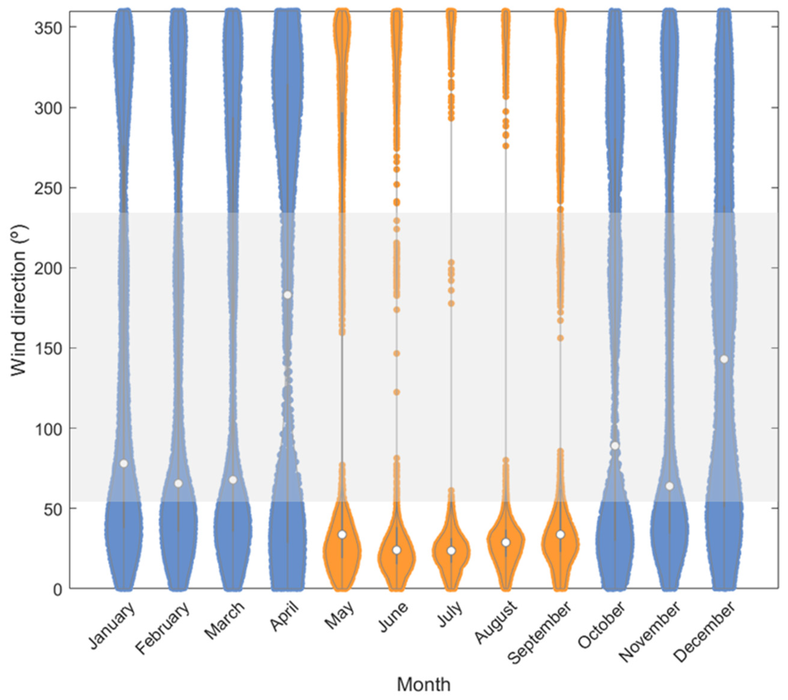
The distribution of monthly wind direction (above the dynamic threshold) is asymmetric when considering the months of May to September and October to April (Figure 3). During the former period, the wind blows almost exclusively from the north and northeast. During the latter period, there is a wide range of wind directions, with all octants represented. Throughout the year, the median wind direction is located between the north and east octants, except for the months of April and December when it shifts to the south and southeast.
4.2.2. Wind Regime for the Study Period
Data gathered in Table 4 show the wind variability in the time intervals covered by this study, the first interval corresponding to the wind conditions during the 6 months preceding the first field campaign. The period from October 2021 to May 2022 stands out for presenting slightly higher values of mean and maximum wind speed and the mean gust; moreover, the mean wind direction is from the northeast octant, in contrast to the other periods when the wind blew from the north. In this study, winter periods refer to the months between October and February (April or May), and summer periods refer to the months between April or May and October.
Prevailing winds were from the northern sectors, with the N and NE octants representing about 45 to 75% of the total occurrences, and higher frequencies in summer periods (Supplementary Materials, Figures S5–S7). NW winds are fairly constant and represent between 8 and 15% of occurrences, contributing to the rise of the percentage of northerlies up to 90%. Winds from the southern sectors (SE, S and SW octants) represent between 6 and 28% of the total occurrences, with higher representativeness in the winter periods. Similarly, winds from the E are more frequent in winter periods with 8 to 12% of occurrences compared to 1 to 3% in the other periods. Winds blowing from the west are more evenly distributed over all time intervals, ranging from 4 to 10%.
In summary, during summer periods, winds blew almost exclusively from the northern sectors, while during winter periods, a wide range of directions is observed, including winds from the southern sectors. On average, about 40% of the winds have transport potential, with the highest percentage generally blowing from the NE.
4.2.3. Potential Aeolian Transport
Estimates of potential sand transport between campaigns (Table 5) correspond to landward transport considering the onshore component of potential aeolian transport. Results highlight the seasonality associated with southerly and east winds and show that winter periods are the ones with significant potential for sand input to the foredune.
4.3. Vegetation
The changes in vegetation cover over time (Figure 4) are mainly related to the control of IAS, including their removal (leading to a decrease in vegetation cover) and the planting of autochthonous species (responsible for a limited increase in vegetation cover). Yellow dashed lines limit the SW, central and NE foredune sections.
These control actions started in April 2021 (after the April 2021 field campaign) and the main changes observed in the vegetation cover (Figure 4) were the following:
- From April 2021 to October 2021, there was a decrease in vegetation cover in the SW section of the foredune;
- From October 2021 to May 2022, there was vegetation growth in the same area above; significant removal of invasive vegetation occurred in the NE section of the foredune;
- From May 2022 to October 2022, there was some vegetation growth in the NE foredune section; repeated vegetation removal occurred in the SW foredune section. In the October 2022 orthomosaic, there is an apparent increase in vegetation cover in the central and SW sections of the leeward foredune slope, but this is largely an artifact associated with shaded areas.
- From October 2022 to February 2023, repeated vegetation removal led to a significant decrease in vegetation cover in both the SW and NE foredune sections.
4.4. Morphological Evolution and Sediment Budget
Results from the elevation differences models (Figure 5) reveal that most of the altimetric changes are less than or equal to 0.10 m, corresponding to the range of uncertainty associated with the surveys. Some areas of significant erosion and accretion (>1 m) are observed along the northern boundary of the models (matching the second dune) which may correspond to spurious results due to boundary effects (Figure 5, October 2020–April 2021). Similarly, significant erosion and accretion patterns can also be observed in association with small patches of shrubby vegetation.
In general, more significant altimetric variations were observed during the winter periods. Considering the two summer periods, the one between May and October 2022 shows practically no changes. It can be verified that in the first period (October 2020–April 2021), the spatial pattern of accretion/erosion distribution was not uniform with a dominance of accretion. In every other period, areas with both adjacent accretion/erosion patterns and with the same approximate shape and direction are identified, suggesting sediment movement associated with the shifting of sand bodies. In the last period (October 2022–February 2023) and especially in the NE sector of the foredune, there was a reversal in the signal of previous altimetric changes, with erosional areas becoming accretionary and vice versa.
Sediment budget between campaigns and per geomorphological unit is illustrated in Figure 6 and is expressed normalized by time (see Supplementary Materials, Table S2 for the corresponding areas).
Foredune accretion stands out, associated with both the October to April (May) winter periods in 2021 and 2022, corresponding to a mean increase in height of about +0.06 m at the end of each period. The remaining geomorphological units and time periods show very small volume changes, which were considered negligible, except for the deflation basin unit. In the first and fourth periods, the latter shows an increase in height of about +0.03 m at the end of each period.
Additionally, the sediment budget results per geomorphological unit over time were compared for both the total and bare sand areas to evaluate the impact of vegetation on evolution trends and budgets. The plot of volumetric changes in Figure 7 shows a strong linear trend when considering all data (R2 = 0.91). It should be noted that areas with more vegetation, such as the second dune and interdune, have slightly lower R2 values than less vegetated areas. These results suggest that the uncertainty related to vegetation height has no significant impact on the evolutionary trend or on the global budget when computing sediment budgets using (unmasked) DSM comparisons.
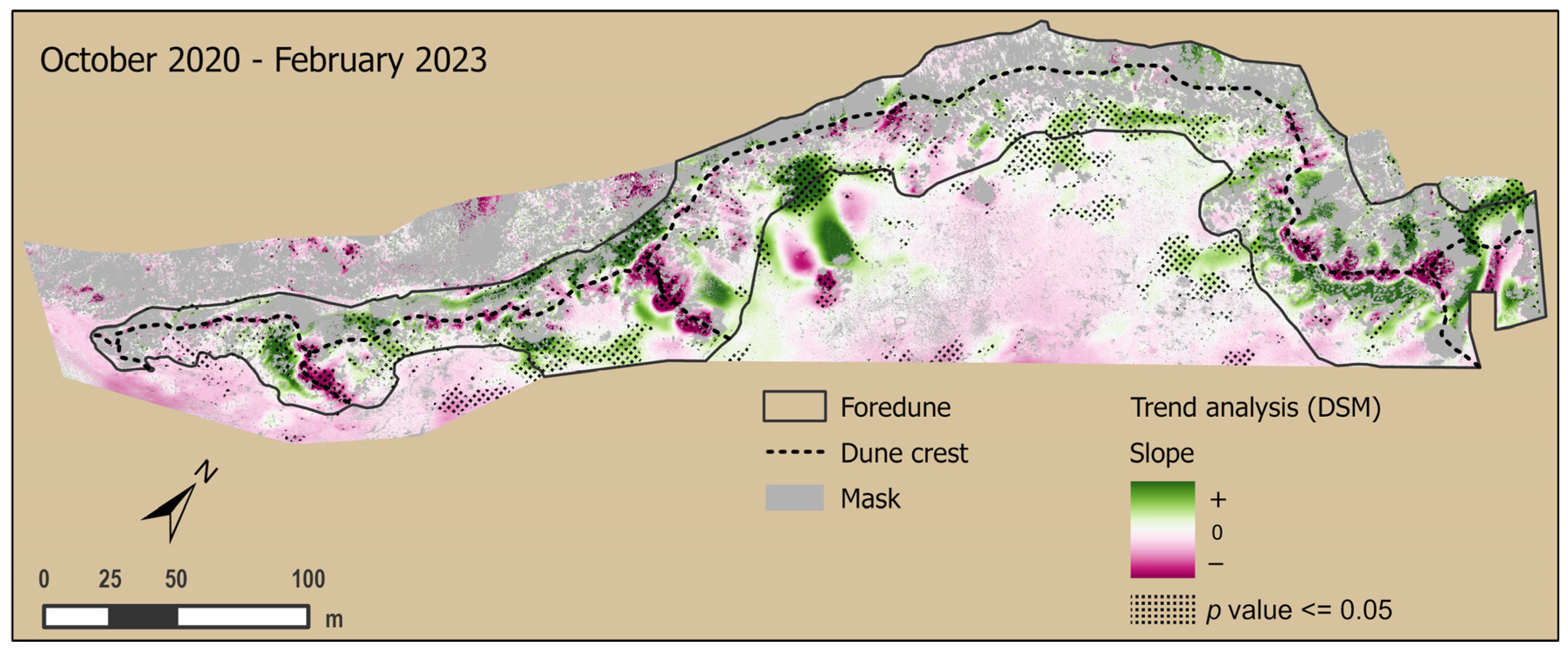
Regarding the spatial distribution of the short-term trends (Figure 8), the following patterns can be observed: (i) sediment movement towards the SW and W, almost parallel to the coastline, is observed in the foredune SW section, and these patterns are associated with two secondary crests showing nearly cross-shore elongation; (ii) strong evidence of sediment transfer towards the S is observed in the foredune NE section; (iii) the deflation basin exhibits a slight erosional tendency over its central region and accretion in the peripheral areas leaning towards the dune toe, with particular emphasis on the SW. The spatial distribution of the P statistic in Figure 8 indicates that these patterns generally correspond to values of p < 0.05, which reject the null hypothesis of random distribution. In this sense, interpreting a cause-and-effect relationship between vegetation removal and morphological variation induced by sand mobility becomes more coherent.
5. Discussion
5.1. Digital Surface Models and Sediment Budget
DSMs represent terrain elevation over unvegetated or scarcely vegetated areas, while in densely vegetated areas, DSMs represent canopy elevation rather than terrain (e.g., [34]). This issue may be relevant to the assessment of the dune volume, particularly if there are significant changes in the vegetation cover, as is the case in the present study. To remove this potential effect on the sediment budget results and on the assessment of morphological evolution trends, a mask was used to extract bare sand areas from all surveys. The removed area (vegetation, shadows and dark pebbles) represents 36% of the total area (~50 × 103 m2). However, the volume changes over time in the total area (vegetated and bare sand areas) show the same trends with proportional budgets (Figure 7). There were two periods of significant foredune accretion associated with the first two of the three winter periods. The remaining geomorphological units revealed very low or negligible budgets.
5.2. Wind Regime and Foredune Sediment Budget
Prevailing winds blow from the northern sectors. The direction of the coast under study is ~50°N and the beach–dune system is facing southeast, which means that the prevailing winds blow seawards. As the surface adjacent to the dune and extending landwards is completely vegetated and consists of colluvium, sand inputs from the northern sectors to the beach–dune system are not expected. Winds from the southern sectors with an onshore component, and especially those with speed above the dynamic threshold, blow almost exclusively during winter periods, showing seasonality (Figure 3, and Figures S5–S7 in Supplementary Materials).
Among the winds with transport potential, the NE octant (22.5°N to 67.5°N), which contains the coastline trend, contributes with the highest number of occurrences. However, although obliquely oriented winds result in larger effective fetch distances [43,44], only a small fraction of the northeasterly winds have an onshore component. Thus, NE winds are too oblique with respect to the general foredune and coastal alignment and have a reduced contribution to the foredune sediment input. Our data (Table 5) indicate that the NE potential sand input averages 5% of the total during winter periods. During summer periods, the NE potential sand input ranges from 38 to 72% of an extremely small total. Oblique winds blowing from southern (S and SW) and E octants, although less frequent, also benefit from larger fetch. Their joint potential for onshore sand transport averages 70% of the total in each winter period. During the summer periods, this potential drops to an average of 14% of an extremely small total, with no contribution of easterlies. In addition, SE winds in winter contribute 25% to the potential sand input but have no contribution in summer. The above discussion highlights the strong asymmetry in potential sand input (Table 5) related to the seasonality of the wind regime, with sediment input potential differing by one to two orders of magnitude. This is consistent with the sediment budget results estimated from the volume differences between DSMs (Figure 6).
During the last winter period (October 2022–February 2023), no significant sediment input to the foredune was observed (Figure 6), which contrasts with the magnitude of the budget verified in the two previous winter periods: the former is only about 15% of the latter. This may be related to the shortened duration of the last period, as the months of March, and especially April, typically have more winds blowing from the southern sectors (Figure 3).
5.3. Wind Regime, Sediment Movement and Vegetation
Assessment of the short-term evolution of the Porto Santo foredune using the trend analysis tool highlighted sediment movement patterns associated with prevailing winds, from the N and mainly the NE. It also revealed the importance of vegetation in sand retention. In the NE foredune section, significant vegetation removal triggered sand movement to the south, towards the beach, consistent with winds blowing from the N. In the SW section, sand movement occurred broadly parallel to the coastline, consistent with winds blowing from the NE. We interpret these differences in behavior as related to the effects of the surrounding morphology (cf. Supplementary Materials, Figure S1): (i) the NE section of the dune is located downwind of a N-S valley that is confined between the “Espigão” and “Ana Ferreira” peaks through which the prevailing winds are channeled; (ii) the remaining foredune sections are sheltered from N and NW winds by the “Zimbralinho” and “Espigão” reliefs, but they are more exposed to NE winds.
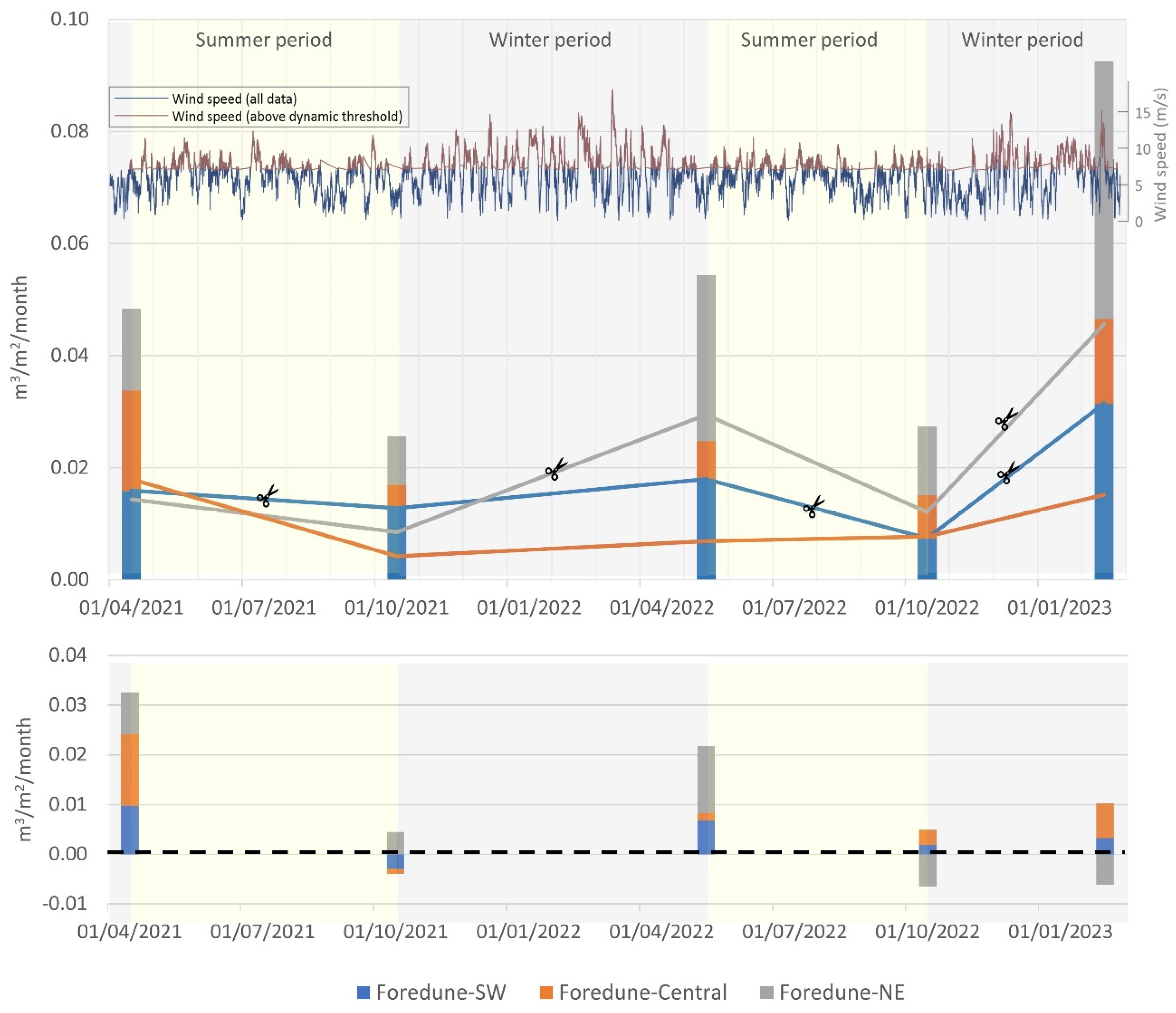
Gross volume changes were computed and compared to net volume changes, aiming at relating vegetation removal and sediment mobility over the different foredune sections (Figure 9). The stacked column on the left, representing a period without vegetation disturbance, shows a very similar behavior along the entire foredune length. In contrast, an increase in sediment mobility directly related to vegetation removal is observed. This effect is particularly strong in the NE section following both IAS removal interventions and is even more significant in the SW section during the last winter period, when the extension of IAS control was at its maximum. On the other hand, the central section, which was subjected to minimal intervention (not visible in Figure 4), has the lowest mobility. Figure 9 also shows differences in the magnitude of sediment mobility due to wind seasonality and that an increase in gross volume does not necessarily correspond to an increase in net volume, as also observed by [18].
In addition, we hypothesize that once the main trend of aeolian sediment movement is to the SW, related to the prevalence of effective NE winds, such a trend can result in a long-term loss of sediment (albeit of small magnitude) from the aeolian system to the beach. Once captured by the longshore drift current, beach sediment is lost to deep water at the SW corner of the island [19]. This represents an irreversible sink for the beach–dune system.
6. Conclusions
The morphological evolution of the Porto Santo dune results from an endless balance between sand supply, transport and retention. At the study site, the wind regime is asymmetric and dominated by offshore northerly winds, with potential to transport sand from the dune to the beach. However, the presence of vegetation makes the winds with an onshore component the primary agents responsible for conveying sand to the dune and promoting its development. These winds transfer sand from a non-vegetated source area (the beach), where it is easily mobilized, to a vegetated dune area, where it becomes retained. The findings from this study highlight that vegetation removal can expose dune sand to the predominant winds, potentially leading to its mobilization onto the beach and reducing the dune sand stock. As invasive species are increasingly recognized as threats to environmental and ecological stability in these systems, the need for IAS control operations has become more frequent. In light of the escalating frequency of IAS removal interventions, it becomes imperative to strategically time these interventions. This research advocates for conducting removal operations during the winter period when onshore winds dominate, as opposed to the summer when winds favor transport towards the sea. By aligning control efforts with seasonal wind conditions, there is an opportunity to minimize the risk of unintended consequences.
This research has significant implications for the management of dune vegetation control actions, especially those associated with IAS eradication in contexts where preventing increased mobility and preserving dune volume is crucial. Understanding the patterns of sediment mobility associated with the prevailing wind regimes is invaluable in devising effective restoration strategies and determining the optimal timing for their implementation. These findings emphasize the importance of considering sediment mobility patterns when planning vegetation control measures as part of dune restoration strategies.
Supplementary Materials
The following supporting information can be downloaded at https://www.mdpi.com/article/10.3390/rs16091487/s1. Figure S1: Porto Santo island, perspective to northeast. Yellow circle: study area (LIFE-Dunas project intervention area). Label refers to main peaks surrounding the study area. Figure S2: (A) Location of the GCPs used in the October 2020 UAV survey. GCP marking and RTK-GPS measurement of GCPs using (B) colored plastic plates, (C) sand marks or (D) marks with fluorescent biodegradable paint. Figure S3: Top: Illustration of the absolute altimetric deviations associated with all DSMs in the study area over ESRI Basemap and Feb 2023 orthomosaic. Bottom: Box-plot (left) and scatter diagram (right) of altimetric deviations between interpolated (DSM) and measured (RTK-GPS) homologous points. Figure S4: Wind data (between 1999 and Feb. 2023). Left—wind statistics: Fr (frequency of records); N (number of records); Vmax (maximum velocity); (mean velocity); (median velocity); P25 (velocity 25th percentile); P75 (velocity 75th percentile); (average gust); and (upwind vectorial mean direction). Right—scatter diagram of wind speed vs. gust. In red, linear fit to the data; linear equation and correlation coefficient (R2). Figure S5: Joint distribution of wind direction and speed between April 2020–October 2020 (top) and October 2020–April 2021 (bottom). Black dotted line represents coastline direction. Upper diagrams: all records. Lower diagrams: winds above dynamic threshold. Figure S6: Joint distribution of wind direction and speed between Apr 2021–October 2021 and October 2021–May 2022. Black dotted line represents coastline direction. Upper diagrams: all records. Lower diagrams: winds above dynamic threshold. Figure S7: Joint distribution of wind direction and speed between May 2022–October 2022 and October 2022–February 2023. Black dotted line represents coastline direction. Upper diagrams: all records. Lower diagrams: winds above dynamic threshold. Table S1: UAV flight dates; average flight altitude (m); overflown area (m2); number of images; number of measured GCPs. DSM and orthomosaic resolutions. Table S2: Total area and bare sand area (m2) per geomorphologic unit.
Author Contributions
A.P.B. led the study from early stages to the final manuscript, including field surveys, data acquisition, processing and interpretation. A.N.S. served as the Ph.D. supervisor for A.P.B., A.N.S. and R.T. and is the PI of the LIFE Dunas project supporting this study. A.N.S., R.T. and C.A. closely collaborated in data acquisition. A.N.S. and C.P.L. contributed to data processing. All authors contributed to the development of this study and were actively involved in data interpretation and discussions that resulted in the present study; also, they were engaged in editing, revising and approving the manuscript. All authors have read and agreed to the published version of the manuscript.
Funding
The authors acknowledge that this work was partially funded by the EU LIFE programme via project LIFE DUNAS (LIFE 19 CCA/PT/001178). The research was partially funded by the Portuguese Fundação para a Ciência e a Tecnologia (FCT) I.P./MCTES through national funds PIDDAC—UIDB/50019/2020: https://doi.org/10.54499/UIDB/50019/2020, https://doi.org/10.54499/UIDP/50019/2020 and LA/P/0068/2020: https://doi.org/10.54499/LA/P/0068/2020; A.N.S. was funded by DL57/2016/CP1479/CT0073: https://doi.org/10.54499/DL57/2016/CP1479/CT0073; and C.P.L. by DL57/2016/CP1479/CT0079: https://doi.org/10.54499/DL57/2016/CP1479/CT0079.
Data Availability Statement
The original contributions presented in the study are included in the article and Supplementary Materials, further inquiries can be directed to the corresponding author. The raw data supporting the conclusions of this article will be made available by the authors on request.
Conflicts of Interest
The authors declare no conflicts of interest. The funders had no role in the design of the study; in the collection, analyses, or interpretation of data; in the writing of the manuscript; or in the decision to publish the results.
References
- Hesp, P. Foredunes and blowouts: Initiation, geomorphology and dynamics. Geomorphology 2002, 48, 245–268. Available online: https://www.sciencedirect.com/science/article/pii/S0169555X02001848 (accessed on 12 May 2023). [CrossRef]
- Davidson-Arnott, R.; Hesp, P.; Ollerhead, J.; Walker, I.; Bauer, B.; Delgado-Fernandez, I.; Smyth, T. Sediment budget controls on foredune height: Comparing simulation model results with field data. Earth Surf. Process. Landf. 2018, 43, 1798–1810. [Google Scholar] [CrossRef]
- Zhu, X.; Linham, M.M.; Nicholls, R.J. Technologies for Climate Change Adaptation: Coastal Erosion and Flooding; TNA Guidebook Series; Danmarks Tekniske Universitet, Risø Nationallaboratoriet for Bæredygtig Energi: Kongens Lyngby, Denmark, 2010; Available online: https://orbit.dtu.dk/en/publications/technologies-for-climate-change-adaptation-coastal-erosion-and-fl (accessed on 2 June 2023).
- Hilgendorf, Z.; Walker, I.J.; Pickart, A.J.; Turner, C.M. Dynamic restoration and the impact of native versus invasive vegetation on coastal foredune morphodynamics, Lanphere Dunes, California, USA. Earth Surf. Process. Landf. 2022, 47, 3083–3099. [Google Scholar] [CrossRef]
- Temmerman, S.; Meire, P.; Bouma, T.J.; Herman, P.M.J.; Ysebaert, T.; de Vriend, H.J. Ecosystem-based coastal defence in the face of global change. Nature 2013, 504, 79–83. [Google Scholar] [CrossRef] [PubMed]
- Jackson, D.W.T.; Costas, S.; González-Villanueva, R.; Cooper, A. A global ‘greening’ of coastal dunes: An integrated consequence of climate change? Glob. Planet. Change 2019, 182, 103026. [Google Scholar] [CrossRef]
- Fabbri, S.; Grottoli, E.; Armaroli, C.; Ciavola, P. Using high-spatial resolution UAV-derived data to evaluate vegetation and geomorphological changes on a dune field involved in a restoration endeavour. Remote Sens. 2021, 13, 1987. [Google Scholar] [CrossRef]
- Murray, N.J.; Phinn, S.R.; DeWitt, M.; Ferrari, R.; Johnston, R.; Lyons, M.B.; Clinton, N.; Thau, D.; Fuller, R.A. The global distribution and trajectory of tidal flats. Nature 2019, 565, 222–225. [Google Scholar] [CrossRef] [PubMed]
- Martínez, M.L.; Hesp, P.A.; Gallego-Fernández, J.B. Coastal Dune Restoration: Trends and Perspectives. In Restoration of Coastal Dunes; Martínez, M., Gallego-Fernández, J., Hesp, P., Eds.; Springer Series on Environmental Management; Springer: Berlin/Heidelberg, Germany, 2013. [Google Scholar] [CrossRef]
- Thomas, Z.A.; Turney, C.S.M.; Palmer, J.G.; Lloydd, S.; Klaricich, J.N.L.; Hogg, A. Extending the observational record to provide new insights into invasive alien species in a coastal dune environment of New Zealand. App. Geogr. 2018, 98, 100–109. [Google Scholar] [CrossRef]
- Šilc, U.; Stešević, D.; Rozman, A.; Caković, D.; Küzmič, F. Alien species and the impact on sand dunes along the NE Adriatic coast. In Impacts of Invasive Species on Coastal Environments; Makowski, C., Finkl, C., Eds.; Springer, Coastal Research Library: Berlin/Heidelberg, Germany, 2019; Volume 29, pp. 113–143. Available online: https://link.springer.com/chapter/10.1007/978-3-319-91382-7_4 (accessed on 24 November 2022).
- Pickart, A.J. Ammophila invasion ecology and dune restoration on the west coast of north America. Diversity 2021, 13, 629. [Google Scholar] [CrossRef]
- Ruessink, B.G.; Arens, S.M.; Kuipers, M.; Donker, J.J.A. Coastal dune dynamics in response to excavated foredune notches. Aeol. Res. 2018, 31, 3–17. [Google Scholar] [CrossRef]
- Jackson, N.L.; Nordstrom, K.F.; Feagin, R.A.; Smith, W.K. Coastal geomorphology and restoration. Geomorphology 2013, 199, 1–7. [Google Scholar] [CrossRef]
- Delgado-Fernandez, I.; Davidson-Arnott, R.G.D.; Hesp, P.A. Is ‘re-mobilisation’ nature restoration or nature destruction? A commentary. J. Coast. Conserv. 2019, 23, 1093–1103. [Google Scholar] [CrossRef]
- Psuty, N.P.; Silveira, T.M. Restoration of Coastal Foredunes, a Geomorphological Perspective: Examples from New York and from New Jersey, USA. In Restoration of Coastal Dunes; Martínez, M.L., Gallego-Fernández, J.B., Hesp, P.A., Eds.; Springer: Berlin/Heidelberg, Germany, 2013; pp. 33–47. [Google Scholar] [CrossRef]
- Darke, I.B.; Walker, I.J.; Hesp, P.A. Beach–dune sediment budgets and dune morphodynamics following coastal dune restoration, Wickaninnish Dunes, Canada. Earth Surf. Process. Landf. 2016, 41, 1370–1385. [Google Scholar] [CrossRef]
- Caster, J.; Sankey, J.B.; Sankey, T.T.; Kasprak, A.; Bowker, M.A.; Joyal, T. Do topographic changes tell us about variability in aeolian sediment transport and dune mobility? Analysis of monthly to decadal surface changes in a partially vegetated and biocrust covered dune field. Geomorphology 2024, 447, 109021. [Google Scholar] [CrossRef]
- Silva, A.N.; Taborda, R.; Andrade, C.; Ribeiro, M. The future of insular beaches: Insights from a past-to-future sediment budget approach. Sci. Total Environ. 2019, 676, 692–705. [Google Scholar] [CrossRef] [PubMed]
- AEMET-IM. Climate Atlas of the Archipelagos of the Canary Islands, Madeira and the Azores. 2012. Available online: https://www.ipma.pt/export/sites/ipma/bin/docs/publicacoes/atlas.clima.ilhas.iberico.2011.pdf (accessed on 20 March 2021).
- Andrade, C.; Freitas, M.C.; Taborda, R.; Prada, S. Project: Plano de Urbanização para a Frente de Mar, Campo de Baixo/Ponta da Calheta, Porto Santo, Relatório 1a Fase, Caracterização e Diagnóstico. Anexo 1—Geologia, Geomorfologia Costeira, Dinâmica Costeira, Hidrogeologia; Unpublished Technical Report; Faculdade de Ciências da Universidade de Lisboa/Universidade da Madeira/Bruno Soares–Arquitectos, Lda.: Lisboa, Portugal, 2008; Available online: https://docplayer.com.br/77116599-Plano-de-urbanizacao-da-frente-mar-campo-de-baixo-ponta-da-calheta-porto-santo-1a-fase-caracterizacao-e-diagnostico.html (accessed on 10 September 2023). (In Portuguese)
- Silva, J.B. Areia de Praia da ilha de Porto Santo, Geologia, Génese, Dinâmica e Propriedades Medicinais. Ph.D. Thesis, Universidade de Aveiro, Aveiro, Portugal, 2002. (In Portuguese). [Google Scholar]
- Andrade, C.; Taborda, R.; Ribeiro, M.; Silva, A.N. Estudo da Dinâmica Sedimentar da Praia de Porto Santo; Unpublished Technical Report; Fundação da Faculdade de Ciências da Universidade de Lisboa/Governo Regional da Madeira: Lisboa, Portugal, 2017. (In Portuguese) [Google Scholar]
- Fernandes, F.; Medeiros, C.; Martins, A.; Freitas, S.; Abreu, F. Atualização da Cobertura Ecológica da Área de Intervenção do Projeto; LIFE Dunas Project (LIFE19 CCA/PT/001178) Unpublished Technical Report; Região Autónoma da Madeira Portugal, 2023. Available online: https://lifedunas.madeira.gov.pt/index.php/resultados/relatorios (accessed on 20 December 2023)(In Portuguese, abstract in English).
- Freitas, S.; Martins, A.; Medeiros, C.; Abreu, F.; Fernandes, F. Plano Operacional para Restauração de Habitats; LIFE Dunas Project (LIFE19 CCA/PT/001178) Unpublished Technical Report; Região Autónoma da Madeira Portugal, 2023. Available online: https://lifedunas.madeira.gov.pt/index.php/resultados/relatorios (accessed on 20 December 2023)(In Portuguese, abstract in English).
- Marchante, H.; Morais, M.; Freitas, H.; Marchante, E. Guia Prático para a Identificação de Plantas Invasoras em Portugal; Imprensa da Universidade de Coimbra: Coimbra, Portugal, 2014. [Google Scholar] [CrossRef]
- Abreu, F. Relatório de Progresso, Projeto LIFE Dunas (LIFE19 CCA/PT/001178); Unpublished Technical Report; LIFE Dunas: Madeira, Portugal, 2022; (In Portuguese, abstract in English). [Google Scholar]
- Jardim, R.; Sequeira, M.; Capelo, J.; Aguiar, C.; Costa, J.C.; Espírito Santo, M.D.; Lousã, M. Notas do herbário da Estação Florestal Nacional, XXXVI: The vegetation of Madeira: IV—Coastal Vegetation of Porto Santo Island (Archipelago of Madeira). Silva Lusit. 2003, 11, 116–120. [Google Scholar]
- Abreu, D.A.; Abreu, C.; Jardim, R.; Araúlo, R.; Abreu, U. Project: Plano de Urbanização para a Frente de Mar, Campo de Baixo/Ponta da Calheta, Porto Santo. Relatório 1a Fase, Caracterização e Diagnóstico. Anexo 7—Ecologia—Fauna e Flora Terrestres e Marinha; Unpublished Technical Report; GaiaWare/Bruno Soares—Arquitectos, Lda.: Lisboa, Portugal, 2008. (In Portuguese) [Google Scholar]
- Mancini, F.; Dubbini, M.; Gattelli, M.; Stecchi, F.; Fabbri, S.; Gabbianelli, G. Using unmanned aerial vehicles (UAV) for high-resolution reconstruction of topography: The structure from motion approach on coastal environments. Remote Sens. 2013, 5, 6880–6898. [Google Scholar] [CrossRef]
- Gonçalves, J.A.; Henriques, R. UAV photogrammetry for topographic monitoring of coastal areas. J. Photogram Remote Sens. 2015, 104, 101–111. [Google Scholar] [CrossRef]
- Casella, E.; Rovere, A.; Pedroncini, A.; Stark, C.P.; Casella, M.; Ferrari, M.; Firpo, M. Drones as tools for monitoring beach topography changes in the Ligurian Sea (NW Mediterranean). Geo-Mar. Lett. 2016, 36, 151–163. [Google Scholar] [CrossRef]
- Long, N.; Millescamps, B.; Pouget, F.; Dumon, A.; Lachaussee, N.; Bertin, X. Accuracy assessment of coastal topography derived from UAV images. The International Archives of the Photogrammetry. Remote Sens. Spat. Inf. Sci. 2016, 41, 1127–1134. [Google Scholar] [CrossRef]
- Taddia, Y.; Corbau, C.; Zambello, E.; Russo, V.; Simeoni, U.; Russo, P.; Pellegrinelli, A. UAVs to assess the evolution of embryo dunes. International Archives of the Photogrammetry. Remote Sens. Spat. Inf. Sci. 2017, 42, 363–369. [Google Scholar] [CrossRef]
- Bastos, A.P.; Lira, C.P.; Calvão, J.; Catalão, J.; Andrade, C.; Pereira, A.J.; Taborda, R.; Rato, D.; Pinho, P.; Correia, O. UAV derived information applied to the study of slow-changing morphology in dune systems. J. Coast. Res. 2018, 85, 226–230. [Google Scholar] [CrossRef]
- Hilgendorf, Z.; Marvin, M.C.; Turner, C.M.; Walker, I.J. Assessing geomorphic change in restored coastal dune ecosystems using a multi-platform aerial approach. Remote Sens. 2021, 13, 354. [Google Scholar] [CrossRef]
- Ullman, S. The interpretation of structure from motion. Proc. R. Soc. Lond. B 1979, 203, 405–426. Available online: https://royalsocietypublishing.org/ (accessed on 17 December 2022). [PubMed]
- Eltner, A.; Kaiser, A.; Castillo, C.; Rock, G.; Neugirg, F.; Abellán, A. Image-based surface reconstruction in geomorphometry-merits, limits and developments. Earth Surf. Dyn. 2016, 4, 359–389. [Google Scholar] [CrossRef]
- Hersbach, H.; Dee, D. Reanalysis Is in Production. Available online: https://www.ecmwf.int/en/newsletter/147/news/era5-reanalysis-production (accessed on 2 August 2022).
- Bagnold, R. The Physics of Blown Sand and Desert Dunes, 1st ed.; Chapman and Hall: London, UK, 1941. [Google Scholar]
- Van Rijn, L. Aeolian Transport over a Flat Sediment Surface. Available online: https://www.leovanrijn-sediment.com/papers/Aeoliansandtransport2018.pdf (accessed on 2 March 2018).
- Faelga, R.A.; Cantelli, L.; Silvestri, S.; Giambastiani, B.M.S. Dune belt restoration effectiveness assessed by UAV topographic surveys (northern Adriatic coast, Italy). Biogeosciences 2023, 20, 4841–4855. [Google Scholar] [CrossRef]
- Bauer, B.O.; Davidson-Arnott, R.G.D.; Hesp, P.A.; Namikas, S.L.; Ollerhead, J.; Walker, I.J. Aeolian sediment transport on a beach: Surface moisture, wind fetch, and mean transport. Geomorphology 2009, 105, 106–116. [Google Scholar] [CrossRef]
- Delgado-Fernandez, I. A review of the application of the fetch effect to modelling sand supply to coastal foredunes. Aeol. Res. 2010, 2, 61–70. [Google Scholar] [CrossRef]
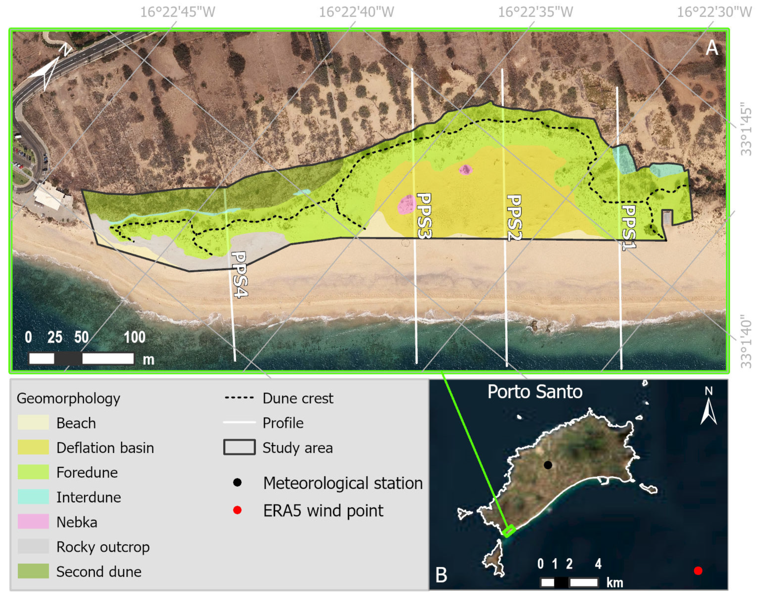
Figure 1.
(A)—Location of the study area with control cross-shore profiles (PPS1 to PPS4) and geomorphological units (see explanation in text). DGT orthophotomap. (B)—Porto Santo island with the location of the study area (green), the ERA5 wind data extraction point (red dot; 16.25°W, 33.00°N) and the airport meteorological station (black dot; 16.35°W, 33.07°N).

Figure 2.
Views to the northeast of the interdune area in the southwest dune section before (left photo) and after the removal (right photo) of A. donax and C. edulis. Photos: courtesy of IFCN.
Figure 2.
Views to the northeast of the interdune area in the southwest dune section before (left photo) and after the removal (right photo) of A. donax and C. edulis. Photos: courtesy of IFCN.

Figure 3.
Violin diagram showing the monthly distribution of wind direction (above the dynamic threshold). Shaded (unshaded) areas correspond to winds with an onshore (offshore) component. Orange (blue) indicates months with a lower (higher) frequency of onshore winds.
Figure 3.
Violin diagram showing the monthly distribution of wind direction (above the dynamic threshold). Shaded (unshaded) areas correspond to winds with an onshore (offshore) component. Orange (blue) indicates months with a lower (higher) frequency of onshore winds.

Figure 4.
Orthomosaics’ classification rasters. The bands colored in green indicate the foredune sections that underwent vegetation removal (dark green) or had no intervention (light green). Yellow dashed lines limit SW, central and NE foredune sections.
Figure 4.
Orthomosaics’ classification rasters. The bands colored in green indicate the foredune sections that underwent vegetation removal (dark green) or had no intervention (light green). Yellow dashed lines limit SW, central and NE foredune sections.

Figure 5.
Elevation differences model in the study area showing sediment erosion (orange and red tones) and accretion (green tones) between campaigns; colorless represents changes within 0.10 m. UAV orthomosaic over ESRI Basemap.
Figure 5.
Elevation differences model in the study area showing sediment erosion (orange and red tones) and accretion (green tones) between campaigns; colorless represents changes within 0.10 m. UAV orthomosaic over ESRI Basemap.

Figure 6.
Volume differences (m3/month) per geomorphological units, considering the total area (green columns) and the bare sand area (yellow columns).
Figure 6.
Volume differences (m3/month) per geomorphological units, considering the total area (green columns) and the bare sand area (yellow columns).

Figure 7.
Plot of volume differences (m3/month) per geomorphological unit calculated for the total area vs. the bare sand area.
Figure 7.
Plot of volume differences (m3/month) per geomorphological unit calculated for the total area vs. the bare sand area.

Figure 8.
Short-time trend analysis maps: slope plot of the linear trend corresponding to the best-fit line between the DSM values over time; p value statistic < 0.05 indicated by black dotted pattern. Mask (in gray) corresponds to areas that were classified as “no data”.
Figure 8.
Short-time trend analysis maps: slope plot of the linear trend corresponding to the best-fit line between the DSM values over time; p value statistic < 0.05 indicated by black dotted pattern. Mask (in gray) corresponds to areas that were classified as “no data”.

Figure 9.
Top panel—Gross volume changes between consecutive campaigns per foredune section (SW, blue; central, orange; NE, gray), considering only the bare sand area. The stacked column on the left corresponds to changes measured between 13 October 2020 and 7 April 2021 (date format dd/mm/yyyy). Lines represent the progression of gross volume changes and scissors indicate vegetation control actions in each foredune section. Background color represents contrasting wind regimes (summer, in yellow; winter, in gray). The graph superimposed on top represents wind speed. Bottom panel—Net volume changes. The dashed black line marks the null budget.


Table 1.
Error statistics for the GCPs in the surveyed areas.
| Campaign | (m) | (m) | (m) | N | UAV Survey Area (m2) |
|---|---|---|---|---|---|
| October 2020 | 0.077 | 0.032 | 0.083 | 27 | 133,000 |
| April 2021 | 0.031 | 0.004 | 0.031 | 27 | 160,000 |
| October 2021 | 0.027 | 0.006 | 0.028 | 26 | 112,000 |
| May 2022 | 0.031 | 0.008 | 0.032 | 37 | 155,000 |
| October 2022 | 0.015 | 0.006 | 0.016 | 28 | 123,000 |
| February 2023 | 0.008 | 0.002 | 0.008 | 22 | 145,000 |
Table 2.
Elevation deviations (m) between modeled (DSM) and measured (RTK-GPS) independent validation points in the study area per campaign. Std—standard deviation; RMSE—root mean square error; N—number of points.
Table 2.
Elevation deviations (m) between modeled (DSM) and measured (RTK-GPS) independent validation points in the study area per campaign. Std—standard deviation; RMSE—root mean square error; N—number of points.
| Campaign | (m) | (m) | (m) | N |
|---|---|---|---|---|
| October 2020 | 0.06 | 0.01 | 0.09 | 398 |
| April 2021 | 0.08 | 0.05 | 0.10 | 306 |
| October 2021 | 0.05 | 0.05 | 0.09 | 316 |
| May 2022 | 0.05 | 0.05 | 0.08 | 299 |
| October 2022 | 0.05 | 0.06 | 0.08 | 717 |
| February 2023 | 0.05 | 0.06 | 0.08 | 305 |
| All data | 0.06 | 0.05 | 0.08 | 2341 |
Table 3.
Elevation deviations (m) between modeled (DSM) and measured (RTK-GPS) independent validation points in the study area per geomorphological unit and for bare sand in all units. Std—standard deviation; RMSE—root mean square error; N—number of points.
Table 3.
Elevation deviations (m) between modeled (DSM) and measured (RTK-GPS) independent validation points in the study area per geomorphological unit and for bare sand in all units. Std—standard deviation; RMSE—root mean square error; N—number of points.
| Geomorphological Unit | (m) | (m) | (m) | N |
|---|---|---|---|---|
| Deflation basin | 0.04 | 0.04 | 0.07 | 979 |
| Foredune | 0.07 | 0.06 | 0.11 | 849 |
| Interdune | 0.04 | 0.03 | 0.07 | 116 |
| Nebka | 0.03 | 0.01 | 0.05 | 48 |
| Rocky outcrop | 0.04 | 0.01 | 0.05 | 228 |
| Second dune | 0.06 | 0.04 | 0.08 | 121 |
| Bare sand (all units) | 0.007 | 0.04 | 0.07 | 1672 |
Table 4.
ERA 5 wind data characteristics per time intervals under study. N (number of records); (mean velocity); (median velocity); Umax (maximum velocity); (average gust); and (upwind vectorial mean direction).
Table 4.
ERA 5 wind data characteristics per time intervals under study. N (number of records); (mean velocity); (median velocity); Umax (maximum velocity); (average gust); and (upwind vectorial mean direction).
| Statistics | ERA5 Wind Data Per Time Interval | |||||
|---|---|---|---|---|---|---|
| April 2020–October 2020 | October 2020–April 2021 | April 2021–October 2021 | October 2021–May 2022 | May 2022–October 2022 | October 2022–February 2023 | |
| N | 4392 | 4224 | 4368 | 5232 | 3672 | 3264 |
| (m/s) | 6.2 | 6.2 | 6.2 | 7.0 | 6.0 | 6.1 |
| (m/s) | 6.5 | 5.9 | 6.5 | 6.9 | 6.3 | 6.1 |
| Umax (m/s) | 14.4 | 17.8 | 12.4 | 18.1 | 11.5 | 15.1 |
| (m/s) | 8.4 | 8.5 | 8.5 | 9.4 | 8.2 | 8.5 |
| (°) | 10.4 | 19.5 | 7.6 | 33.3 | 4.7 | 18.4 |
Table 5.
Potential aeolian transport in each time period estimated with the Bagnold [40] formula, considering only winds with an onshore component. N, total number of records. Shaded cells indicate winter periods.
Table 5.
Potential aeolian transport in each time period estimated with the Bagnold [40] formula, considering only winds with an onshore component. N, total number of records. Shaded cells indicate winter periods.
| Time Period | Octant | Total Potential Aeolian Transport (m3) | Time Normalized Potential Aeolian Transport (m3/month) | % Total |
|---|---|---|---|---|
| October 2020–April 2021 (N = 4224) | NE | 43 | 7 | 1 |
| E | 1178 | 201 | 31 | |
| SE | 619 | 106 | 16 | |
| S | 1538 | 262 | 40 | |
| SW | 427 | 73 | 11 | |
| Total | 3805 | 649 | 100 | |
| October 2021–October 2021 (N = 4368) | NE | 27 | 4 | 72 |
| E | 0 | 0 | 0 | |
| SE | 0 | 0 | 0 | |
| S | 4 | 1 | 11 | |
| SW | 6 | 1 | 17 | |
| Total | 38 | 6 | 100 | |
| October 2021–May 2022 (N = 5232) | NE | 321 | 44 | 5 |
| E | 1377 | 190 | 21 | |
| SE | 3337 | 459 | 51 | |
| S | 1134 | 156 | 17 | |
| SW | 392 | 54 | 6 | |
| Total | 6561 | 903 | 100 | |
| May 2022–October 2022 (N = 3672) | NE | 30 | 6 | 38 |
| E | 0 | 0 | 0 | |
| SE | 0 | 0 | 0 | |
| S | 22 | 4 | 28 | |
| SW | 27 | 5 | 34 | |
| Total | 79 | 15 | 100 | |
| October 2022–February 2023 (N = 3264) | NE | 135 | 30 | 10 |
| E | 228 | 50 | 18 | |
| SE | 89 | 20 | 7 | |
| S | 497 | 110 | 38 | |
| SW | 350 | 77 | 27 | |
| Total | 1299 | 287 | 100 |
Disclaimer/Publisher’s Note: The statements, opinions and data contained in all publications are solely those of the individual author(s) and contributor(s) and not of MDPI and/or the editor(s). MDPI and/or the editor(s) disclaim responsibility for any injury to people or property resulting from any ideas, methods, instructions or products referred to in the content. |
© 2024 by the authors. Licensee MDPI, Basel, Switzerland. This article is an open access article distributed under the terms and conditions of the Creative Commons Attribution (CC BY) license (https://creativecommons.org/licenses/by/4.0/).
Share and Cite
MDPI and ACS Style
Bastos, A.P.; Taborda, R.; Andrade, C.; Ponte Lira, C.; Nobre Silva, A. Short-Term Foredune Dynamics in Response to Invasive Vegetation Control Actions. Remote Sens. 2024, 16, 1487. https://doi.org/10.3390/rs16091487
AMA Style
Bastos AP, Taborda R, Andrade C, Ponte Lira C, Nobre Silva A. Short-Term Foredune Dynamics in Response to Invasive Vegetation Control Actions. Remote Sensing. 2024; 16(9):1487. https://doi.org/10.3390/rs16091487
Chicago/Turabian StyleBastos, Ana Pestana, Rui Taborda, César Andrade, Cristina Ponte Lira, and Ana Nobre Silva. 2024. "Short-Term Foredune Dynamics in Response to Invasive Vegetation Control Actions" Remote Sensing 16, no. 9: 1487. https://doi.org/10.3390/rs16091487
Note that from the first issue of 2016, this journal uses article numbers instead of page numbers. See further details here.