Article

Mapping Foliar C, N, and P Concentrations in An Ecological Restoration Area with Mixed Plant Communities Based on LiDAR and Hyperspectral Data

1
School of Environment and Spatial Informatics, China University of Mining and Technology, Xuzhou 221008, China
2
Engineering Research Center of Ministry of Education for Mine Ecological Restoration, China University of Mining and Technology, Xuzhou 221008, China
3
School of Public Administration, Hohai University, Nanjing 211100, China
*
Author to whom correspondence should be addressed.
Remote Sens. 2024, 16(9), 1624; https://doi.org/10.3390/rs16091624
Submission received: 16 March 2024 / Revised: 27 April 2024 / Accepted: 29 April 2024 / Published: 2 May 2024

Abstract

:
Interactions between carbon (C), nitrogen (N), and phosphorus (P), the vital indicators of ecological restoration, play an important role in signaling the health of ecosystems. Rapidly and accurately mapping foliar C, N, and P is essential for interpreting community structure, nutrient limitation, and primary production during ecosystem recovery. However, research on how to rapidly map C, N, and P in restored areas with mixed plant communities is limited. This study employed laser imaging, detection, and ranging (LiDAR) and hyperspectral data to extract spectral, textural, and height features of vegetation as well as vegetation indices and structural parameters. Causal band, multiple linear regression, and random forest models were developed and tested in a restored area in northern China. Important parameters were identified including (1), for C, red-edge bands, canopy height, and vegetation structure; for N, textural features, height percentile of 40–95%, and vegetation structure; for P, spectral features, height percentile of 80%, and 1 m foliage height diversity. (2) R2 was used to compare the accuracy of the three models as follows: R2 values for C were 0.07, 0.42, and 0.56, for N they were 0.20, 0.48, and 0.53, and for P they were 0.32, 0.39, and 0.44; the random forest model demonstrated the highest accuracy. (3) The accuracy of the concentration estimates could be ranked as C > N > P. (4) The inclusion of LiDAR features significantly improved the accuracy of the C concentration estimation, with increases of 22.20% and 47.30% in the multiple linear regression and random forest models, respectively, although the inclusion of LiDAR features did not notably enhance the accuracy of the N and P concentration estimates. Therefore, LiDAR and hyperspectral data can be used to effectively map C, N, and P concentrations in a mixed plant community in a restored area, revealing their heterogeneity in terms of species and spatial distribution. Future efforts should involve the use of hyperspectral data with additional bands and a more detailed classification of plant communities. The application of this information will be useful for analyzing C, N, and P limitations, and for planning for the maintenance of restored plant communities.

1. Introduction

Intense levels of human activity, such as mining, have caused extensive vegetation removal or degradation in many areas [1,2]. In recent years, important ecological restoration efforts have gained popularity; for instance, the United Nations recently declared 2021–2030 as the decade for ecosystem restoration [3]. Vegetation, as a vital component in ecological restoration, plays a crucial role by contributing significantly to the structure and function of ecosystems [4,5]. To ensure the stability and resilience of a restored ecosystem, land managers usually employ a variety of species during revegetation with the goal of creating a mixed-species plant community. However, the restoration of vegetation on degraded land is often limited by nutrient deficiency, which hinders the process of ecological restoration [6]. Therefore, monitoring the nutrient levels and functions of an ecosystem has become important to ensure that these characteristics develop according to the expected recovery trajectory [7,8].
For a restored plant community, carbon (C), nitrogen (N), and phosphorus (P) constitute fundamental building blocks required for plant growth and development. Carbon is the most important element with the highest concentration in leaf dry matter, while N and P are essential nutrients for building plant structures [9,10,11]; these three elements serve as important indicators of ecological health. Their availability and stoichiometric ratios not only indicate the nature of conditions related to plant growth and community composition [12,13] but also reveal the nutrient dynamics and limitations of plants under changing climatic conditions [14,15,16]. Nutrient limitations, specifically in the form of C, N, and P limitations, can impede the absorption and utilization of nutrients by plants, affecting their growth rates, metabolic processes, and the decomposition of litter [17,18]. This, in turn, influences the overall health of a restored ecosystem. Therefore, for the assessment of ecosystem health, and to ensure the success of restoration efforts, it is imperative to conduct rapid monitoring of foliar C, N, and P concentrations in a mixed plant community within an ecological restoration area.
Recent monitoring and assessment of restoration efforts have focused more on vegetation coverage or greenness rather than on the chemical or biological indicators of vegetative conditions [19,20]. In particular, limited research is available on the rapid monitoring of C, N, and P in mixed plant communities within ecological restoration areas. Traditional extensive surveys of foliar concentrations of C, N, and P in the canopy are time-consuming and labor-intensive, making them impractical for the large-scale mapping of C, N, and P and applications employed in post-restoration management. In the recent two decades, remote sensing has been adopted as an efficient alternative monitoring method, providing a crucial means for the large-scale monitoring of plant growth and quantification of the biochemical properties of vegetation [21,22,23]. Unmanned Aerial Vehicle (UAV)-based laser imaging, detection, and ranging (LiDAR) and hyperspectral remote sensing are two advanced remote sensing technologies, each possessing unique advantages in acquiring surface information [24]. Specifically, LiDAR is characterized by a high level of accuracy and an ability to penetrate the canopy, providing high-resolution three-dimensional structural information. This technique enables the accurate and effective monitoring of plant communities in spatial dimensions [25]. Hyperspectral remote sensing offers rich spectral information, exhibiting high sensitivity to vegetation health and types, which is valuable for monitoring vegetation health and conducting biochemical composition studies [26]. It has been found from recent research progress that the integration of LiDAR and hyperspectral data has a strong capacity to enable the classification of vegetation and assessment of structural and morphology parameters, such as biomass, diversity, and canopy coverage [27,28]. In addition, the two technological methods have been successfully applied to assess biochemical parameters such as N and P. However, those application cases mainly focus on individual species such as phoenix trees [29], rice [30], apple trees [31], Phragmites communis [32], and maize [33]. Studies that discuss the feasibility of mapping the foliar C, N, and P of restored ecosystems with mixed plant communities are lacking. Considering that the combination of LiDAR and hyperspectral data may provide information about the chemical signal of different plants with various morphologies, this synergistic approach may contribute to a better understanding of spatial heterogeneity in C, N, and P among different plant communities and their responses to ecological restoration.
Therefore, the present study is an attempt to examine the possibility of using LiDAR and hyperspectral data in the spatial mapping of the C, N, and P concentrations in a mixed plant community of an ecological restoration area. The main research goals include the following: (1) to establish the optimal model for estimating foliar C, N, and P concentrations; (2) to investigate how the LiDAR and hyperspectral data could contribute to the estimation accuracy; and (3) to discuss the ability of LiDAR and hyperspectral data to reveal the heterogeneity of foliar C, N, and P across plant species and spatial regions. The research aims to serve as a reference for identifying C, N, and P nutrient limitations and assessing the health of an ecosystem.

2. Materials and Methods

2.1. Study Area

The study area is the Shendong Mining Area, which is close to Ordos City, Inner Mongolia, China (Figure 1). The average annual temperature and precipitation of the area are about 8.5 °C and 300–400 mm, respectively. The average elevation of the area is around 1250 m, with significant terrain fluctuations; the region has a typical arid and semi-arid plateau continental climate. The study area has an east–west length of approximately 2 km and a north–south width of about 300 m, covering an area of approximately 0.6 km2. Situated in the transitional zone between grassland and forest steppe, the original vegetation types include deciduous trees, shrubs, sandy-soil vegetation, and grassland.
Intensive coal mining in the study area has negatively impacted the original vegetation of the site. Consequently, ecological restoration measures, primarily focused on soil and water conservation as well as revegetation, were undertaken after the completion of mining activities in 2010. The central part of the restored ecological zone includes roads with the restored vegetation types on the roadsides mainly consisting of Populus spp. (mixed poplar), Camphor pine, Wild cherry, Prunus sibirica, Prunus humilis, Salix spp., Sea buckthorn, Caragana spp., Amorpha fruticosa, Artemisia oleifera, and Medicago sativa. Among these, Populus spp. and Pinus sylvestris have been planted with a certain degree of regularity across the landscape. Sea buckthorn has been extensively planted as an economically important species, primarily concentrated in the central part of the study area.

2.2. Data

2.2.1. Remote Sensing Data

Two types of remote sensing data, i.e., LiDAR data (LiAir 220) and hyperspectral images, were acquired from the DJI M600 (Dajiang Baiwang Technology Co., Ltd., Shenzhen, Guangdong, China) on 25 July 2022. July is the growing season for plants in the study area. Investigating the growth status of vegetation during this season can reflect the success of the ecological restoration. LiDAR data were acquired by a LiAir 220 UAV LiDAR system. A total of three flight routes were planned. The flight height was 90 m, the speed was 5 m/s, the horizontal field of view angle was 360°, the vertical field of view angle was greater than 20°, and the average point cloud density was 130 points/m2. The elevation of the study area was 1200–1296 m, and the number of echoes was two. The LiDAR 360 6.0 software was acquired from GreenValley International (Berkeley, CA, USA) and was used for preprocessing. The preprocessing included creating an aerial strip mosaic, point cloud registration, strip redundancy removal, noise removal, point cloud feature extraction, and point cloud classification [26]. First, mosaic the LiDAR data and then register to minimize the spatial position differences between the points. Then, remove the redundant point cloud data of the overlapping part of the strip and point cloud noise, and then divide the point cloud into ground and non-ground points. Finally, extract the point cloud data features. Before extracting the LiDAR features, it was necessary to normalize the LiDAR data by subtracting the elevation value Z of each point in the LiDAR point cloud data. Normalization can remove the influence of terrain fluctuations on the elevation value of the point cloud data.
Hyperspectral data were acquired by an S185 hyperspectral sensor (Cubert GmbH, Ulm, Germany). For the hyperspectral data, eight flight routes were set up to ensure full coverage of the area. The drone had a flight altitude of 140 m, a spatial resolution of 0.19 m, and a lateral overlap rate of 57%, flying a total of four sorties. The spectral range obtained during each flight was 398–1002 nm, with a total of 112 bands. During the data collection, sensor calibration was carried out using a standard diffuse reflection board, followed by atmospheric correction, geometric correction, band splicing and cropping, and image fusion. Next, ENVI 5.0 software (Research Systems, Inc., Boulder, CO, USA) was employed for hyperspectral image preprocessing mainly including radiometric calibration, atmospheric correction, geometric correction, noise and dimensionality reduction, aerial strip mosaicking, clipping, and band fusion [34].

2.2.2. Field Data

While acquiring remote sensing data, 60 sample plots were established for collecting plant community data. Within each sample plot, three 10 m × 10 m quadrats were created for trees, 5 m × 5 m quadrats for shrubs, and 1 m × 1 m quadrats for grasses. The spacing between quadrats was greater than 50 m. In addition, a 500 g sample of canopy leaves was collected from the canopy of the plant community in each quadrat. In total, 166 samples of plant leaves were collected.
Fresh leave samples were first cleaned with distilled water to remove dust, sediments, and other debris. After rinsing with deionized water, they were rinsed with 18.2 MΩ ultrapure water. Leaf samples were dried in a baking oven at 105 °C for 15–20 min and then dried at 80 °C for 10 h until a constant weight was reached. The dried leaf samples were ground and passed through a 100-mesh screen. Next, a 6 g sample of the leaf samples was ground prior to determining the C, N, and P concentrations. The potassium dichromate oxidation, Semi-Micro-Kjeldahl, and Mo-Sb colorimetric methods were used to determine the C, N, and P concentrations in the leaves, respectively [16]. Table 1 shows the maximum, minimum, mean, and standard deviation of foliar C, N, and P of the collected samples.
Figure 2 shows the C, N, and P concentrations of eight dominant plant communities including the Pinus sylvestris, Populus spp., Salix spp., Sea buckthorn, Artemisia oleifera, Amorpha fruticosa, Caragana spp., and Herbaceous spp. communities. No significant difference in C concentration was observed among the eight dominant plant types. Among them, Pinus sylvestris exhibited the highest C concentration, while the Populus spp. and Herbaceous spp. communities showed slightly lower C concentrations. Considerable variations were observed for N and P. Amorpha fruticosa and Caragana spp. demonstrated relatively high N concentrations, while Pinus sylvestris, Populus spp., and Herbaceous spp. had lower N concentrations. Artemisia oleifera showed the highest P concentration, while Pinus sylvestris and Herbaceous spp. had lower P concentrations.

2.3. Methods

2.3.1. Technical Process

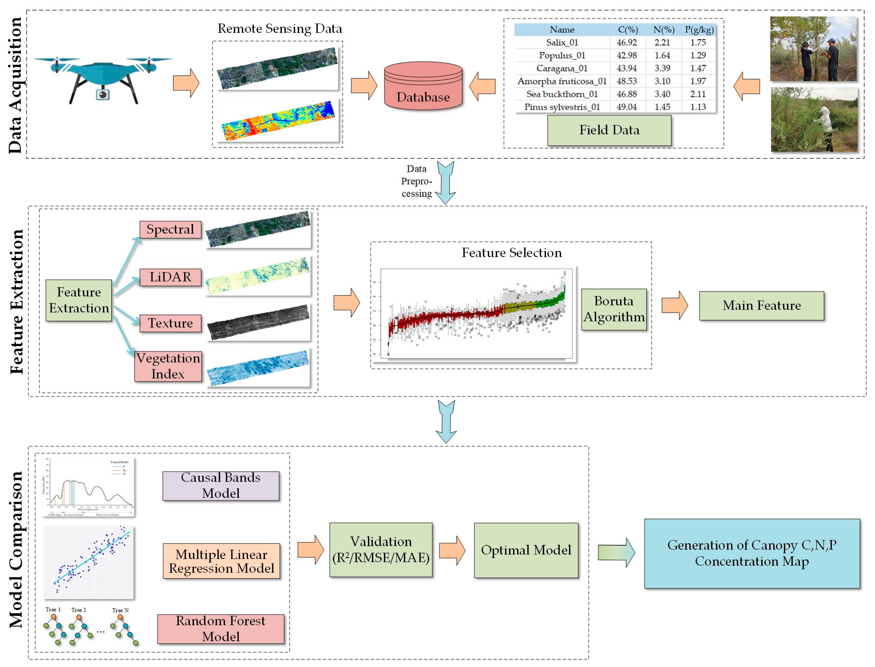
Figure 3 illustrates the technical roadmap for foliar C, N, and P mapping by using UAV-based LiDAR and hyperspectral data, combined with ground sampling data. The Boruta algorithm was used to select features and construct three models including causal bands (namely, causal absorption features (nm) related to foliar biochemicals including C, N, and P, multiple linear regression, and random forest. The model with the highest accuracy was used to map the foliar C, N, and P in the study area.

2.3.2. Extraction of Features

LiDAR can acquire the morphological characteristics of plant communities, and hyperspectral can reflect the spectral characteristics of different plant community types. The morphological point cloud filtering method [35] was used to distinguish the ground information in the LiDAR data and extract the variables highly correlated with the plant community. In this study, a total of 112 spectral features, 15 textural features, 33 vegetation indices, 34 height features, and seven vegetation structure parameters were extracted as parameters for model construction.
  • Spectrum
Given that the spectral reflectance of different plant leaves varies, 112 bands of hyperspectral data were employed as parameters for model construction. In this study, all 112 bands were used, with a wavelength range of 398–1002 nm and a band width of 5.2 nm.
2.
Texture
Mean, variance, entropy, data range, and skewness were extracted as textural features. Table 2 presents the calculation formulas for these features. Using ENVI’s Minimum Noise Fraction to process hyperspectral images, the first two converted bands contained more than 99% of the image information. In addition, green, red, and near-infrared bands are composed into a pseudo-color image synthesis band. These three bands were individually used to extract the five textural features in Table 2. In total, 15 textural features were extracted. The formula for calculating the pseudo-color image is as follows [26]:
B p s e u d o c o l o r = ( B G r e e n + B R e d + B N I R ) / 3
3.
Vegetation indices
Remote sensing-based vegetation indices can be used to qualitatively evaluate vegetation coverage and growth. Therefore, the 33 vegetation indices listed in Table 3 were selected for model construction.
4.
Height and vegetation structure parameters
The airborne LiDAR system can obtain a dense point cloud, from which the height and vegetation structure parameters can be extracted. In this study, 34 height features and seven vegetation structure parameters were selected, as shown in Table 4.

2.3.3. Selection of Features

Feature filtering refers to reducing the dimensionality of high-dimensional feature datasets by removing some invalid features, selecting the most suitable features for modeling, and constructing an optimal feature dataset. In general, feature filtering is required when a feature dataset is too large; this process not only reduces the computation time but also prevents the model from overfitting. In this study, the Boruta algorithm was used for feature selection [61]. This algorithm is designed as a wrapper around a random forest classification algorithm. It iteratively removes the features that are proven by a statistical test to be less relevant than random probes.
The Boruta algorithm consists of the following steps [61]:
  • Build random forest: construct a random forest model using the original dataset. This typically involves multiple decision trees, each trained on a random subset.
  • Calculate the importance of the original features: for each feature, compute its relative importance using the random forest model. This is achieved by measuring the contribution of the feature to the model’s predictive accuracy.
  • Create shadow features: for each original feature, generate a corresponding “shadow” feature. A shadow feature is created by randomly permuting the values of the original feature.
  • Build an extended random forest: build another random forest model using a dataset that includes both the original and shadow features.
  • Compute the importance of the shadow features: calculate the relative importance of each shadow feature in the extended random forest.
  • Compare the importance of the original and shadow features: for each original feature, compare its actual importance with the average importance of its shadow features. If the original feature’s importance is higher than the average importance of its shadow features, retain the feature; otherwise, label it as unimportant.
  • Repeat steps 4–6: iterate through steps 4–6 until the stopping criteria are met, such as reaching a specified number of features or marking all features as important.
  • Final feature selection: retain the features labeled as important for modeling or further analysis.

2.3.4. Estimation Model

This study involved the construction of three models based on different feature variable combinations, including causal band features, hyperspectral features, and hyperspectral + LiDAR features.
  • Causal band model
Components in vegetation related to C, such as starch, cellulose, proteins, and lignin, exhibit absorption features in the infrared bands [62,63]. Components associated with N in vegetation, such as chlorophyll and proteins, exhibit absorption features in the visible and near-infrared bands [64,65,66]. The range of wavelengths associated with P in vegetation was inconsistent in this study, possibly due to the low P concentration observed in leaves (less than 1% of dry leaf mass) and the indistinct P absorption features [67]. Some studies suggest that the wavelengths suitable for detecting P may be in the visible and near-infrared bands.
A regression model was established based on the foliar C, N, and P causal bands obtained by reviewing the literature and was compared with the multiple linear regression and random forest models. In this study, the causal absorption features (nm) associated with foliar C mainly occurred at 970 and 990 nm [68], while those associated with foliar N mainly occurred at 510, 700–750, and 910 nm [68]; in addition, those features associated with foliar P mainly occurred at 400–900 nm [69,70].
2.
Multiple linear regression algorithm
A multiple linear regression model with multiple explanatory variables that explained the linear relationship between the explanatory variable and other multiple explanatory variables was used. Suppose given an example described by d attributes x = ( x 1 ;   x 2 ;…;   x d ), where x i is the value of x on the ith attribute; then, the multiple linear regression model can be expressed as follows:
f x = ω 1 x 1 + ω 2 x 2 + + ω d x d + b .
It is generally written in vector form as follows:
f x = ω T x + b ,
where ω = ( ω 1 ; ω 1 ;…; ω d ) and x = ( x 1 ; x 2 ;…; x d ).
3.
Random forest algorithm
A random forest algorithm is a collection of multiple decision trees [71]. A random forest combines the predictions of multiple decision trees to build a more robust model, so it is not easily overfitting by itself, but it does not provide the same interpretability as decision trees. This study employs a 10-fold cross-validation as an independent validation to assess the accuracy of the random forest model. The random forest algorithm can be summarized in four steps:
  • n samples randomly drawn from the training set are put back.
  • Create a decision tree from a dataset consisting of these n samples.
    • At each node: randomly select d features without putting them back.
    • Use maximized learning gain or other methods to split nodes based on these features.
  • Repeat steps 1–2 several (k) times.
  • Finally, take the average value according to the estimation results of these decision trees as the final estimation results.

2.3.5. Validation

To test the performance of the estimation models, the sample data were randomly split into two subsets, with 80% for training and 20% for validation. One-to-one relationships between the measured and estimated foliar C, N, and P concentrations were fitted; then, the R2, root mean squared error (RMSE), and mean absolute error (MAE) were calculated. RMSE and MAE have the same unit for the C, N, and P concentrations. The R2 values report how well the model explains the variation of the dependent variable. The RMSE values report the degree of difference between the measured and estimated values. MAE is the average of the absolute error between the measured and estimated values. The calculation formulas of R2, RMSE, and MAE are, respectively, as follows:
R 2 = i = 1 n   y i y i 2 i = 1 n   y ¯ y i   2
R M S E = 1 n i = 1 n   y i y i   2
M A E = 1 n i = 1 n   y i y i  
where n is the number of samples, i is the sample serial number, y ¯ is the average of the measurements of C, N, and P concentrations in the plant community canopy, and y i and y i are the measured and estimated C, N, and P concentration of the plant community canopy, respectively.

3. Results

3.1. Selected Feature

The feature selection results are shown in Figure 4. The blue box plot corresponds to the minimum, mean, and maximum Z scores (importance) of the shadow features. The red, yellow, and green box plots represent the Z scores for the rejected, tentative, and confirmed features, respectively. In this study, important variables (green box) were picked out as the input variables for modeling.

3.2. Accuracy of the Estimation Model

The causal bands, multiple linear regression, and random forest models were built using these selected feature combinations. Specifically, the causal band model takes as input the spectral bands causally related to foliar C, N, and P. The multiple linear regression model takes as input the combination of the hyperspectral features and hyperspectral + LiDAR features, while the random forest model takes the same input combination as the multiple linear regression model.
Table 5 presents the R2 and RMSE for different models and feature combinations. For C, the accuracy of the three models ranged from 0.07 to 0.56, with the RMSE ranging from 1.19% to 9.49%. Among them, the multiple linear regression and random forest models outperformed the causal bands model. Additionally, combinations with LiDAR features outperformed those with hyperspectral features. The best performance was observed in the random forest model with hyperspectral + LiDAR, where R2 reached 0.56. For N, the accuracy of the models ranged from 0.20 to 0.53, with the RMSE ranging from 0.57% to 0.92%. Similar to C, the multiple linear regression and random forest models outperformed the causal band model. The difference in R2 between the models with hyperspectral + LiDAR and hyperspectral features was 0.00. The best performance was observed in the random forest model with hyperspectral features, reaching an R2 of 0.53. For P, the accuracy of the models ranged from 0.32 to 0.44, with the RMSE ranging from 0.40 g/kg to 0.52 g/kg. The multiple linear regression and random forest models outperformed the causal band model; the difference in R2 between the models with hyperspectral + LiDAR and hyperspectral features was only 0.01. The best performance was observed in the random forest model with hyperspectral + LiDAR, achieving an R2 of 0.44.
In comparison, the causal band model exhibited the best accuracy in estimating the foliar P concentration (Figure 5), the multiple linear regression model performed best in estimating the foliar N concentration (Figure 6), and the random forest model excelled in estimating the foliar C concentration (Figure 7).

3.3. Map of Foliar C, N, and P Concentrations

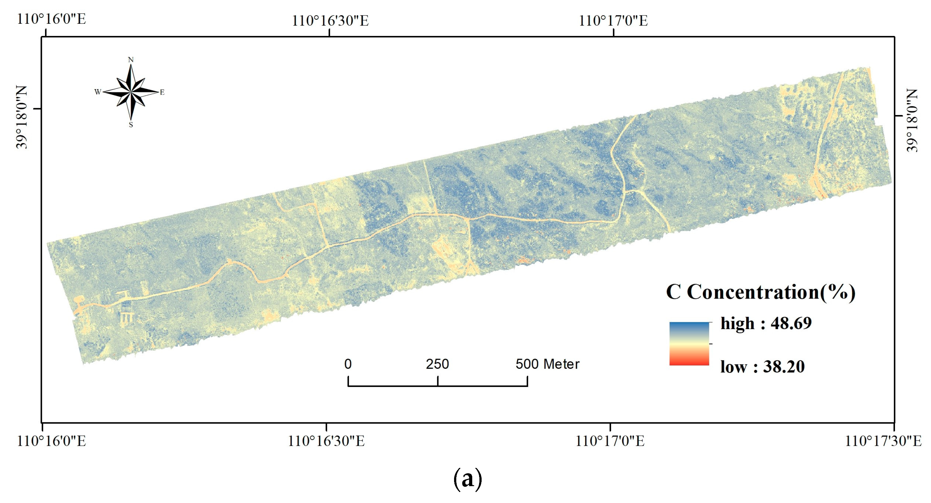
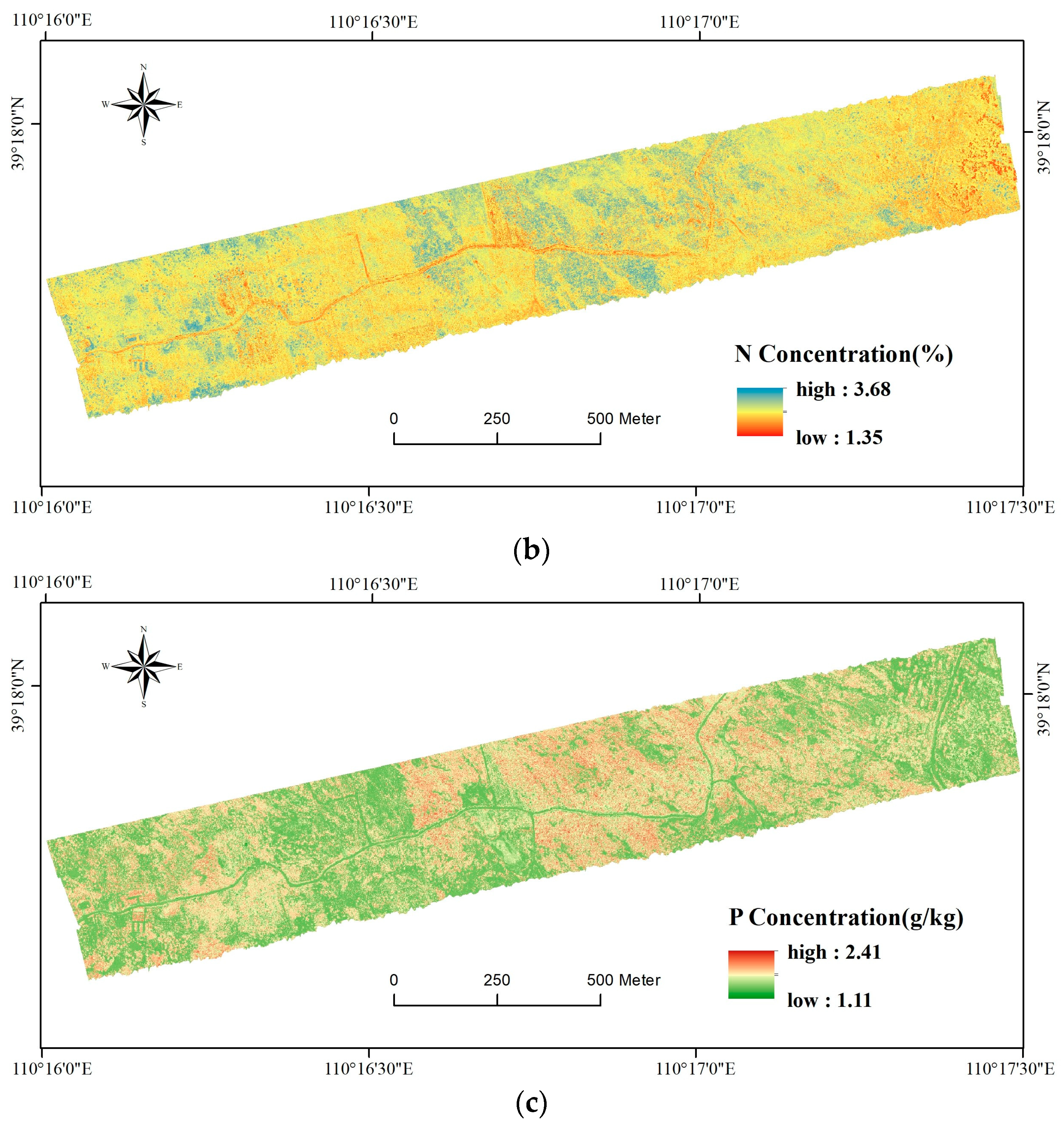
Foliar C, N, and P concentration maps were made to visualize the spatial distribution of these three nutrients. These maps were generated by applying random forest models to the images of the feature variables corresponding to the C, N, and P concentrations. Figure 8a–c illustrates the foliar C, N, and P concentrations in the study area, respectively. The spatial distribution of C, N, and P concentrations in each plant community was significantly different, which could effectively reflect the differences in C, N, and P concentrations among different plant communities.
The maximum C value, 48.70%, was observed in the Pinus sylvestris community, while the minimum, 38.20%, was found in the Herbaceous community. The average C concentration was 45.17%, with a median of 45.20%. The majority of C values were concentrated within the range of 42.20–48.00%. The high-value areas of C concentration were mainly found in the Sea buckthorn and Pinus sylvestris communities in the middle of the study area, and the low-value areas were mainly found in the Populus spp. and Herbaceous communities in the study area.
The maximum N value, 3.69%, was observed in the Caragana spp. community, while the minimum value, 1.35%, was found in the Herbaceous community. The average N concentration was 2.56%, with a median of 2.54%. The majority of values were concentrated within the range of 1.50–3.50%. The high-value areas of N concentration were mainly found in the Sea buckthorn community in the middle of the study area and scattered Populus spp. and Caragana spp. communities, while the low-value areas were mainly found in the Pinus sylvestris community near the main road and the Populus spp. community in the east.
The maximum P value, 2.42 g/kg, was observed in the Artemisia oleifera community, while the minimum value, 1.12 g/kg, was found in the Herbaceous community. The average P concentration was 1.65 g/kg, with a median of 1.63 g/kg. The majority of values were concentrated within the range of 1.30–2.20 g/kg. The high-value area of P concentration was mainly found in the Artemisia oleifera community in the middle of the study area, and the low-value areas were mainly found in the Pinus sylvestris, Populus spp., and Herbaceous communities in the study area.

4. Discussion

4.1. The Role of Features in the Model

Table 6 presents the hyperspectral and LiDAR features involved in constructing the models to measure the foliar C, N, and P concentrations. A total of 32 features were used in estimating both the C and N concentrations, including nine hyperspectral features and 23 LiDAR features for C along with 14 hyperspectral features and 18 LiDAR features for N. In the case of the P concentration estimation, 16 features were considered, consisting of 12 hyperspectral features and four LiDAR features.
For C, red-edge bands, height variables, and vegetation structure parameters were identified as comparatively important. For N, textural features, height percentiles of 40–95%, and vegetation structure parameters were deemed significant. As for P, spectral features, a height percentile of 80%, and a 1 m foliage height diversity were considered crucial. Among these, the 80% height percentile, height standard deviation, height variance, and 1 m leaf height diversity were identified as common features contributing to the construction of C, N, and P concentration estimation models, indicating their importance in estimating C, N, and P concentrations. Additionally, during the construction of the C concentration estimation model, the incorporation of LiDAR features significantly enhanced the predictive accuracy, suggesting that the C concentration is sensitive to plant height and can differentiate plant communities based on height. However, when constructing the N and P concentration estimation models, the inclusion of LiDAR features did not notably improve predictive accuracy, indicating that the sensitivity of N and P concentrations to plant height is limited; in addition, enhancing the accuracy of the N and P estimates did not rely heavily on the LiDAR features.

4.2. Implications of the Foliar C, N, and P Map

Considering the fact that the restoration of vegetation on degraded land is often limited by nutrient deficiency, C, N, and P maps can be used to examine nutrient limitation and storage in an area, so as to provide information supporting the post-restoration management of vegetation.
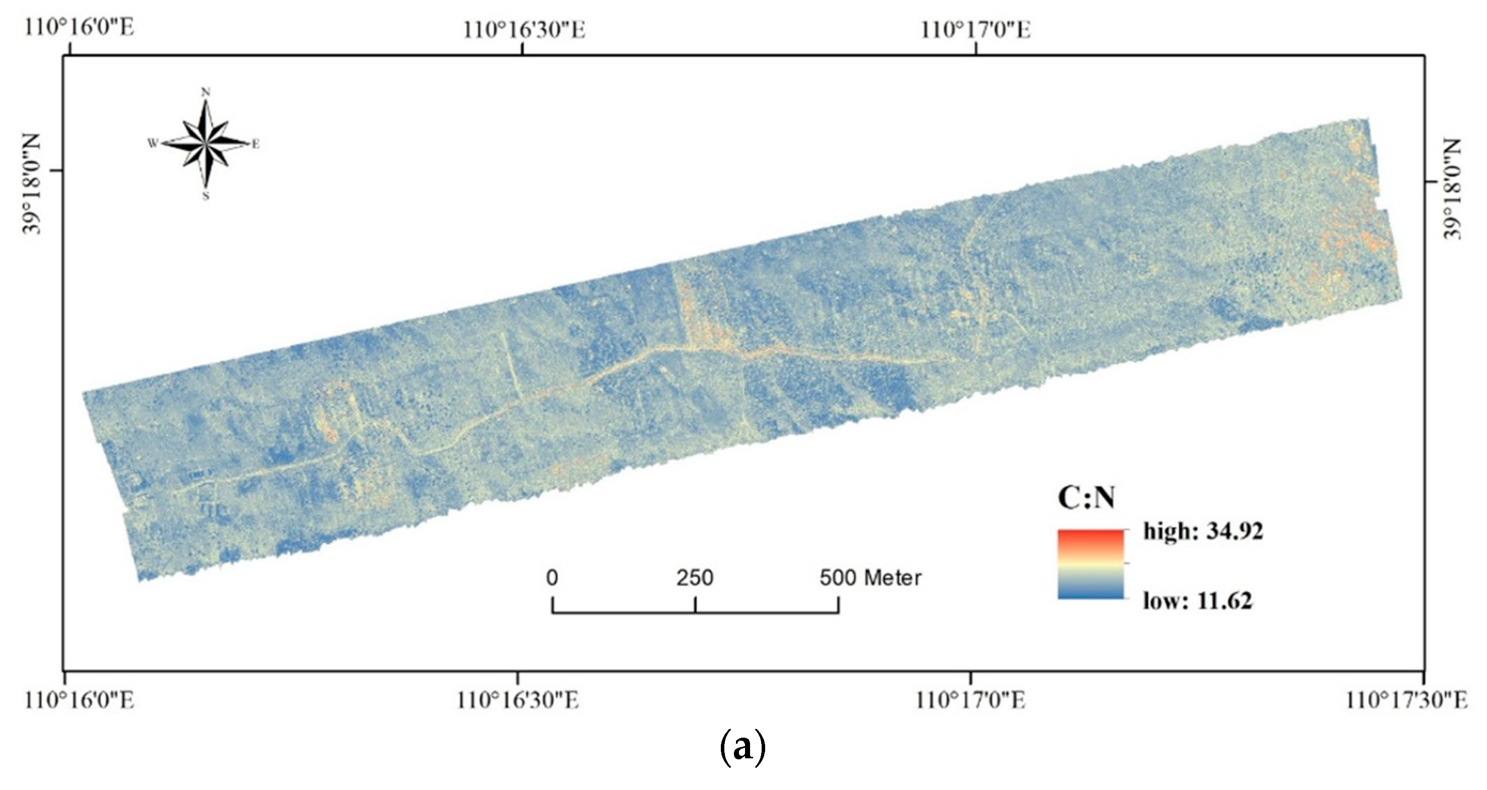
The C:N ratio reflects the vegetation’s ability to assimilate carbon (C) in relation to nitrogen (N) and its efficiency in utilizing nitrogen; this ratio also indicates the carbon sequestration capacity of the plant [72]. A high C:N ratio implies a relatively higher content of C and a lower content of N in the leaves. This may occur in environments with limited N supply, or when plants grow under conditions rich in C but deficient in N. Plants with a high C:N ratio exhibit high N use efficiency but grow slowly because they require more time to acquire sufficient N to support growth [73]. However, a low C:N ratio signifies a relatively low C content and a higher N content in the leaves. This typically indicates that the studied plants have an ample N supply, possibly due to being in an N-rich environment or receiving N fertilizer. Plants with a low C:N ratio have rapid decomposition traits and faster growth, with a relatively lower demand for C [73]. Plants with a moderate C:N ratio have a balanced content of C and N in their leaves. This usually suggests that plants are in a relatively balanced state in terms of C and N supply, are capable of adapting to various environmental conditions, and thrive under suitable conditions.
In the present study, the C:N ratios were calculated (Figure 9a). This figure shows that the Pinus sylvestris and Populus spp. communities had higher C:N ratios. This suggests that Pinus sylvestris and Populus spp. have relatively high N use efficiencies and stronger C sequestration capabilities, whereas Sea buckthorn, Artemisia oleifera, Amorpha fruticosa, and Caragana spp. have lower N use efficiencies and weaker carbon sequestration capabilities. The C:N ratios for the Salix spp. and Herbaceous plant communities were relatively balanced.
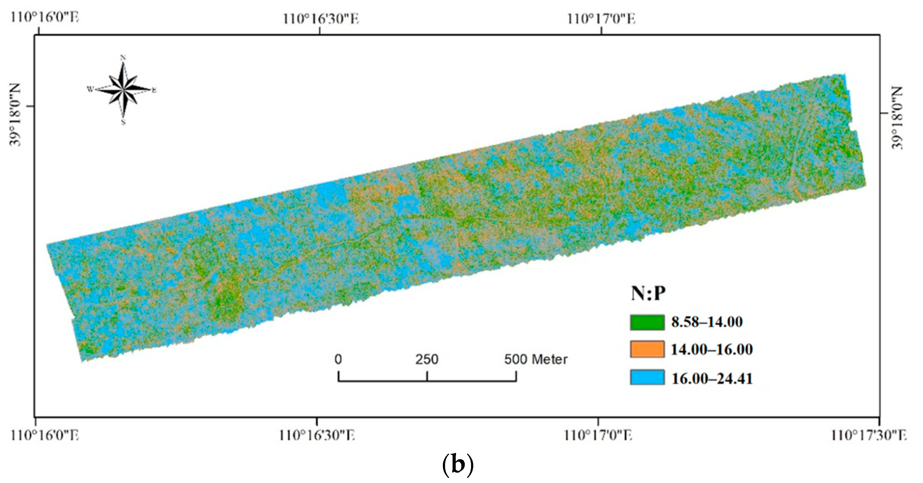
The N:P ratio reflects the availability of N and P in plants; the availability of N and P is a critical factor that can limit plant growth [74]. Therefore, analyzing the N:P ratio in plants can provide insights into the growth and nutrient limitations of plants. Typically, when the N:P ratio is between 14 and 16, plants are not limited by N or P or are co-limited by both. In contrast, when the N:P ratio is less than 14, plants are primarily limited by N, while when the N:P ratio is greater than 16, plants are mainly limited by P [75]. The N:P ratios for different plant canopies in the study area were generated from the N and P concentration maps (Figure 9b).
The blue region (46.62%) in Figure 9b primarily represents communities of Amorpha fruticosa, Sea buckthorn, and Caragana spp., with an N:P ratio greater than 16, indicating that these three plant communities were limited by P. The green region (20.06%) in the same figure mainly represents Pinus sylvestris, Artemisia oleifera, and Salix spp. communities, with an N:P ratio of less than 14, indicating that these three plant communities were limited by N. The orange region (30.32%) in that figure mainly represents Populus spp. and herbaceous communities, with an N:P ratio between 14 and 16, suggesting that these two plant communities may either not have been limited by N or P or they may have been co-limited by both.

4.3. Limitations and Future Work

This study has some limitations that need to be noted. First, the plant communities in the study area are mixed. Although LiDAR provides high accuracy, the richness of plant community types results in lower estimation accuracy when compared with conditions in communities with vegetation types composed of a single species such as wheat or corn [75,76]. Second, the limited spectral bands (398–1002 nm) in the hyperspectral data allow for only a partial inversion of C, N, and P concentrations, because sensitivity to these elements is lacking in certain bands (1000–2000 nm). Third, seasonal or monthly variations may affect the effectiveness of the developed approach. We suggest assessing the C, N, and P concentrations during the maturity period of vegetation growth. Moreover, the C, N, and P concentrations of different vegetation types should be conducted in the same observing time.
The developed approach is more suitable for semi-arid regions with less diverse vegetation. It can also be used in farmland, plantations, and natural forests to quickly assess foliar C, N, and P concentrations for fertilization management and ecosystem health assessment. For implementing the developed approach, the recommended procedures include, first, acquiring LiDAR and hyperspectral data by UAV, extracting the sensitive features using LiDAR 360 V6.0 software and ENVI 5.0 software, as shown in Table 6, training random forest models to generate maps of C, N, and P concentrations, and then validating the results. If the accuracy cannot be accepted, change the sensitive features and re-train the models, and, if accepted, the maps could be applied to show the status of foliar C, N, and P.
The technology employed in this study demonstrates significant potential, offering a synergistic approach for estimating foliar C, N, and P concentrations in plant communities and revealing their responses to ecological changes. Moreover, the monitoring results can be applied to ecological restoration management, ecosystem health assessment, and plant stress identification. The research shows substantial spatial heterogeneity, significantly reducing estimation accuracy, particularly in forests restored by humans that are often under C, N, and P limitations. The maps of C, N, and P could be used to explain the driving factors, such as soil, terrain, and vegetation, of restoration success. Considering that plant community types have a significant impact on LiDAR and hyperspectral features, in the future, it can be considered to classify mixed plant communities first, and then establish estimation models for C, N, and P concentration for each plant community type separately, reducing inter-class differences in data and achieving the goal of improving evaluation accuracy. In addition, this study only used shallow features from remote sensing images, such as plant height and vegetation index information. In the future, deep network models can be used to extract deep features, such as abstract semantic information from remotely sensed images and LiDAR point cloud data, to improve evaluation accuracy and efficiency. Expanding monitoring capabilities using satellite data to acquire C, N, and P information for ecological assessments or vegetation health monitoring is crucial for overcoming the limitations of traditional monitoring based on vegetation indices such as coverage and greenness.

5. Conclusions

This study used LiDAR and hyperspectral data to extract spectral features, textural features, vegetation indices, height features, and vegetation structural parameters for eight dominant plant communities in the Shendong Mining Area in China. Three models, namely, causal bands, multiple linear regression, and random forest models, were developed and tested in an ecological restoration area in northern China.
The key findings and conclusions of this research suggest that LiDAR and hyperspectral data can be used to effectively monitor the C, N, and P concentrations in a mixed plant community zone within an ecological restoration area. The random forest model demonstrated the best performance, with the optimal feature combination being hyperspectral + LiDAR data. This study revealed that C, N, and P concentrations effectively reflect differences among various regions and communities, indicating the stress levels on plants often caused by a lack of these elements. This approach offers a rapid and cost-effective means of acquiring related data, providing valuable information for the management and successful assessment of an ecological restoration area.
Based on the experience of this study, it is necessary to utilize hyperspectral data with a broader range of bands and perform classification for plant communities in this type of study. An extended spectral range can provide richer information for analyzing the spatial heterogeneity of foliar C, N, and P concentrations and their stress on vegetation growth after restoration. Plant classification may reduce the spatial and spectral uncertainties introduced by plant community heterogeneity, offering the potential to enhance the accuracy of predicting plant C, N, and P concentrations. Using this information for the analysis of C, N, and P limitations and ecosystem health assessment will contribute to a more precise understanding of ecosystem restoration.

Author Contributions

Conceptualization, experiment design, investigation, and writing, Y.Y.; methodology, validation, formal analysis, and software, J.D., J.T. and J.Z.; funding acquisition and resources, S.L.; supervision, and project administration, S.Z. and F.C. All authors have read and agreed to the published version of the manuscript.

Funding

This work was supported by the National Key Research and Development Program of China (2023YFF1306005) and the National Natural Science Foundation of China (52394193).

Data Availability Statement

The data presented in this study are available on request from the corresponding author.

Acknowledgments

We thank Guoneng Shendong Coal Group Co., Ltd. for the supporting of the fieldwork.

Conflicts of Interest

The authors declare no conflicts of interest.

References

  1. Sun, X.; Yuan, L.; Liu, M.; Liang, S.; Li, D.; Liu, L. Quantitative estimation for the impact of mining activities on vegetation phenology and identifying its controlling factors from Sentinel-2 time series. Int. J. Appl. Earth Obs. Geoinf. 2022, 111, 102814. [Google Scholar] [CrossRef]
  2. Chugh, Y.P.; Schladweiler, B.K.; Skilbred, C. Sustainable and responsible mining through sound mine closure. Int. J. Coal Sci. Technol. 2023, 10, 14. [Google Scholar] [CrossRef]
  3. Fischer, J.; Riechers, M.; Loos, J.; Martin-Lopez, B.; Temperton, V.M. Making the UN Decade on ecosystem restoration a social-ecological endeavour. Trends Ecol. Evol. 2020, 36, 20–28. [Google Scholar] [CrossRef] [PubMed]
  4. Krzyszowska Waitkus, A. Sustainable reclamation practices for a large surface coal mine in shortgrass prairie, semiarid environment (Wyoming, USA): Case study. Int. J. Coal Sci. Technol. 2022, 9, 32. [Google Scholar] [CrossRef]
  5. Banerjee, B.P.; Raval, S. Mapping sensitive vegetation communities in mining eco-space using UAV-LiDAR. Int. J. Coal Sci. Technol. 2022, 9, 40. [Google Scholar] [CrossRef]
  6. Zhang, Y.; Zhou, W. Remote sensing of vegetation fraction for monitoring reclamation dynamics: A case study in Pingshuo Mining area. In Proceedings of the 2016 IEEE International Geoscience and Remote Sensing Symposium (IGARSS), Beijing, China, 10–15 July 2016; pp. 5197–5200. [Google Scholar] [CrossRef]
  7. Ustin, S. Remote sensing of canopy chemistry. Proc. Natl. Acad. Sci. USA 2013, 110, 804–805. [Google Scholar] [CrossRef] [PubMed]
  8. Gastauer, M.; Silva, R.J.; Junior, C.F.C.; Ramos, S.J.; Filho, P.; Neto, A.; Siqueira, J.O. Mine land rehabilitation: Modern ecological approaches for more sustainable mining. J. Clean. Prod. 2018, 172, 1409–1422. [Google Scholar] [CrossRef]
  9. McGroddy, M.E.; Daufresne, T.; Hedin, L.O. Scaling of C: N: P stoichiometry in forests worldwide: Implications of terrestrial redfield-type ratios. Ecology 2004, 85, 2390–2401. [Google Scholar] [CrossRef]
  10. Han, W.; Fang, J.; Reich, P.B.; Ian Woodward, F.; Wang, Z. Biogeography and variability of eleven mineral elements in plant leaves across gradients of climate, soil and plant functional type in China. Ecol. Lett. 2011, 14, 788–796. [Google Scholar] [CrossRef]
  11. Xing, K.; Zhao, M.; Niinemets, U.; Niu, S.; Tian, J.; Jiang, Y.; Chen, H.; White, P.J.; Guo, D.; Ma, Z. Relationships between leaf carbon and macronutrients across woody species and forest ecosystems highlight how carbon is allocated to leaf structural function. Front. Plant Sci. 2021, 12, 674932. [Google Scholar] [CrossRef]
  12. Högberg, P.; Näsholm, T.; Franklin, O.; Högberg, M.N. Tamm review: On the nature of the nitrogen limitation to plant growth in Fennoscandian boreal forests. For. Ecol. Manag. 2017, 403, 161–185. [Google Scholar] [CrossRef]
  13. Urbina, I.; Sardans, J.; Grau, O.; Beierkuhnlein, C.; Jentsch, A.; Kreyling, J.; Peñuelas, J. Plant community composition affects the species biogeochemical niche. Ecosphere 2017, 8, e01801. [Google Scholar] [CrossRef]
  14. Güsewell, S. N:P ratios in terrestrial plants: Variation and functional significance. New Phytol. 2004, 164, 243–266. [Google Scholar] [CrossRef] [PubMed]
  15. Reich, P.B.; Oleksyn, J. Global patterns of plant leaf N and P in relation to temperature and latitude. Proc. Natl. Acad. Sci. USA 2004, 101, 11001–11006. [Google Scholar] [CrossRef] [PubMed]
  16. Xiong, J.; Yu, M.; Cheng, X.; Wang, C.; Zou, H. Effects of light and N-P supply ratios on growth and stoichiometric of Schimasuperba. Acta Ecol. Sin. 2021, 41, 2140–2150. [Google Scholar] [CrossRef]
  17. Avolio, M.L.; Koerner, S.E.; La Pierre, K.J.; Wilcox, K.R.; Wilson, G.W.T.; Smith, M.D.; Collins, S.L. Changes in plant community composition, not diversity, during a decade of nitrogen and phosphorus additions drive above-ground productivity in a tallgrass prairie. J. Ecol. 2014, 102, 1649–1660. [Google Scholar] [CrossRef]
  18. Stiles, W.A.V.; Rowe, E.C.; Dennis, P. Long-term nitrogen and phosphorus enrichment alters vegetation species composition and reduces carbon storage in upland soil. Sci. Total Environ. 2017, 593–594, 688–694. [Google Scholar] [CrossRef]
  19. McKenna, P.B.; Lechner, A.M.; Phinn, S.; Erskine, P.D. Remote sensing of mine site rehabilitation for ecological outcomes: A global systematic review. Remote Sens. 2020, 12, 3535. [Google Scholar] [CrossRef]
  20. Yang, Y.; Tang, J.; Zhang, Y.; Zhang, S.; Zhou, Y.; Hou, H.; Liu, R. Reforestation improves vegetation coverage and biomass, but not spatial structure, on semi-arid mine dumps. Ecol. Eng. 2022, 175, 106508. [Google Scholar] [CrossRef]
  21. Wang, J.; Wang, T.; Shi, T.; Wu, G.; Skidmore, A.K. A wavelet-based area parameter for indirectly estimating copper concentration in Carex Leaves from canopy reflectance. Remote Sens. 2015, 7, 15340–15360. [Google Scholar] [CrossRef]
  22. Dou, Z.; Cui, L.; Li, J.; Zhu, Y.; Gao, C.; Pan, X.; Lei, Y.; Zhang, M.; Zhao, X.; Li, W. Hyperspectral estimation of the chlorophyll content in short-term and long-term restorations of mangrove in Quanzhou Bay Estuary, China. Sustainability 2018, 10, 1127. [Google Scholar] [CrossRef]
  23. Liu, W.; Li, M.; Zhang, M.; Wang, D.; Guo, Z.; Long, S.; Yang, S.; Wang, H.; Li, W.; Hu, Y.; et al. Estimating leaf mercury content in Phragmites australis based on leaf hyperspectral reflectance. Ecosyst. Health Sustain. 2020, 6, 1726211. [Google Scholar] [CrossRef]
  24. Ren, H.; Zhao, Y.; Xiao, W.; Hu, H. A review of UAV monitoring in mining areas: Current status and future perspectives. Int. J. Coal Sci. Technol. 2019, 6, 320–333. [Google Scholar] [CrossRef]
  25. Nie, S.; Wang, C.; Zeng, H.; Xi, X.; Li, G. Above-ground biomass estimation using airborne discrete-return and full-waveform LiDAR data in a coniferous forest. Ecol. Indic. 2017, 78, 221–228. [Google Scholar] [CrossRef]
  26. Tang, J.; Liang, J.; Yang, Y.; Zhang, S.; Hou, H.; Zhu, X. Revealing the structure and composition of the restored vegetation cover in semi-arid mine dumps based on LiDAR and Hyperspectral Images. Remote Sens. 2022, 14, 978. [Google Scholar] [CrossRef]
  27. Ewald, M.; Aerts, R.; Lenoir, J.; Fassnacht, F.; Nicolas, M.; Skowronek, S.; Piat, J.; Honnay, O.; Garzón-López, C.; Feilhauer, H.; et al. LiDAR derived forest structure data improves predictions of canopy N and P concentrations from imaging spectroscopy. Remote Sens. Environ. 2018, 211, 13–25. [Google Scholar] [CrossRef]
  28. Zhang, Y.; Wang, T.; Guo, Y.; Skidmore, A.; Zhang, Z.; Tang, R.; Song, S.; Tang, Z. Estimating community-level plant functional traits in a species-rich alpine meadow using UAV image spectroscopy. Remote Sens. 2022, 14, 3399. [Google Scholar] [CrossRef]
  29. Bi, K.; Gao, S.; Niu, Z.; Zhang, C.; Huang, N. Estimating leaf chlorophyll and nitrogen contents using active hyperspectral LiDAR and partial least square regression method. J. Appl. Remote Sens. 2019, 13, 034513. [Google Scholar] [CrossRef]
  30. Yu, F.; Feng, S.; Yao, W.; Wang, D.; Xing, S.; Xu, T. BAS-ELM based UAV hyperspectral remote sensing inversion modeling of rice canopy nitrogen content. Int. J. Precis. Agric. Aviat. 2018, 1, 59–64. [Google Scholar] [CrossRef]
  31. Ye, X.; Abe, S.; Zhang, S. Estimation and mapping of nitrogen content in apple trees at leaf and canopy levels using hyperspectral imaging. Precis. Agric. 2020, 21, 198–225. [Google Scholar] [CrossRef]
  32. Cui, L.; Dou, Z.; Liu, Z.; Zuo, X.; Lei, Y.; Li, J.; Zhao, X.; Zhai, X.; Pan, X.; Li, W. Hyperspectral inversion of phragmites communis carbon, nitrogen, and phosphorus stoichiometry using three models. Remote Sens. 2020, 12, 1998. [Google Scholar] [CrossRef]
  33. Wang, Z.; Chen, J.; Zhang, J.; Tan, X.; Raza, M.A.; Ma, J.; Zhu, Y.; Yang, F.; Yang, W. Assessing canopy nitrogen and carbon content in maize by canopy spectral reflectance and uninformative variable elimination. Crop J. 2022, 10, 15. [Google Scholar] [CrossRef]
  34. Li, K.; Chen, Y.; Xu, Z.; Huang, X.; Hu, X.; Wang, X. Hyperspectral estimation method of chlorophyll content in Phyllostachys pubescens under pest stress. Spectrosc. Spectr. Anal. 2020, 40, 2578–2583. [Google Scholar] [CrossRef]
  35. Lohmann, P.; Koch, A.; Schaeffer, M. Approaches to the filtering of laser scanner data. Int. Arch. Photogramm. Remote Sens. 2000, 33, 540–547. [Google Scholar]
  36. Gitelson, A.A.; Keydan, G.P.; Merzlyak, M.N. Three-band model for noninvasive estimation of chlorophyll, carotenoids, and anthocyanin contents in higher plant leaves. Geophys. Res. Lett. 2006, 33, 431–433. [Google Scholar] [CrossRef]
  37. Maire, G.L.; Fran, O.C.; Dufrêne, E. Towards universal broad leaf chlorophyll indices using prospect simulated database and hyperspectral reflectance measurements. Remote Sens. Environ. 2004, 89, 1–28. [Google Scholar] [CrossRef]
  38. Richardson, A.J.; Wiegand, C.L. Distinguishing vegetation from soil background information. Photogramm. Eng. Remote Sens. 1977, 43, 100–120. [Google Scholar]
  39. Huete, A.; Justice, C.; Liu, H. Development of vegetation and soil indices for MODIS-EOS. Remote Sens. Environ. 1994, 49, 224–234. [Google Scholar] [CrossRef]
  40. Datt, B. A new reflectance index for remote sensing of chlorophyll content in higher plants: Tests using eucalyptus leaves. J. Plant Physiol. 1999, 154, 30–36. [Google Scholar] [CrossRef]
  41. Daughtry, C.S.T.; Walthall, C.L.; Kim, M.S.; De Colstoun, E.B.; McMurtrey Iii, J.E. Estimating corn leaf chlorophyll concentration from leaf and canopy re-flectance. Remote Sens. Environ. 2000, 74, 229–239. [Google Scholar] [CrossRef]
  42. Sims, D.A.; Gamon, J.A. Relationships between leaf pigment content and spectral reflectance across a wide range of species, leaf structures and developmental stages. Remote Sens. Environ. 2002, 81, 337–354. [Google Scholar] [CrossRef]
  43. Qi, J.; Chehbouni, A.; Huete, A.R.; Kerr, Y.H.; Sorooshian, S. A modified soil adjusted vegetation index. Remote Sens. Environ. 1994, 48, 119–126. [Google Scholar] [CrossRef]
  44. Driss, H.; John, R.M.; Elizabeth, P.; Pablo, J.Z.T.; Ian, B.S. Hyperspectral vegetation indices and novel algorithms for predicting green lai of crop canopies: Modeling and validation in the context of precision agriculture. Remote Sens. Environ. 2004, 10, 100–120. [Google Scholar] [CrossRef]
  45. Miller, J.R.; Hare, E.W.; Wu, J. Quantitative characterization of the vegetation red edge reflectance 1. An inverted-gaussian reflectance model. Int. J. Remote Sens. 1990, 11, 1755–1773. [Google Scholar] [CrossRef]
  46. Peuelas, J.; Gamon, J.A.; Fredeen, A.L.; Merino, J.; Field, C.B. Reflectance indices associated with physiological changes in nitrogen- and water-limited sunflower leaves. Remote Sens. Environ. 1994, 48, 135–146. [Google Scholar] [CrossRef]
  47. Rao, N.R.; Garg, P.K.; Ghosh, S.K.; Dadhwal, V.K. Estimation of leaf total chlorophyll and nitrogen concentrations using hyperspectral satellite imagery. J. Agric. Sci. 2008, 146, 65–75. [Google Scholar] [CrossRef]
  48. Thenot, F.; Méthy, M.; Winkel, T. The Photochemical Reflectance Index (PRI) as a water-stress index. Int. J. Remote Sens. 2002, 23, 5135–5139. [Google Scholar] [CrossRef]
  49. Blackburn, G.A. Spectral Indices for estimating photosynthetic pigment concentrations: A test using senescent tree leaves. Int. J. Remote Sens. 1998, 19, 657–675. [Google Scholar] [CrossRef]
  50. Metternicht, G. Vegetation indices derived from high-resolution airborne videography for precision crop management. Int. J. Remote Sens. 2003, 24, 2855–2877. [Google Scholar] [CrossRef]
  51. Schlerf, M.; Atzberger, C.; Hill, J. Remote sensing of forest biophysical variables using HyMap imaging spectrometer data. Remote Sens. Environ. 2005, 95, 177–194. [Google Scholar] [CrossRef]
  52. Merton, R.; Huntington, J. Early simulation of the ARIES-1 satellite sensor for multi-temporal vegetation research derived from AVIRIS. In Proceedings of the Summaries of the Eight JPL Airborne Earth Science Workshop, Pasadena, CA, USA, 8–11 February 1999; JPL Publication: Pasadena, CA, USA, 1999; Volume 99, pp. 299–307. [Google Scholar]
  53. Maccioni, A.; Agati, G.; Mazzinghi, P. New vegetation indices for remote measurement of chlorophylls based on leaf directional reflectance spectra. J. Photochem. Photobiol. B Biol. 2001, 61, 52–61. [Google Scholar] [CrossRef] [PubMed]
  54. Buschman, C.; Nagel, E. In vivo spectroscopy and internal optics of leaves as a basis for remote sensing of vegetation. Int. J. Remote Sens. 1993, 14, 711–722. [Google Scholar] [CrossRef]
  55. Huete, R.A. A Soil-Adjusted Vegetation Index (SAVI). Remote Sens. Environ. 1988, 20, 100–120. [Google Scholar] [CrossRef]
  56. McKee, T.B.; Doesken, N.J.; Kliest, J. The relationship of drought frequency and duration to time scales. In Proceedings of the Eighth Conference on Applied Climatology, American Meteorological Society, Anaheim, CA, USA, 17–22 January 1993; pp. 179–184. [Google Scholar]
  57. Broge, N.H.; Leblanc, E. Comparing prediction power and stability of broadband and hyperspectral vegetation indices for estimation of green leaf area index and canopy Chlorophyll density. Remote Sens. Environ. 2001, 76, 156–172. [Google Scholar] [CrossRef]
  58. Gitelson, A.A.; Kaufman, Y.J.; Stark, R.; Rundquist, D. Novel algorithms for remote estimation of vegetation fraction. Remote Sens. Environ. 2002, 80, 76–87. [Google Scholar] [CrossRef]
  59. Zarco-Tejada, P.J.; Miller, J.R.; Noland, T.L.; Mohammed, G.H.; Sampson, P.H. Scaling-up and model inversion methods with narrowband optical indices for chlorophyll content estimation in closed forest canopies with hyperspectral data. IEEE Trans. Geosci. Remote Sens. 2001, 39, 1491–1507. [Google Scholar] [CrossRef]
  60. Penuelas, J.; Pinol, J.; Ogaya, R.; Filella, I. Estimation of plant water concentration by the reflectance Water Index WI (R900/R970). Int. J. Remote Sens. 1997, 18, 2869–2875. [Google Scholar] [CrossRef]
  61. Kursa, M.B.; Rudnicki, W.R. Feature selection with the Boruta package. J. Stat. Softw. 2010, 36, 11. [Google Scholar] [CrossRef]
  62. Porder, S.; Asner, G.P.; Vitousek, P.M. Ground-based and remotely sensed nutrient availability across a tropical landscape. Proc. Natl. Acad. USA 2005, 102, 10909–10912. [Google Scholar] [CrossRef]
  63. Kokaly, R.F.; Asner, G.P.; Ollinger, S.V.; Martin, M.E.; Wessman, C.A. Characterizing canopy biochemistry from imaging spectroscopy and its application to ecosystem studies. Remote Sens. Environ. 2009, 113 (Suppl. 1), S78–S91. [Google Scholar] [CrossRef]
  64. Curran, P.J. Remote sensing of foliar chemistry. Remote Sens. Environ. 1989, 30, 271–278. [Google Scholar] [CrossRef]
  65. Wang, J.; Shi, T.; Liu, H.; Wu, G. Successive projections algorithm-based three-band vegetation index for foliar phosphorus estimation. Ecol. Indic. 2016, 67, 12–20. [Google Scholar] [CrossRef]
  66. Berger, K.; Verrelst, J.; Féret, J.B.; Hank, T.; Wocher, M.; Mauser, W.; Camps-Valls, G. Retrieval of aboveground crop nitrogen content with a hybrid machine learning method. Int. J. Appl. Earth Obs. Geoinf. 2020, 92, 174. [Google Scholar] [CrossRef]
  67. Homolová, L.; Malenovský, Z.; Clevers, J.G.P.W.; García-Santos, G.; Schaepman, M.E. Review of optical-based remote sensing for plant trait mapping. Ecol. Complex. 2013, 15, 1–16. [Google Scholar] [CrossRef]
  68. Huber, S.; Kneubühler, M.; Psomas, A.; Itten, K.; Zimmermann, N.E. Estimating foliar biochemistry from hyperspectral data in mixed forest canopy. For. Ecol. Manag. 2008, 256, 491–501. [Google Scholar] [CrossRef]
  69. van Deventer, H.; Cho, M.A.; Mutanga, O.; Ramoelo, A. Capability of models to predict leaf N and P across four seasons for six sub-tropical forest evergreen trees. ISPRS J. Photogramm. Remote Sens. 2015, 101, 209–220. [Google Scholar] [CrossRef]
  70. Peng, Y.; Zhang, M.; Xu, Z.; Yang, T.; Su, Y.; Zhou, T.; Wang, H.; Wang, Y.; Lin, Y. Estimation of leaf nutrition status in degraded vegetation based on field survey and hyperspectral data. Sci. Rep. 2020, 10, 4361. [Google Scholar] [CrossRef] [PubMed]
  71. Loozen, Y.; Rebel, K.T.; de Jong, S.M.; Lu, M.; Ollinger, S.V.; Wassen, M.J.; Karssenberg, D. Mapping canopy nitrogen in European forests using remote sensing and environmental variables with the random forests method. Remote Sens. Environ. 2020, 247, 111933. [Google Scholar] [CrossRef]
  72. Zhang, J.; He, N.; Liu, C.; Xu, L.; Chen, Z.; Li, Y.; Wang, R.; Yu, G.; Sun, W.; Xiao, C.; et al. Variation and evolution of C:N ratio among different organs enable plants to adapt to N-limited environments. Glob. Change Biol. 2020, 26, 2534–2543. [Google Scholar] [CrossRef]
  73. Song, S.; Xiong, K.; Chi, Y. Ecological stoichiometric characteristics of plant–soil–microorganism of grassland ecosystems under different restoration modes in the karst desertification area. Agronomy 2023, 13, 2016. [Google Scholar] [CrossRef]
  74. Koerselman, W.; Meuleman, A. The vegetation N:P ratio: A new tool to detect the nature of nutrient limitation. J. Appl. Ecol. 1996, 33, 1441–1450. [Google Scholar] [CrossRef]
  75. Yang, X.; Yuan, Z.; Ye, Y.; Wang, D.; Hua, K.; Guo, Z. Winter wheat total nitrogen content estimation based on UAV hyperspectral remote sensing. Spectrosc. Spectr. Anal. 2022, 42, 3269–3274. [Google Scholar] [CrossRef]
  76. Lapaz Olveira, A.; Saínz Rozas, H.; Castro-Franco, M.; Carciochi, W.; Nieto, L.; Balzarini, M.; Ciampitti, I.; Reussi Calvo, N. Monitoring corn nitrogen concentration from radar (C-SAR), optical, and sensor satellite data fusion. Remote Sens. 2023, 15, 824. [Google Scholar] [CrossRef]
Figure 1. Geographical situation of the study area (a,b) in Shaanxi Province, north China; (c) orthophoto view of the study area.
Remotesensing 16 01624 g001
Figure 2. Foliar carbon (C), nitrogen (N), and phosphorus (P) concentrations of eight dominant plant communities in the study area.
Remotesensing 16 01624 g002
Figure 3. Technical roadmap for foliar C, N, and P concentrations mapping. Note: LiDAR, laser imaging, detection, and ranging; MAE, mean absolute error; RMSE, root mean squared error; R2, coefficient of determination.
Remotesensing 16 01624 g003
Figure 4. Selection results of the features of (a) C, (b) N, and (c) P. All features were ranked according to the Z score calculated by the Boruta algorithm. The red, yellow, and green box plots represent the Z scores for the rejected, tentative, and confirmed features, respectively. For C, red-edge bands, height variables, and vegetation structure parameters were identified as comparatively important. For N, textural features, height percentiles of 40–95%, and vegetation structure parameters were deemed significant. For P, spectral features, a height percentile of 80%, and 1 m foliage height diversity were considered crucial.
Remotesensing 16 01624 g004aRemotesensing 16 01624 g004b
Figure 5. Accuracy of estimation model using causal bands for (a) C, (b) N, and (c) P.
Remotesensing 16 01624 g005
Figure 6. Accuracy of estimation model of multiple linear regression for (a) C, (b) N, and (c) P.
Remotesensing 16 01624 g006
Figure 7. Accuracy of estimation model of random forest for (a) C, (b) N, and (c) P.
Remotesensing 16 01624 g007
Figure 8. Study site maps produced using the random forest model for foliar: (a) C, (b) N, and (c) P concentrations.
Remotesensing 16 01624 g008aRemotesensing 16 01624 g008b
Figure 9. Maps of the foliar (a) C:N and (b) N:P ratios in the study area.
Remotesensing 16 01624 g009aRemotesensing 16 01624 g009b
Table 1. Foliar carbon (C), nitrogen (N), and phosphorus (P) concentrations based on sample data.
MinMaxMeanStandard Deviation
C (%)34.4652.2845.802.36
N (%)1.094.062.620.87
P (g/kg)0.633.081.730.49
Table 2. Calculation formulas of texture features.
No.Texture FeatureFormula
1Mean i = 0 N 1 j = 0 N 1 i P ( i , j )
2Variance i = 0 N 1 j = 0 N 1 ( i u ) 2 P ( i , j )
3Entropy i = 0 N 1 j = 0 N 1 P ( i , j ) log P ( i , j )
4Data range P ( i , j ) max P ( i , j ) min
5Skewness 1 N i = 0 N 1 j = 0 N 1 P ( i , j ) u σ 3
Table 3. Calculation formulas of vegetation indices.
No.IndicesFormula
1CIgreen [36] ( R 780 / R 550 ) 1
2CIred_edge [36] ( R 780 / R 710 ) 1
3DD [37] ( R 750 R 722 ) / ( R 700 R 670 )
4DVI [38] R 800 R 670
5EVI [39] [ 0.5 × ( R 800 R 638 ) ] / ( R 800 + 2.5 × R 800 6.0 × R 472 + 7.5 )
6GM [36] R 750 / R 702
7GNDVI [36] ( R 780 R 552 ) / ( R 780 + R 552 )
8LCI [40] ( R 850 R 710 ) / ( R 850 + R 682 )
9MCARI [41] [ ( R 720 R 680 ) 0.2 × ( R 720 R 550 ) ] × ( R 720 / R 680 ) ]
10mND705 [42] ( R 750 R 705 ) / ( R 750 + R 705 2 × R 445 )
11MSAVI [43] 0.5 × ( 2 × R 800 + 1 ( 2 × R 800 + 1 ) 2 8 × ( R 800 R 680 ) )
12mSR705 [37] ( R 750 R 445 ) / ( R 705 R 445 )
13MTVI1 [44] 1.2 × [ 1.2 × ( R 802 R 550 ) 2.5 × ( R 670 R 550 ) ]
14NDI [36] ( R 834 R 662 ) / ( R 834 + R 662 )
15NDVI [45] ( R 450 R 680 ) / ( R 450 + R 680 )
16NPCI [46] ( R 450 R 680 ) / ( R 450 + R 680 )
17PBI [47] R 810 / R 562
18PRI [48] ( R 531 R 570 ) / ( R 531 + R 570 )
19PSNDa [49] ( R 802 R 682 ) / ( R 802 + R 682 )
20PSNDb [49] ( R 802 R 634 ) / ( R 802 + R 634 )
21PVR [50] ( R 550 R 650 ) / ( R 550 + R 650 )
22RVI [51] R 800 / R 670
23RVSI [52] ( R 714 R 752 ) / 2 R 733
24R680 [53]Reflectance at 680 nm
25R800 [54]Reflectance at 800 nm
26SAVI [55] ( R 800 R 670 ) / [ 1.5 × ( R 800 + R 670 + 0.5 ) ]
27SPI [56] ( R 802 R 450 ) / ( R 802 + R 682 )
28SRPI [46] R 430 / R 680
29TVI [57] 0.5 × [ 120 × ( R 750 R 550 ) 200 × ( R 670 R 550 ) ]
30VARI [58] ( R 730 R 662 ) / ( R 730 + R 662 )
31VOGa [59] R 742 / R 722
32VOG2 [59] ( R 742 R 746 ) / ( R 714 + R 722 )
33WI [60] R 900 / R 970
Note, R680 in the table indicates the spectral reflectance at 680 nm; other parameters are analogized. Chlorophyll index—green (CIgreen); chlorophyll index—red edge (CIred_edge); double difference index (DD); difference vegetation index (DVI); enhanced vegetation index (EVI); Gitelson and Merzlyak index (GM); green normalized difference vegetation index (GNDVI); land cover index (LCI); modified chlorophyll absorption in reflectance index (MCARI); modified normalized difference (mND705); modified simple ratio (mSR705); modified soil-adjusted vegetation index (MSAVI); modified triangular vegetation index (MTVI1); normalized vegetation index (NDI); normalized difference vegetation index (NDVI); normalized pigment chlorophyll index (NPCI); plant biochemical index (PBI); photochemical reflectance index (PRI); pigment specific normalized difference of chlorophyll a (PSNDa); pigment specific normalized difference of chlorophyll b (PSNDb); perpendicular vegetation reflectance (PVR); ratio vegetation index (RVI); red edge vegetation stress index (RVSI); the range of leaf reflectance at 680 nm (R680); the range of leaf reflectance at 800 nm (R800); soil-adjusted vegetation index (SAVI); standardized precipitation index (SPI); simple ratio pigment index (SRPI); triangle vegetation index (TVI); visual atmospheric resistant index (VARI); Vogelmann red edge index 1 (VOGa); Vogelmann red edge index 2 (VOG2); water index (WI).
Table 4. Variable symbols of laser imaging, detection, and ranging (LiDAR) features.
No.LiDAR FeaturesVariable Symbols
1Maximum heightHmax
2Minimum heightHmin
3Average heightHmean
4Height kurtosisHkurt
5MedianHmedian_z
6Height skewnessHskew
7Height standard deviationHstd
8Height varianceHvar
9Canopy relief ratioHcrr
10Canopy density metricsd0, d1, d2, d3, d4, d5, d6, d7, d8, d9
11Height percentileHP1st, HP5th, HP10th, HP20th, HP25th, HP30th, HP40th, HP50th, HP60th, HP70th, HP75th, HP80th, HP90th, HP95th, HP99th
12Canopy heightCHM
13Canopy coverCC
14Gap fractionGF
15Leaf area indexLAI
16Foliage height diversityFHD-1m, FHD-2m, FHD-3m
Note, that the calculation of the features above can be found in our previous research [26].
Table 5. Accuracy of the estimation models.
ModelFeature CombinationR2RMSEMAE
CCausal bands(970, 990 nm)0.075.163.64
Multiple linear regression modelHyperspectral features0.344.693.11
Hyperspectral + LiDAR0.422.242.13
Random forest modelHyperspectral features0.383.472.74
Hyperspectral + LiDAR0.561.191.00
NCausal bands(510, 700–750, 910 nm)0.200.920.60
Multiple linear regression modelHyperspectral features0.460.870.52
Hyperspectral + LiDAR0.480.850.48
Random forest modelHyperspectral features0.530.570.46
Hyperspectral + LiDAR0.530.570.46
PCausal bands(400–900 nm)0.320.520.45
Multiple linear regression modelHyperspectral features0.370.510.36
Hyperspectral + LiDAR0.390.500.36
Random forest modelHyperspectral features0.430.400.31
Hyperspectral + LiDAR0.440.400.31
Table 6. The hyperspectral and LiDAR features employed for estimating C, N, and P concentrations.
Hyperspectral FeaturesCNPLiDAR FeaturesCNP
R399 d6
R404 d8
R409 d9
R415 Hmax
R420 Hmean
R451 Hmedian_z
R462 HP1st
R473 HP10th
R483 HP20th
R504 HP25th
R510 HP30th
R515 HP40th
R758 HP50th
R763 HP60th
EVI HP70th
GNDVI HP75th
MTVI1 HP80th
NPCI HP90th
PVR HP95th
R680 HP99th
SRPI Hstd
WI Hvar
B1-Data Range CC
B1-Mean CHM
B1-Variance FHD-1m
B3-Data Range FHD-2m
B3-Variance FHD-3m
////GF
Disclaimer/Publisher’s Note: The statements, opinions and data contained in all publications are solely those of the individual author(s) and contributor(s) and not of MDPI and/or the editor(s). MDPI and/or the editor(s) disclaim responsibility for any injury to people or property resulting from any ideas, methods, instructions or products referred to in the content.