A Holistic View of Global Croplands and Their Water Use for Ensuring Global Food Security in the 21st Century through Advanced Remote Sensing and Non-remote Sensing Approaches

Thenkabail, Prasad S.; Hanjra, Munir A.; Dheeravath, Venkateswarlu; Gumma, Muralikrishna

doi:10.3390/rs2010211

Open AccessArticle

A Holistic View of Global Croplands and Their Water Use for Ensuring Global Food Security in the 21st Century through Advanced Remote Sensing and Non-remote Sensing Approaches

by

Prasad S. Thenkabail

^1,*,

Munir A. Hanjra

²,

Venkateswarlu Dheeravath

³ and

Muralikrishna Gumma

⁴

¹

Southwest Geographic Science Center, U.S. Geological Survey, Flagstaff, AZ 86001, USA

²

International Centre of Water for Food Security, Charles Stuart University, NSW 2678 Australia

³

United Nations Joint Logistic Center, World Food Program (WFP), Juba, South Sudan, SudanUnited Nations Joint Logistic Center, World Food Program (WFP), Juba, South Sudan, Sudan

⁴

International Water Management Institute, Hyderabad, India

^*

Author to whom correspondence should be addressed.

Remote Sens. 2010, 2(1), 211-261; https://doi.org/10.3390/rs2010211

Submission received: 6 November 2009 / Revised: 26 November 2009 / Accepted: 2 January 2010 / Published: 4 January 2010

(This article belongs to the Special Issue Global Croplands)

Download

Browse Figures

Versions Notes

Abstract

:

This paper presents an exhaustive review of global croplands and their water use, for the end of last millennium, mapped using remote sensing and non-remote sensing approaches by world’s leading researchers on the subject. A comparison at country scale of global cropland area estimated by these studies had a high R²-value of 0.89–0.94. The global cropland area estimates amongst different studies are quite close and range between 1.47–1.53 billion hectares. However, significant uncertainties exist in determining irrigated areas which, globally, consume nearly 80% of all human water use. The estimates show that the total water use by global croplands varies between 6,685 to 7,500 km³ yr⁻¹ and of this around 4,586 km³ yr⁻¹ is by rainfed croplands (green water use) and the rest by irrigated croplands (blue water use). Irrigated areas use about 2,099 km³ yr⁻¹ (1,180 km³ yr⁻¹ of blue water and the rest from rain that falls over irrigated croplands). However, 1.6 to 2.5 times the blue water required by irrigated croplands is actually withdrawn from reservoirs or pumping of ground water, suggesting an irrigation efficiency of only between 40–62 percent. The weaknesses, trends, and future directions to precisely estimate the global croplands are examined. Finally, the paper links global croplands and their water use to a paradigm for ensuring future food security.

Keywords:

croplands; remote sensing; water use; virtual water; food security; water productivity

Graphical Abstract

1. Introduction

Global change is putting unprecedented pressure on global croplands, vital for ensuring future food security for all. Declining per capita agricultural production requires immediate policy responses to safeguard food security amidst global climate change and economic turbulence. The precise estimation of global croplands and their precise location are critical scientific tools for any policy response [1,2,3] at a time when most indicators point to worsening food security situation [4,5,6]. For instance, world food stocks are fast dwindling [7], cropland areas have nearly stagnated, yield per unit area have plateaued [8], world population is increasing at nearly 100 million per year [9], croplands are being lost to biofuel production [10], salinization [11], and urbanization [12,13], and nutritional transition is raising the calorie intake swiftly in emerging markets due to economic change [14]. Already, recent global trends suggest that grain production increases are becoming more difficult to achieve as a result of increasing population, and as the competition for water intensifies between agriculture, cities and the environment [15]. There is a need to reduce the environmental footprint of food production. Declining per capita agricultural production and warming oceans are emerging threats to global and regional food security [16]. The drop in grain production in the Northern China Plain, which produces over half of China’s wheat and a third of corn, from its peak of 392 million tons in 1998 to 338 million tons in 2003 (a drop equivalent to Canada’s entire harvest) has been attributed to the declining watertables and resulting loss of irrigated areas [17]. This is significant, since just a 3% drop in China’s cereal production will claim 10% of the world export market and can potentially jeopardize global food security [18]. Also, in China’s Yangtze Delta, for example, rice paddy areas have decreased by a dramatic 22% over the last six decades, while an increase has been seen for urban areas (8%) and aquaculture (14%) [19]. Global wheat stocks reached historic lows this decade and wheat prices increased by about 30% in 2008 [20], resulting in further structural changes in global grain markets, and increased rice prices in recent years have also endangered food security [14,21]. The global food outlook and price trends remains pessimistic and appear set to continue [22] over the medium term to 2015 [7], a year when the progress towards eradicating world hunger and other Millennium Development Goals will be judged by the United Nations [23]. Food commodity speculation and derivatives are a new cause of malnutrition [24]. Continuous food crisis will be new global norm unless international agricultural research and investment efforts are directed to find long term solution to the world food security crisis [25].

Increasing cropland areas for food security may not be feasible, due to potential negative environmental impacts of the area expansion [26]. For instance, land use land cover (LULC) changes, specifically deforestation for crop production, are shown to have a stronger influence on ecosystem carbon budgets than the projected climate change scenarios [27]. Cropland soils hold the key to terrestrial carbon (C) sequestration as well [28,29], accounting for 0.5–0.7 GtC yr⁻¹ in mid-century [30]. The contribution from agricultural no-till soils by itself be about 40% by mid-century [30]. At current levels, agricultural croplands account for 50% of methane (CH₄) and 60% of nitrous oxide emissions [31]. Irrigated rice paddies are a major source of atmospheric CH₄ [32,33].

Above all, croplands are also water guzzlers [34], taking anywhere between 60% and 90% of all human water use. With increasing urbanization, industrialization, and other demands on water, there is increasing pressure to reduce agricultural water use. Conversion from natural vegetation to irrigated cropland also means greater water use. When large tracts of a river basin are converted from natural vegetation to irrigated croplands, they will result in a substantial reduction in the volume of water in streams. Recent research in Brazil using Landsat data showed that the regional mean ET for irrigated crops was 3.6 mmd⁻¹, being higher by an order of magnitude than for natural vegetation (1.4 mmd⁻¹) [35].

The above factors imply that there is a need to produce more food from existing or even reduced (a) areas of croplands (more crop per unit area); and (b) quantum of water (more crop per drop). More crop per unit area (crop productivity) along with crop intensification led to the Green Revolution during 1960–2000, that helped build food barriers against episodes of hunger [36] and lifted millions out of malnutrition and poverty [37]. But, the Green Revolution has more or less stagnated lately, and declining yield gains are failing to keep up with population growth. More crop per drop (water productivity) is a concept that has yet to take off, but holds much promise amid caution [38]. In order to produce more food from existing croplands and water resources, precise maps and data on croplands and their water use are needed.

Thereby, emerging strategies for feeding the growing population in spite of the stagnated and even decreasing cropland areas will be to [1]:

(A): grow less water consuming crops (e.g., more wheat and less rice);
(B): increase water productivity through better water management and increasing irrigation efficiency;
(C): educate people to eat less water consuming food (e.g., more vegetables and grains compared to meat; more local and seasonal foods); and
(C): emphasize rainfed crop productivity to reduce stress on water-intensive irrigated croplands.

For planning these strategies and related incentive measures, we need to know the precise spatial location of agricultural crops, their water source (e.g., irrigation and/or rainfed), land use changes (e.g., biofuel vs. food crops), and water use patterns (e.g., water productivity maps). Such an effort will help agricultural policy makers and managers to plan and implement strategic goals of food security through renewed investments in agriculture, education and markets [25,37] and direct involvement of local governments and farmers to enhance the future food security [39 this issue].

Given the above background, the overarching goal of this paper is to produce a holistic review of the current state-of-art on information pertaining to global croplands and their water use with the aim to work towards a strategy for a food secure world. The main purpose of the paper is to identify the weaknesses and trends in existing methods and approaches and provide future directions to precisely estimate the global croplands. More precise estimates of global croplands are essential for future food security.

2. Global Croplands

Global croplands include irrigated and rainfed lands, but do not include pasture and rangelands. Cropland mapping at the global level [40,41,42] has become feasible by integrating agricultural statistics and census data from the national systems with spatial mapping technologies involving geographic information systems (GIS). More recently, availability of advanced remote sensing data along with secondary data and recent advances in data access, quality, processing, and delivery have made remote sensing based cropland estimates at the global level possible [1,2]. The specific remote sensing advances enabling global cropland mapping and generation of their statistics include factors such as: (a) free access to well calibrated and guaranteed data such as Landsat and (Moderate Resolution Imaging Spectroradiometer) MODIS; (b) frequent temporal coverage of data such as MODIS backed by high resolution Landsat data; (c) free access to high quality secondary data such as long-term precipitation, evapotranspiration, surface temperature, soils, and Global Digital Elevation Model (GDEM); (d) global coverage of the data; (e) web-access to data and faster download; (f) advances in computer technology; and (g) advances in processing. Prior to this, irrigated and rainfed cropland areas were estimated, at large scale, in global land use classifications [43,44,45,46,47] derived from remote sensing, which usually focused on other objectives, such as LULC for forestry, rangelands and rain-fed croplands. Most remote sensing work at regional level produced LULC maps and not specific thematic maps like croplands. The Global Land Cover Map produced by USGS [43] using Advanced Very High-Resolution Radiometer (AVHRR) 1-km data had four irrigated classes: irrigated grassland, rice paddy and field, hot irrigated cropland, and cool irrigated cropland.

Currently, there are four main global cropland maps produced in recent times for the end of the last millennium. These are:

Thenkabail et al. [1]—Figure 1;
Ramankutty and Foley [48] —Figure 2;
Goldewijk et al. [42]—Figure 3; and
Portmann et al. [41] and Siebert and Döll [49]—Figure 4.

Globally, cropland areas increased from 265 Mha in 1700 to 1,471 Mha in 1990, while the area of pasture increased more than six fold from 524 to 3,451 Mha [50]. By these estimates, agriculture and pasture cover about 33% of the world’s land area. Foley et al. [51] and Ramankutty and Foley [48] estimate cropland and pasture to be nearly 40% of the world's terrestrial surface (148,940,000 Km²). The first remote sensing based global cropland estimate [1,2] for the nominal year 2000 showed global croplands as 1.53 billion hectares (Figure 1, Table 1). However, in all these studies, there is substantial scope for improvement in the precise spatial location of croplands, their characteristics (e.g., cropping intensity, crop calendar, type of crop grown), and their area estimates.

The four major global cropland studies [1,2,40,41,42,49] estimated total cropland areas between 1.30 to 1.53 Bha. Ramankutty et al. [40] (Figure 2) and Goldewijk [42] (Figure 3) do not differentiate between irrigated and rainfed cropland areas whereas Thenkabail et al. [1,2] (Figure 1) and Portsmann et al. [41] (Figure 4) and Siebert and Döll [49] (Figure 4) provide distinct irrigated and rainfed cropland statistics. A country-by-country comparison between cropland area estimates of different studies showed very high correlations. As shown in Figure 5a and Figure 5b Ramankutty et al. [40] used a combination of agricultural statistics and remote sensing to determine cropland areas of 197 countries that were highly correlated (R² value of 0.89) with the remote sensing based estimates of Thenkabail et al. [1,2]. Similarly, even though Portsmann et al. [41] and Siebert and Döll [49] used non-remote sensing approaches involving agricultural statistics and GIS and Thenkabail et al. [1,2] used remote sensing approaches, a comparison of cropland areas derived using two products for the 197 countries showed remarkable correlation with R² value of 0.94 (Figure 5b). Nevertheless, various coarse resolution cropland area mappings have two highly significant differences: (A) Precise spatial location of these cropland areas; and (B) Estimates of irrigated areas versus rainfed areas.

Both of these are crucial for water use assessments and practical applications of the data including food security planning. In addition to cropland maps and statistics, there are two premier global irrigated area maps and statistics. These are:

5.: Thenkabail et al. [1,2]—Figure 1; and
6.: Siebert et al. [52]—Figure 4.

These two premier products on irrigated areas are also referred as: (1) The International Water Management Institute’s (IWMI) global irrigated area map (GIAM), which is based on coarse resolution remote sensing [1,2,53,54]; and (2) Food and Agricultural Organization of the United Nations and the University of Frankfurt (FAO/UF’s) global map of irrigated areas (GMIA), which is based on national statistics [52] (Figure 4, Table 1). The Siebert et al. [52] study provides estimates of global area “equipped” for irrigation (but not necessarily irrigated) as 278.8 Mha, which is about 19% of the total croplands (1.5 Bha) around the year 2000. The Thenkabail et al. [1,2] study provides two types of areas: (a) total area available for irrigation (TAAI), which does not consider cropping intensity, and (b) annualized irrigated areas (AIA) which considers the intensity. The TAAI, which is equivalent to FAO/UF’s “areas equipped for irrigation” definition, was 399 Mha (Figure 1). This is nearly 120 Mha higher than FAO/UF estimates. The main differences occur in China and India. The AIA, which has no equivalent in FAO/UF statistics, was 467 Mha.

The importance of irrigation to global food security is highlighted in a recent study by Siebert and Döll [49] who show that without irrigation there would be decrease in production of various foods including dates (60%), rice (39%), cotton (38%), citrus (32%) and sugarcane (31%) from their current levels. Globally, without irrigation cereal production in irrigated areas will decrease by massive 43%, with overall cereal production, from irrigated and rainfed croplands, decreasing by 20%. As the world’s population grew from 2.2 billion in 1950 to 6.1 billion in 2001, irrigation played a major role in tripling of the world grain harvest from 640 million tons to 1,855 million tons [17]. Irrigated agriculture currently meets about 40% of global food needs from just 20% of the area that is irrigated. Khan et al. [55] studied irrigation systems in Australia, China, and Pakistan to show that none of them were sustainable in the current operational conditions as a result of soil salinity [56], lack of adequate water resources, groundwater mismanagement, and the mismatch between water policy and environmental policy for agricultural sustainability [11]. In contrast, rainfed croplands meet 60% of the food and nutritional needs of the world’s population from 80% of the global croplands. Irrigated lands are at least twice more productive than rainfed croplands though the latter are considered more environmentally friendly, and remain important to the food security of the marginal or subsistence farmers in many developing countries [1,2,57].

Figure 1. Global cropland map by Thenkabail et al. [1,2]. This includes irrigated and rainfed areas of the world as well as permanent crops. The product is derived using remotely sensed data. Total area of croplands is 1.53 billion hectares of which 399 million hectares is total area available for irrigation (without considering cropping intensity) and 467 million hectares is annualized irrigated areas (considering cropping intensity). The product is derived using 1–10 km base data. The output is given in nominal 1–km resolution. Also see: http://www.iwmigiam.org.

Figure 2. Global cropland map by Ramankutty et al. [40] and Ramankutty and Foley [48]. This includes irrigated and rainfed areas of the world as well as permanent crops. Total area of croplands is 1.47 billion hectares. The product is derived using national agricultural census data and remote sensing derived land use. The output is given in nominal 5-min (0.083333 decimal degrees) resolution.

Figure 3. Global irrigated cropland area map by Goldewijk et al. [42]. This includes irrigated and rainfed areas of the world as well as permanent crops. Total area of croplands is 1.47 billion hectares. The product is derived using national agricultural census data and remote sensing land use. The output is given in nominal 5-min (0.083333 decimal degrees) resolution.

Figure 4. Global irrigated cropland area map [52]. This includes only areas “equipped” for irrigation in the world. Total area of irrigated croplands is 278 Mha. The product is derived using the national agricultural census data and GIS. The output is given in nominal 5-min (0.083333 decimal degrees) resolution.

3. Uncertainties in Cropland Area Estimates

Uncertainties in cropland estimates (Table 1) are well established [1,58]. The greatest difficulty and differences in global cropland estimates is in differentiating between rainfed croplands versus irrigated croplands. This is also the most crucial difference because water use assessments and food production estimates depend heavily on whether an area is irrigated or rainfed.

A country-wise assessment of global irrigated areas using a remote sensing approach [1,2] (irrigated areas in Figure 1) and a non-remote sensing approach [52] (Figure 4) showed a clear trend with high correlations (R² value between 0.89 and 0.94; Figure 5a and Figure 5b). However, there are highly significant differences for China and India—the two countries with nearly 60% of all annualized irrigated areas of the world.

Figure 5a. Cropland areas per year (annualized) compared for 197 countries [1,2, versus 40]. Cropland areas include irrigated and rainfed crops as well as permanent crops. Ramankutty et al. [40] used national agricultural statistics fused with remote sensing data whereas Thenkabail et al. [1,2] used advanced remote sensing approaches. There is remarkably high correlation (R² value of 0.89) for the 1:1 line for comparison, at countries scale, of cropland areas between the two approaches. However, large differences in areas for some countries are clear. Reasons for the differences are discussed in the paper.

Figure 5b. Cropland areas per year (annualized) for 197 countries [1,2, versus 41,49]. Cropland areas include irrigated plus rainfed crops per year as well as permanent crops. Portmann et al. [41] and Siebert and Döll [49] use national agricultural statistics and geographic information systems (GIS) whereas Thenkabail et al. [1,2] use remote sensing approaches. There is remarkably high correlation (R² value of 0.94) for the 1:1 line for a country-by-country comparison of cropland areas between the two approaches. However, large differences in areas for some countries are clear. Reasons for differences are discussed in the paper.

The main causes of differences in areas reported in various studies can be attributed to [3,47,59], but not limited to: (a) reluctance on part of states to furnish irrigated census area data in view of their vested interests in sharing of water; (b) reporting of large volumes of census data with inadequate statistical analysis; (c) subjectivity involved in observation-based data collection process; (d) inadequate accounting of irrigated areas, especially minor irrigation from groundwater, in the national statistics; (e) definition issues involved in mapping using remote sensing as well as national statistics; (f) difficulties in arriving at precise estimates of area fractions (AFs) using remote sensing; (g) difficulties in separating irrigated from rainfed croplands; and (h) imagery resolution in remote sensing.

Even when cropland area estimates match reasonably well [1,40,41,42] (Figure 1, Figure 2 and Figure 3, Table 1) (Figure 6a–Figure 6b) there are serious mismatches in their exact spatial location and distribution of crops. One of the biggest causes of uncertainty is inadequate accounting of minor irrigation (from groundwater, small reservoirs, and tanks). In India, for example, the number of tube-wells increased from a meager 100,000 in early 1960s to about 26 million by the year 2000 [60]. However, the irrigated area maps and statistics on groundwater irrigation are sketchy and/or missing [61]. Indeed, overwhelming evidence [59,60,61,62] shows that much of the potential is already exploited but these do not show up as irrigated area maps [63]. Massive exploitation of surface water from minor reservoirs and/or tanks is a missing link in many irrigated area statistics. Wide discrepancies exist in tank irrigation area, even in the States where tanks have historically been an important source of irrigation [64]. Often groundwater and small reservoir irrigation are mapped as rainfed croplands. Similarly, definition issue is another main factor for differences in the areas. The “supplemental” irrigated areas are croplands that can sustain a crop only with substantial irrigation, but they are often labeled as rainfed.

China is important to world food security [18]. Yet, China presents a cautionary tale regarding the generation and use of irrigation statistics, given their problems of measurement and bureaucratic construction [65]. Despite having the largest irrigated area worldwide [66], the key data issues include problems of measuring irrigated area, the principal categories used in China, the agencies that issue data and their biases, and the difficulties of interpreting increases and decreases in irrigated area over time [67]. For instance, 59.3 Mha of irrigated area by one measure, by others 55.0, 53.8, 48.0 or 40.2 Mha in the year 2000 [65].

Figure 6a. Comparison of irrigated areas of 197 countries in the world [1,2, versus 52]. Irrigated areas derived by Siebert et al. [52] based primarily on non-remote sensing approaches, are compared with Thenkabail et al. [1,2], based primarily on remote sensing approaches. The total areas by Thenkabail et al. [1,2] estimates were significantly higher than Siebert et al. [52] mainly as a result of higher estimates for India and China. Overall, there is remarkably high correlation (R² value of 0.94) for the 1:1 line for a country-by-country comparison of irrigated cropland areas between the two approaches. The differences are larger than Figure 6b. Reasons for differences are discussed in the paper.

Figure 6b. Comparison of irrigated areas. Irrigated areas derived by Siebert and Döll [49] and national statistics provided by Ministry of Agriculture [68] based primarily on remote sensing approaches. The Thenkabail et al. [69] estimates were significantly higher than Siebert et al. [52] mainly as a result of the huge differences for India and China. Overall, there is remarkably high correlation (R² value of 0.97) for the 1:1 line for a country-by-country comparison of irrigated cropland areas between the two approaches. However, the differences are lower than Figure 6a mainly due to revised irrigated areas reported for China and India by Siebert and Döll [49] compared to Siebert et al. [52]. Reasons for differences are discussed in the paper.

In order to determine the magnitude of differences that occur between remote sensing and census based field data, we made a comparison of irrigated area statistics derived from MODIS 500 m [63] with that of the census based national statistics [68] (Figure 7). This resulted in 42% of the districts of India having a 1:1 or near 1:1 match between MODIS based areas and the census based areas, 19% of the districts had MODIS based areas nearly twice as the census based areas, and the rest 39% of the districts had MODIS based areas nearly thrice as the census based areas (Figure 7). Field evidence showed that, the perfect or near-perfect matches were in areas with irrigation from major reservoirs. The greatest differences were observed in areas where irrigation from groundwater, small reservoirs, and tanks were maximum; showing sufficient evidence that census based statistics may not fully account for these minor irrigation sources which are spread across large areas.

Figure 7. Uncertainties in irrigated areas illustrated with an example of India (Dheeravath, 2009). A district-wise spatial comparison between the remotely sensed irrigated areas derived using MODIS 500m data [69] and national statistics provided by Ministry of Agriculture [68] in India. The 42% of the districts where there was near 1:1 match in areas were mainly irrigated from large reservoirs. In the areas where minor irrigation (groundwater, small reservoirs, and tanks) dominated, remote sensing based estimates [69] were either twice or thrice than those reported by MOA. This was mainly because minor irrigation is inadequately reported in MOA census data.

4. Cropland Areas at Finer Resolutions

The need for finer resolution (30 m or better) cropland maps are many fold. First, maps and statistics produced by coarser resolution remote sensing have uncertainties as a result of the issues discussed in Section 3.0, which clearly highlights the need for finer resolution products.

Second, is the lack of precise location of cropland areas in these maps. The coarser resolution products (e.g., Figure 1, Figure 2, Figure 3 and Figure 4) provide cropland areas as proportion of a pixel. In a 10-km grid, for example, a < 5% croplands would mean the location of this 5% cropland area within an area of 10,000 hectares (10 km x 10 km) and may lay anywhere. This is a glaring limitation of these maps that can be overcome only with finer resolution mapping.

Table 1. Cropland areas and their water use for various countries of the World from a number of different sources.

**Table 1.** Cropland areas and their water use for various countries of the World from a number of different sources.

Third, is the absence of crop types in the coarse resolution products reported in Figure 1, Figure 2, Figure 3 and Figure 4. Crop type information is crucial for water use assessment, productivity assessments, and many other practical applications of data and maps at local levels. Accurate crop classification is the key to determining many other crop specific parameters [70] such as water use by crops, water productivity, biomass, yield, and carbon sequestration [19,71].

Fourth, the need to provide irrigated and rainfed cropland area products (maps, area statistics, precise location, local specific data) at a finer resolution is crucial for accurate assessment and study of global water use trends, food production trends, land use change patterns, investment targeting, and policy simulation and future scenario modeling. Given the climate change scenarios that are expected to accelerate negative impact on cropland areas, food production, and water use in the future [16] and make agriculture less resilient to natural shocks [72] the global food security studies demand precise knowledge of global irrigated and rainfed croplands in readily usable digital formats covering the entire world at a finer resolution.

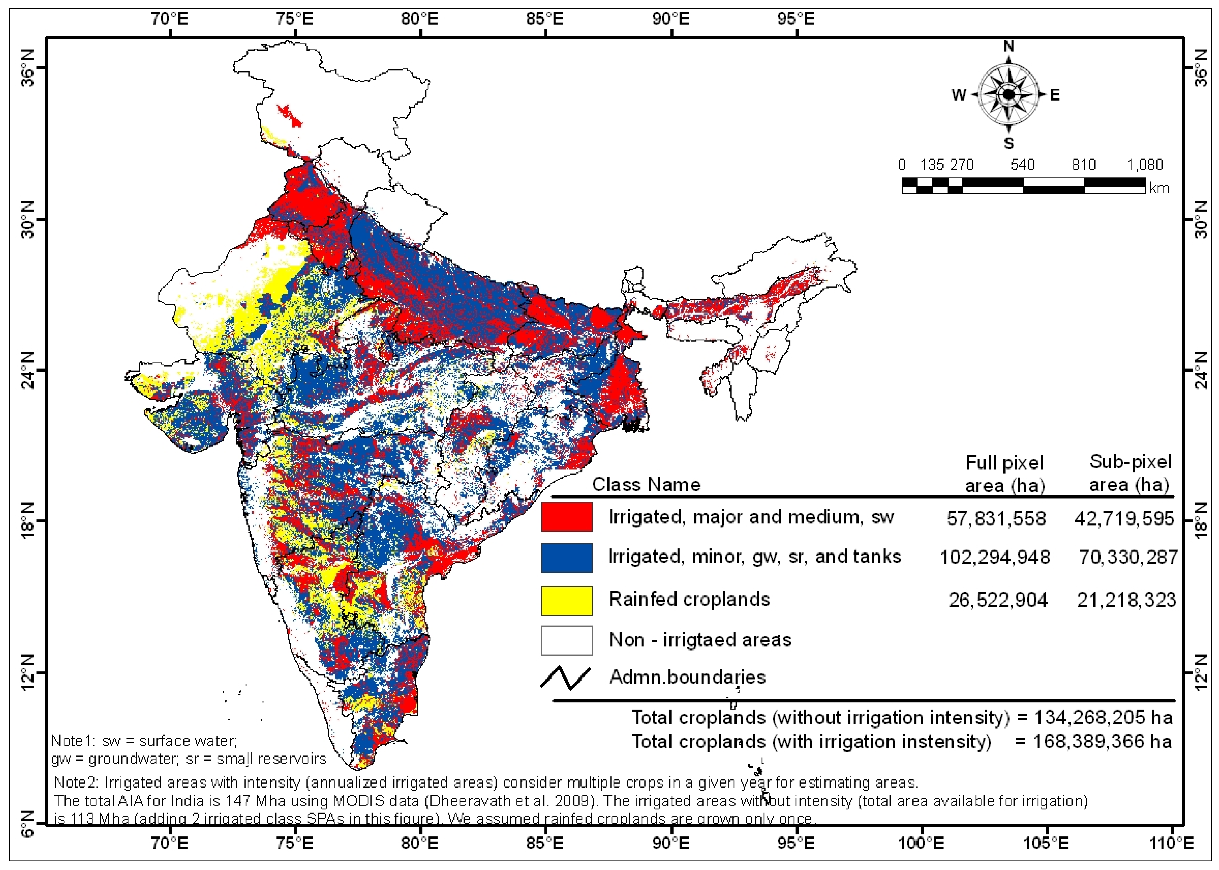
Figure 8. Cropland areas at higher spatial resolution of 500 m, which is adopted from Dheeravath et al. [63]. Cropland areas of India are determined using MODIS 500 m resolution time-series data of years 2001–2003. Generally, most studies agree that about 50% (or 164 Mha) of India’s geographic area (328.7 Mha) are croplands around year 2000.

Fifth, there are several studies in mapping croplands using improved resolutions of 500 m MODIS [16,63,73] , or conventional agricultural statistics [74] but none of these are at the global level. These products continue to propagate uncertainties in cropland areas. These studies are mostly limited to the national or subnational level. Dheeravath et al. [63] produced a cropland (irrigated and rainfed) map of India (Figure 8) for 2001–2003 using MODIS 500 m time-series data along with a suite of secondary data and field-plot data. Thenkabail et al. [1,2] estimated total cropland areas of India as 150 Mha at 10-km, comparable to this 500 m finer resolution product. However, most studies [1,52] disagree on the (a) proportions of irrigated to rainfed croplands and (b) precise location of croplands. The total area available for irrigation or TAAI (cropping intensity not considered) was 113 Mha whereas the annualized irrigated areas or AIA (the intensity considered) was 147 Mha. There is a high correlation between areas derived from the MODIS 500 m product [63] and AVHRR 10-km product [1,2] (Figure 9).

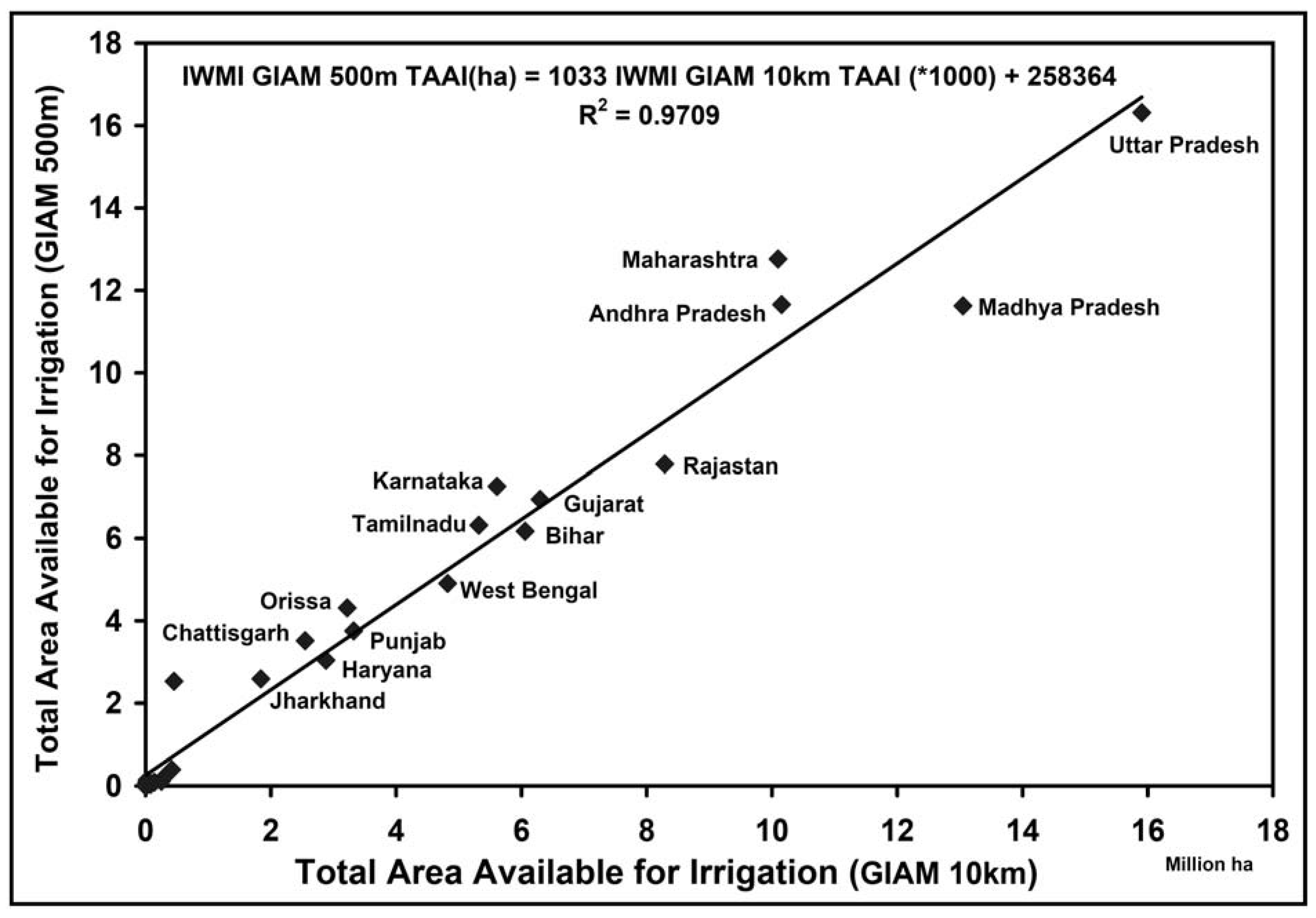
Figure 9. Irrigated croplands at two resolutions in India [63]. There is a remarkable correlation (R² value of 0.97) in irrigated areas mapped at nominal 10-km [1,2] versus irrigated areas mapped at MODIS 500 m [63]. However, areas estimated by MODIS 500 m were significantly higher for a few Indian states. This resulted in higher area estimates from MODIS 500 m data compared to the 10km product. Using MODIS 500 m, the total area available for irrigation or TAAI (the intensity not considered) was 113 Mha whereas the annualized irrigated areas or AIA (the intensity considered) was 147 Mha. These figures are significantly higher than Thenkabail et al. [1,2] estimated figures at 10-km of TAAI at 101 Mha and AIA at 132 Mha.

However, the MODIS derived areas were significantly higher than Thenkabail et al. [1,2] estimated areas at 10-km grid, TAAI of 101 Mha and AIA of 132 Mha. The cropland areas of India estimated using 10-km data were 203 Mha of TAAI and 243 Mha of AIA (Table 1), significantly higher figures than census based cropland statistics reported in the FAOSTAT as 168 Mha for year 2000 or 184 Mha reported by Portmann et al. [41] and Siebert and Döll [49]. The cropland statistics of 152 Mha reported by NRI (1997) for USA (Figure 10) are very close to Thenkabail et al. [1,2] reported 158 Mha but significantly higher than Portmann et al. [41] and Siebert and Döll [49] reported 131 Mha (Table 1). These results show that there is a need for more rigorous and consistent approach to overcome these limitations.

Figure 10. Cropland areas using non-remote sensing approaches with each dot representing 25,000 acres [74]. Cropland areas of USA are determined using various statistical data by NRI. Total cropland areas of USA is 152.56 Mha [74]. Thus about 15.86% of USA’s geographic area (963.1 Mha) are croplands around the year 2000. Thenkabail et al. [1,2] estimates 161.6 Mha. Irrigation intensity actually reduces this area to 157.8 Mha because there is overwhelmingly only one irrigated crop and during this period some of the land is left fallow. Map available at: http://www.nrcs.usda.gov/technical/nri/maps/meta/ m4964.html.

Sixth, Liu et al. [58] even used Landsat 30 m data to produce a cropland map of China (Figure 11). Their estimated cropland area of China for nominal year 2000 was 141 Mha—a figure lower than the FAOSTAT estimate of 160 Mha and Portmann et al. [41] and Siebert and Döll [49] reported 168 Mha (Table 1). It is difficult to say which estimate is more accurate. Liu et al. [58] study relied solely on one time Landsat data, which again can be a limitation. This implies that, we will not only need finer spatial resolution, but also higher temporal frequency (e.g., MODIS) to narrow the range of uncertainty and increase the reliability of estimates.

Figure 11. A cropland distribution map of China at 30 m resolution adopted from [58]. Cropland areas of China are determined using Landsat TM 30 m resolution data for 1990–2000. Total cropland areas of China is 141.1 Mha [58]. Thus about 14.35% of China’s geographic area (982.6 Mha) are croplands around the year 2000. This estimate by Liu et al. [58] is lower than 203.8 Mha estimated by Thenkabail et al. [1,2]. This does not include the intensity of irrigated areas which will add an additional 40 Mha [1,2].

5. Way Forward in Cropland Mapping

Given the above issues with existing maps of global croplands and specifically irrigated and rainfed areas, the way forward will be to produce global irrigated and rainfed areas at finer Landsat 30 m resolutions. Research has shown that at finer spatial resolution the accuracy of irrigated and rainfed area class delineations is better because more fragmented and smaller patches of irrigated and rainfed cropland can be delineated [75,76]. Further, crop types can be determined using finer spatial resolution. This is crucial for determining crop water use, crop productivity, water productivity, biomass yield, and carbon assimilation and sequestration potential in agriculture as well as a number of other applications at local, regional, continental, and global scales, making these products invaluable for research and development purposes. Since the sophisticated orthorectified Landsat Geocover images for the entire world [77] are available for free for the nominal years 1975s, 1990s, 2000s, and 2005s, global irrigated and rainfed cropland area maps at 30-m resolution are possible for these epochs. However, the Landsat images will have to be fused with Moderate Resolution Imaging Spectroradiometer (MODIS) 500-m time-series images in order to obtain time-series spectra that are so crucial for monitoring crop growth dynamics and cropping intensity (e.g., single crop, double crop, continuous year round crop).

Figure 12. Illustrating the challenges of global mapping at higher spatial resolution. Distribution of Landsat 30 m images for the world. About 9,500 images are required to cover the terrestrial world, with a total data volume of about 20 TB. With advanced compression techniques this can be reduced to about 4 TB. Yet, single shot Landsat images need to be fused with time-series imagery such as MODIS 250 m or 500 m for a realistic analysis of croplands or other land use. This further adds to data volume. Further, processing such high volume data brings its own challenges. This will require us to use super computer facilities. Image Credit: Mr. Manohar Velpuri, South Dakota State University, South Dakota, USA.

However, there are significant challenges in terms of data volume as well as data processing that need to be addressed. For instance, the uncompressed volume of the 9,770 Landsat Geocover reflectance images (Figure 12) of the entire world is about 20 terabytes, which must be compressed to a more manageable size. Some compression techniques include: (a) JPEG2000 lossless compression using ERMapper software [78]; (b) principal component analysis (PCA); (c) vegetation indices; and (d) focus on irrigated areas mapped by IWMI GIAM 10-km [2]. The JPEG2000 lossless compression, retaining all six nonthermal Landsat bands, reduces the volume for the global mosaic from about 20 TB to 4.8 TB, yet retaining the integrity of original reflectance values. Further, a massive reduction in global data volume is possible by several different approaches. First, taking only the irrigated and rainfed areas of the world as mapped in GIAM 10 km and in the global map of rainfed cropland areas (GMRCA 10 km)—both produced by IWMI (the statistics of which are also available at http://www.iwmigiam.org). The greatest confusion for irrigated areas comes from rainfed croplands. Putting the GIAM and GMRCA maps together, a total of about 1,500 Mha are covered, but often as blocks of fragments and not all contiguous areas. The GIAM and GMRCA areas are covered by roughly 1,000 Landsat images (down from the global coverage of 9,770 images), which reduced the data volume of the world to about 1.5 TB for 6-band reflectance images and a very manageable 360 gigabyte compressed JPEG2000 6-band image mosaic.

There is growing literature on global cropland (irrigated and rainfed) mapping across resolutions [1,2,43,76,79,80,81,82,83,84,85]. Based on these experiences, an ensemble of methods that is considered most efficient includes: (a) spectral matching techniques (SMTs) [1,2]; (b) decision tree algorithms [46]; (c) Tassel cap brightness-greenness-wetness [86,87,88]; (d) Space-time spiral curves, Change Vector Analysis (CVA) [54]; (e) Phenology [43,82]; and (f) fusing climate data with MODIS time-series spectral indices and using algorithms such as decision tree algorithms, and subpixel calculation of the areas [73].

The advanced and finer irrigated and rainfed croplands products at 30 m will: (1) define more precisely the actual area and spatial distribution of irrigated and rainfed cropland areas of the world; (2) develop methods and techniques for consistent and unbiased estimates of irrigated and rainfed cropland areas over space and time for the entire world; (3) elaborate on the extent of multiple cropping over a year, particularly in Asia, where two or three crops may be grown in one year, but where cropping intensities are not accurately known or recorded in secondary statistics; and (4) account for: (a) irrigation and rainfed cropping intensity; (b) irrigation source; (c) irrigated and rainfed crop types; and (d) precise location of irrigated and rainfed cropland areas. This will be a significant advance since irrigated and rainfed cropping intensity and their crop types have a huge influence on the quantum of water consumed by crops and associated indicators of agricultural productivity, crop diversification and food security. The irrigation and rainfed source is a must to determine patterns of land and water use and environmental impacts from factors such as major versus minor irrigation, and in determining the quantum of groundwater use and its overdraft issues that are critical to the food security and wellbeing of millions around the world, particularly in India and China. These two countries are home to largest number of poor and food insecure people worldwide; they are also the countries that encounter greatest gaps in data on cropping intensity and precise location of irrigated versus rainfed croplands. Precise and finer delineation of crop types, irrigation types and cropping intensities can greatly support global food security assessment and planning.

6. Global Cropland Water Requirements and Withdrawal: Blue, Green, and White Water

Croplands have resulted in changes in land use and cover through land clearing, specialization in production such as crop monoculture as well as deforestation and reforestation, deriving redistribution of evapotranspiration, decreasing it in areas of large-scale deforestation and increasing it in many irrigated areas with associated impacts on microclimate and regional climate impacts [89]. Continued increase in demand for water and recent water shortages have intensified the need for better utilization of our water resources; its has also forced us to think more innovatively about different components of water available in the hydrological cycle, including white, green, and blue water [90,91,92]. The blue, green and white water metaphor has enhanced policy discussion regarding water scarcity and food security.

Blue water: water in lakes, reservoirs, rivers, ice caps, and ground-water (saturated zone) are called “blue water”. However, the proportion of the water that evaporates back without being used by humans is called “white water”. Blue water is typically associated with crop production under irrigated conditions. The distinction between blue and white water has many implications for water management for food security. For instance, the lesser the blue water used for producing food and fiber the greater will be the water productivity and water use efficiency; however the implications for the environment may not always be straightforward.

Green water (productive green water or effective rainfall): water in the soil moisture that transpirates through crops and vegetation is termed “green water” since this water is available for crop productivity and vegetation. This water is in the unsaturated zone and readily available for consumptive use by crops. Green water is typically associated with crop production under rainfed conditions and constitutes bulk (70%) of the water used by croplands. The lesser the “green water” used for producing food and fiber crops the greater will be the water productivity. Strategies that improve green water management offer potential to enhance food production even in places with serious water scarcity issues [93].

White water (nonproductive green water or noneffective rainfall): Water that evaporates straight back to atmosphere from soil, water surfaces, and intercepted water from plant and other surfaces is termed as “white water”. This water is “not available” for human uses and recycles back into hydrological cycle, without being used.

Siebert and Döll [49] proposed a global crop water model (GCWM) to compute green water and blue water use of crops (Table 2, Figure 13). Basing their calculations on MIRCA2000 dataset [94] that provides monthly growing areas of 26 crops for 1998–2002 period, they estimated that the global total crop water use for the above mentioned period was 6,685 km³ yr−¹; of which blue water use was 1,180 km³ yr⁻¹, green water use of irrigated crops was 919 km³ yr⁻¹ and green water use of rainfed crops was 4,586 km³ yr⁻¹ (Table 2).

These data are comparable to the estimates of Falkenmark and Rockström [91]. Total crop water use was largest for rice (941 km³ yr⁻¹), wheat (858 km³ yr⁻¹) and maize (722 km³ yr⁻¹). The largest amounts of blue water use were for rice (307 km³ yr⁻¹) and wheat (208 km³ yr⁻¹) [49]. Postel [95] estimated the total volume of water consumed for food production, roughly at the end of the last millennium as 13,800 km³/yr of which 7,500 km³/yr goes for food crops and their associated biomass (higher than Siebert and Döll, [49] and Falkenmark and Rockström [91] estimates, but it includes “associated biomass”) and the rest 5,800 km³/yr for pasture and natural grazing lands. This is about 20% of the total evapotranspiration per year from Planet Earth [95].

Falkenmark and Rockström [91] suggest that much of the water for food security in next few decades will have to come from green water, with irrigation withdrawal plateauing or even exceeding annual fresh water recharge in some areas such as parts of Yellow River Basin in China and Indo-Gangetic Basin and also becoming increasingly unacceptable due to severe impacts on environments and ecologies [14].

Figure 13. Blue water-green water approach [91]. About 20% of all water used for crops comes from the blue water diversions (from water in lakes, reservoirs, rivers, and ground water in aquifers) irrigating 278–399 Mha (without intensity) and 467 Mha (with intensity) annually. There is an additional 10% of water from direct rainfall (green water) over irrigated croplands. The rest, about 70%, of water used by crops is the green water (water in soil moisture in unsaturated zone) used by about 1.13 billion hectares of rainfed croplands. Management strategies for blue and green water are not the same and the impacts on food security depend synergistically on how blue and green water is managed and for what crops and where.

Note: about 80% of all blue water diversions for human water use goes to produce food by irrigated croplands. The 278.4 Mha is the global irrigated area determined by Siebert et al. [52] and 399 Mha is the global irrigated area determined by Thenkabail et al. [1,2]. The 20% blue water use by irrigated lands is based on Siebert et al. [52].

Table 2. Global blue water and green water use by agricultural crops roughly at the end of the last millennium.

**Table 2.** Global blue water and green water use by agricultural crops roughly at the end of the last millennium.
Blue water use by irrigated crops km³/yr	Green water use by irrigated crops km³/yr	Green water use by rainfed crops km³/yr	Total water use by irrigated crops rainfed crops km³/yr	Reference
1,180	919	4,586	6,685	Siebert and Döll [49]
1,800	–	5,000	6,800	Falkenmark and Rockström [91]
–	–	–	7,500	Postel [95]

Irrigated areas consume nearly 80% of all human blue water use by humans. A country by country irrigated crop water requirement is computed by Siebert and Döll [49] (Table 3). They first compute the direct rainfall (green water) over irrigated areas and then compute the additional irrigation requirements (blue water) to sustain the crop during its growing period. Water required is the evapotranspiration of crops assuming optimal crop growth and no water limitation [49]. Green water is just the part of evapotranspiration that is provided by direct rainfall and blue water required is the additional evapotranspiration that occurs on irrigated fields as compared to rainfed conditions (assuming optimal growth and no water limitation on irrigated fields) (Siebert, personal communication). Adding these two water components over irrigated areas, gives the total irrigated crop water requirement, presented for 197 countries by Siebert and Döll [49] (Table 3).

Figure 14. Water required by crops [49,97]. Water required by irrigated croplands shown here includes green water (direct precipitation over the irrigated areas) plus additional blue water required (water from lakes, rivers, reservoirs, and ground water from aquifers) for sustaining crops. The highest water use (500 mm or more) is in the Ganges basin (India), Indus basin (Pakistan), areas near Beijing (China), and California valley (USA). High water use occurs in areas with high irrigation density, cropping intensity, and evaporative demand as noted in the figure. The irrigated areas used to compute water required are from MIRCA2000 data set (www.geo.uni-frankfurt.de/ipg/ag/dl/forschung/MIRCA/index. html) which is derived from Siebert et al. [52].

In contrast, Wisser et al. [96] determined a country-wise “water withdrawal”. Typically, much more water is withdrawn for irrigation than crop water requirements, leading to poor irrigation efficiency. As a result water productivity (WP) can vary widely based on how water use is determined. Water input through canals is often far higher than water used by crops due to evaporative losses during supply and through direct evaporation from standing water in the field and percolation or infiltration. So, if we calculate WP based on water supplied it is likely to be 2–3 times lesser than the WP calculated based on water use by crops. To fully account for various components of water withdrawals, a basin perspective is required to analyze water productivity.

A country-wise comparison of water withdrawals for irrigation per year [96] is made with the corresponding country-wise water requirements estimated by Siebert and Döll [49] (Figure 14 and Table 3). Siebert and Döll [49] used irrigated areas reported in Siebert et al. [52] to estimate water required for optimal cropping conditions. Wisser et al. [96] used irrigated areas reported in Siebert et al. [52] (Figure 4, Table 1) and Thenkabail et al. [2]. The results in Figure 15 and Figure 16 indicate that, on an average, 1.6 to 2.5 times more water is withdrawn than required for irrigation, thus achieving irrigation efficiency of just 40% to 62%.

Figure 15. Water withdrawal [96] versus water required [49,97] by irrigated crops for 197 countries in the World. Water withdrawals are, of course, always much higher than water required. Here the trend shows withdrawal, on average, to be about 1.6 times than the water required for irrigation. The irrigated areas used to compute water withdrawal and water required are both from Siebert et al. [52].

Figure 16. Water withdrawal [96] versus water required [49,97] by irrigated crops for the 197 countries in the World. Water withdrawals always much higher than water required. Here the trend shows withdrawal, on average, to be about 2.5 times the water required for irrigation. The irrigated areas used to compute water withdrawal are from Thenkabail et al. [1,2] and water required are from Siebert et al. [52].

7. Virtual Water Use

There is an increasing trend to regard water as a commodity that can be traded across basins, regions, nations, and continents. Virtual water use describes the water used to produce food crops that are traded [98,99]. Several authors [100,101,102,103,104] have described how water short countries can enhance their food security by importing water intensive food crops. Thus water surplus countries can produce food and export to water scarce countries, to the comparative advantage of both. Virtual water use improves the physical and economic access to food by increasing food availability and reducing food prices for domestic consumers. It also enables the global exchange of surplus food. In other words, it improves entitlements through exchange and, in so doing, widens the range of food available for consumption, improving diets and satisfying food preferences. Van Hofwegen [105] observed that virtual water trade is already a silent alternative for most water-scarce countries as it could be used as an instrument to achieve water security but also because of its increasing importance for food security in many countries with a continuous population growth. The virtual water trade addresses resource endowments but it does not address production technologies or opportunity costs of trade [98,99]. Optimal trading positions are therefore not always consistent with expectations based solely on resource endowment. The trading positions are determined by geopolitical and economic factors and some nations may not have the economic capacity to pay for virtual water food imports.

Table 3. Global water withdrawals versus water use by croplands—a country by country assessment. Also, blue water and green water use of irrigated croplands.

**Table 3.** Global water withdrawals versus water use by croplands—a country by country assessment. Also, blue water and green water use of irrigated croplands.

For instance, virtual water trade increases with increase in cropped area; access to croplands must increase to help utilize available blue water for irrigation. This means that many of the humid, water-rich countries will not be in a position to produce surplus food and feed the water scarce nations. Others empirically argue that virtual water trade increase only with increase in gross cropped area and what is often achieved through virtual water trade is “global land use efficiency”. Accordingly, for a water-poor, but land-rich country, virtual water import offers little scope as a sound water management strategy [106]. Global croplands remain critical even for the virtual water use strategies.

Globally, there is sufficient fresh water to meet human needs, including for food production, for foreseeable future. However, its distribution is uneven and timing of precipitation is concentrated in few months in many parts of the world. The virtual water concept is expected to help in better water management by taking the globe as a unit. Estimates suggest that some 695 Gm³ yr⁻¹ [one Gm³ or giga-cubic meter is one billion cubic meters or one trillion (1 × 10¹²) liters] or about 11% of the water used by crops (6,685 Gm³ yr⁻¹; Table 1) was virtually traded at the end of the last millennium [107].

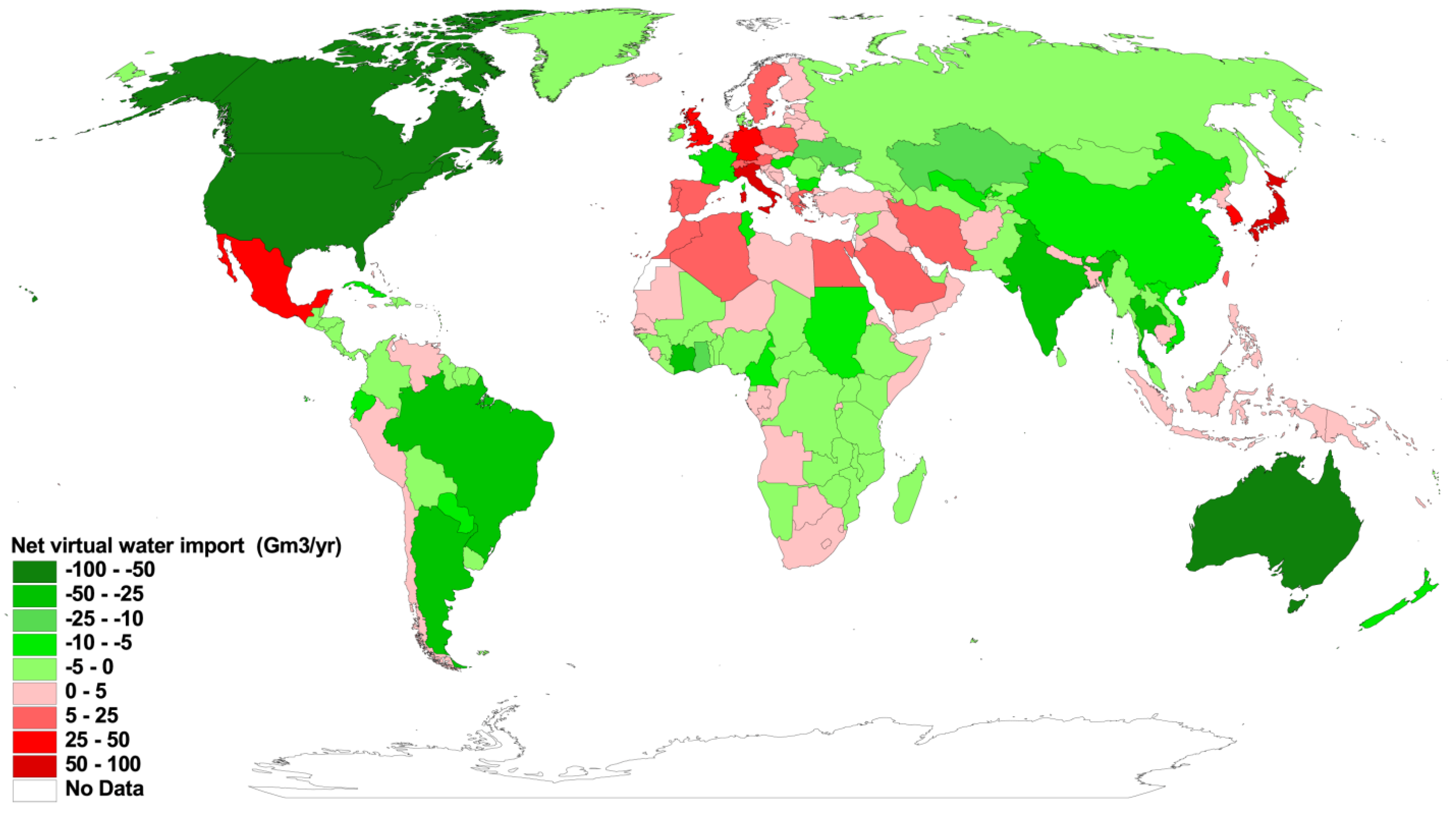
Figure 17. Virtual water balance per country over the period 1997–2001 [107]. The balances are drawn based on an analysis of international virtual-water flows associated with trade in both agricultural and industrial products. The red-colored countries have net virtual-water import; the green-colored countries have net virtual-water export.

The countries with the largest net virtual water export are Australia, United States, Canada, Thailand, Argentina and India [108] (Table 4a). The largest net importers are Japan, Italy, Germany, South Korea, China and Indonesia [108] (Table 4b). For example, Germany alone, with current policy on biofuel importation, will require an additional 2.5–3.4 Mha of cropland by 2030, possibly through land use conversions in Brazil or Indonesia [109]. This in turn will result in an additional 23–37 Tg of CO₂.

Table 4a. Top-15 of gross virtual water exporters and top-15 of gross virtual water importers for the period: 1997–2001 [Source: Hoekstra, A.Y.; Chapagain, A.K. Globalization of water: Sharing the planet's freshwater resources: Blackwell Publishing, Oxford, UK, 2008].

**Table 4a.** Top-15 of gross virtual water exporters and top-15 of gross virtual water importers for the period: 1997–2001 [Source: Hoekstra, A.Y.; Chapagain, A.K. Globalization of water: Sharing the planet's freshwater resources: Blackwell Publishing, Oxford, UK, 2008].
Top gross exporters		Rank	Top gross importers
Countries	Gross export		Countries	Gross import
Countries	(Gm³/yr)		Countries	(Gm³/yr)
USA	229	1	USA	176
Canada	95	2	Germany	106
France	79	3	Japan	98
Australia	73	4	Italy	89
China	73	5	France	72
Germany	71	6	Netherlands	69
Brazil	68	7	United Kingdom	64
Netherlands	58	8	China	63
Argentina	51	9	Mexico	50
Russia	48	10	Belgium-Luxembourg	47
Thailand	43	11	Russia	46
India	43	12	Spain	45
Belgium-Luxembourg	42	13	Korea Rep.	39
Italy	38	14	Canada	35
Cote d’Ivoire	35	15	Indonesia	30

Note: One Gm³ or giga-cubic metre is one billion cubic metres. This contains one trillion (1,000,000,000,000 or 1 × 10¹²) litres.

Table 4b. Top-10 of net virtual water exporters and top-10 of net virtual water importers for the period 1997–2001. [Source: Hoekstra, A.Y., Chapagain, A.K., Globalization of water: Sharing the planet's freshwater resources: Blackwell Publishing, Oxford, UK, 2008].

**Table 4b.** Top-10 of net virtual water exporters and top-10 of net virtual water importers for the period 1997–2001. [Source: Hoekstra, A.Y., Chapagain, A.K., Globalization of water: Sharing the planet's freshwater resources: Blackwell Publishing, Oxford, UK, 2008].
Countries with net export	Virtual water flows (Gm³/yr)			Rank	Countries with net import	Virtual water flows (Gm³/yr)
Countries with net export	Export	Import	Net export	Rank	Countries with net import	Import	Export	Net import
Australia	73	9	64	1	Japan	98	7	92
Canada	95	35	60	2	Italy	89	38	51
USA	229	176	53	3	U/Kingdom	64	18	47
Argentina	51	6	45	4	Germany	106	70	35
Brazil	68	23	45	5	South Korea	39	7	32
Ivory Coast	35	2	33	6	Mexico	50	21	29
Thailand	43	15	28	7	Hong Kong	28	1	27
India	43	17	25	8	Iran	19	5	15
Ghana	20	2	18	9	Spain	45	31	14
Ukraine	21	4	17	10	Saudi Arabia	14	1	13

Note: One Gm³ or giga-cubic metre is one billion cubic metres. This contains one trillion (1,000,000,000,000 or 10¹²) litres.

8. Croplands, Crop Water Availability, Climate Change, and Food Security

Global climate change is a serious threat to world food security. Declining per capita global food production and warming oceans threaten food security [16]. Climate change also challenges our scientific understanding of the existing hydrological and biophysical relationships of water and food production and requires costly adaptation of core water programs and policies to unprecedented changes, impairing human capacity to respond to climate change. Adequate cropland supported by adequate water availability is essential for food security. What is “adequate” depends on how much we can produce per unit of land (crop productivity expressed in kg/m²; CP) and how much we can produce by a unit of water (water productivity expressed in kg/m³; WP). The Green Revolution (from 1960–2000) was made possible by the four main factors: (a) continued increase in crop productivity; (b) expansion in cropland areas; (c) intensification of cropping (more than one crop in a year); and (d) irrigation expansion at a rapid rate [110], all supported by pro-food government policy and assistance from international donors [111]. However, all these factors have now stagnated or are increasing at a rate almost insignificant compared to the Green Revolution period. The donor assistance and lending to agricultural research have faded and hit all times low. Population growth and economic growth continue to derive income transition for a far wider segment of society particularly in China and India, raising demand for calorie intake per person, influencing dietary changes and transforming the way the global cropland and water resources must be used to produce food. This compounds the perplexing climate change challenges.

A serious threat to future food security comes from a changing climate and related uncertainties in water availability. This is illustrated for the case example of Krishna river basin in India (Figure 18) by considering a water water-surplus year (2000-01) and comparing it to a water-deficit year (2002-03). The change in the net area irrigated was modest with an irrigated area of 8,669,881 hectares during the water-surplus year when compared with 7,718,900 hectares during the water-deficit year [112]. However, this is quite misleading as it does not show most of the major changes that occur in the cropping intensity, changing from a higher to lower intensity (e.g., from double crop to single crop). The changes in cropping intensity of the agricultural cropland areas that took place in the water-deficit year (2002-03) when compared with the water-surplus year (2000-01) in the Krishna basin were [112] highly significant (see Figure 18) and have strong impact on food security. Thus significant adjustments in irrigated area, crop mix, crop productivity, and land use are likely under wet-dry conditions that occur in most river basins, including the Colorado River basin in US [113], Mekong Basin countries [114], Murray Darling Basin [115,116] and the Yellow River Plain in China [117], with implications for economic wellbeing of agricultural communities. Such changes may be expected in many parts of the world in a changing climate.

Figure 18. Food security in a changing water and climate scenario [112]. Irrigated cropland change map from 2000-01 (water-surplus year) when compared with 2002-03 (water-deficit year). Changes that occurred in a water-deficit year relative to a water-surplus year are shown in the map, including: (a) 1,078,564 hectares changed to single crop from double crop; (b) 1,461,177 hectares changed from continuous crop to single crop; (c) 704,172 hectares changed from irrigated single crop to fallow; and (d) 1,314,522 hectares from minor irrigation (e.g., tanks, small reservoirs) to rainfed.

9. A New Paradigm for Future Food Security

The Malthusian model of “Population, when unchecked, increases in a geometrical ratio while subsistence increases only in an arithmetical ratio” [118] is certainly not true for the Green Revolution period (1960–2000) when, actually, foodgrain production nearly tripled to just above two billion tons whereas population doubled from about 3 billion to about 6 billion; even though croplands decreased from about 0.43 ha/capita to 0.26 ha/capita [7]. This was mainly as the result of: (a) expansion in irrigated areas which increased from 130 Mha in 1960s to 278.4 Mha in year 2000 [52] or 399 Mha when you do not consider cropping intensity [1,2] or 467 Mha when you consider cropping intensity [1,2]; (b) increase in yield and per capita food production (e.g., cereal production from 280 kg/person to 380 kg/person and meat from 22 kg/person to 34 kg/person [119]; (c) new cultivar types (e.g., hybrid varieties of wheat and rice, biotechnology); and (d) modern agronomic and crop management practices (e.g., fertilizers, herbicide, pesticide applications).

However, the Malthusian vision comes back into sharp focus in the new millennium with continued population growth [9] and stagnated crop yield growth [120], diversion of croplands to biofuels [10], limited water resources for irrigation expansion [121], limits on agricultural intensifications, loss of croplands to urbanization [14], increasing meat consumption (and associated demands on land and water) [122], environmental infeasibility for cropland expansion [123], and changing climate. Indeed, some of the factors that lead to the Green Revolution have stressed the environment to limits leading to salinization and decreasing water quality. For example, from 1960 to 2000, the phosphorous use doubled from 10 million tons to 20 MT, pesticide use tripled from near zero to 3 MT, and nitrogen use as fertilizer increased to a staggering 80 MT from just 10 MT [14,124]. Further, diversion of croplands to biofuels is already taking water away from food production; the economics, carbon sequestration, environmental, and food security impacts of biofeul production are net negative [125], leaving us with a carbon debt [126,127].

Future security is threatened by the complex factors. The new food security paradigm must extend beyond current definition that includes food production/availability, access, affordability, and utilization and must encompass various drivers of global change, including climate change, as well as the outcomes of global change processes including impacts on global croplands and water resources, and global policy and institutional solutions afforded by the challenges ahead such as global carbon trading schemes and reducing emissions from deforestation and degradation (REDD) – an emerging strategy with big potential for mitigating the climate change but serious consequences for taking water away from food production to commercial forest plantations. It must consider croplands and associated agricultural arrangements in the context of a quest for a low carbon economy as well as the potential inclusion of agriculture into the carbon pollution reduction schemes worldwide [39]. Strengthening global and local governance is the key and food security must be closely connected with economic growth and social progress as well as political stability and peace. In addition, future food security agenda must also focus on:

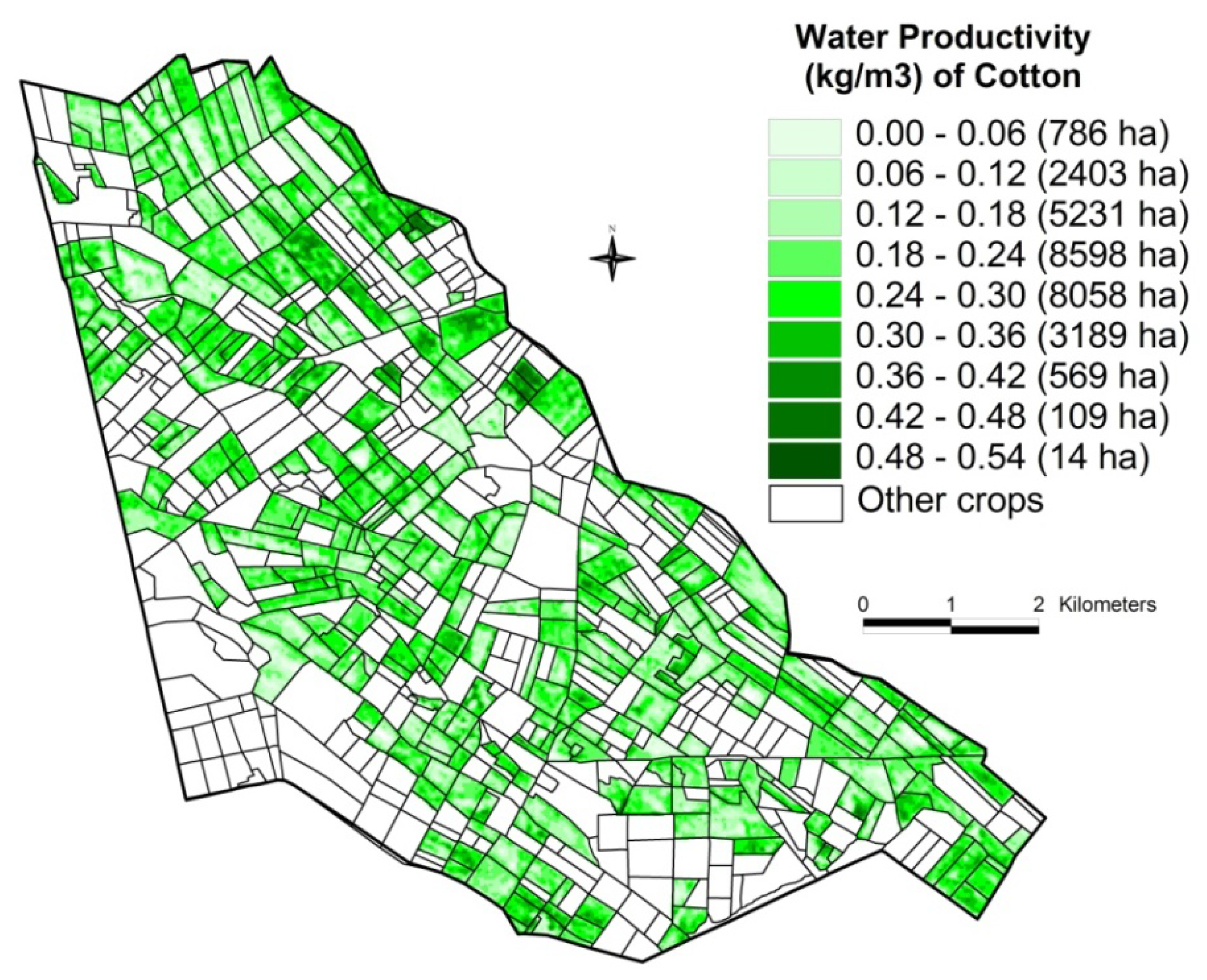
Improving water productivity (operationalize the concept of more crop per drop). Recent research by Platanov et al. [128] demonstrated that as high as 87% of all croplands in the intensively irrigated areas of Central Asia have low WP (e.g., Figure 19). Their research implied that there is an overwhelming proportion of cropland areas where better land and water management practices can help to improve WP, thus leading to food security without having to increase allocations of land and water resources [129].

Better agricultural technologies and cropping systems. The change in cropping pattern (e.g., more wheat than rice) can deliver significant gains in food security. For example, rice crop requires about 2,000 liters to produce 1kg of rice where as wheat requires half that amount. Currently, India produces about 93 million tons of rice per year requiring 178 km³ of water. Investments to convert 50% of rice area to wheat, will save about 45 km³ (or 45 trillion liters of water) every year.

Conserving water, preserving land resources. Enhancing the productivity of existing croplands and available blue and green water resources is the main pathway to future food security. This can be achieved through a suite of measures and approaches such as: (a) protecting croplands against salinization; (b) precision farming and resource conservation practices; (c) low-cost water saving irrigation innovations (e.g., drip, sprinklers); (d) reducing food waste from farm to fork that ranges anywhere between 20%–35% of all food produced [130], nutrient recovery and reuse; (e) desalination to augment water shortages (for urban water use is economically viable, but too costly for irrigation); (f) wastewater recycling (water reuse); and (g) and adopting organic farming that is more sustainable and also maintains the quality of land and water (thus, for example, increasing fish population).

Harnessing the potential of biotechnology. Genetically modified and non-GM crops that give better yields, are resistance to drought and are cold tolerant, can grow with less water, less number of growing days, and have better social acceptance can enhance food security. It has huge potential but the risks to environment and human health should be carefully assessed to safeguard the food security [131].

Policy planning and support for virtual water use/trade. Policy processes and WTO negotiations must create a level playing field for all stakeholders, particularly the poor countries heavily dependent on agriculture and unable to afford recurring food imports. For example, cotton will require 5,404 m³ of water per ton if produced in China whereas it requires 21,563 m³ per ton if produced in India (http://www.waterfootprint.com). Does that mean that we should grow some crops in some countries and have a global trade agreement? This is debatable as the issues of food security conflict with food sovereignty [132].

Figure 19. Water productivity map (WPM) illustrated for an irrigated area in Uzbekistan [128]. The the water productivity maps (WPMs) are derived by dividing the crop productivity maps (CPMs) with water use maps (WUMs). Nearly 87% of the areas is in the low water productivity (WP; <0.30 kg/m³). This shows the opportunity that exists to grow more food from existing croplands and existing water allocated for crops by just improving WP.

10. Conclusions and Policy Implications

This paper provided a comprehensive overview of the estimates of global cropland areas and their water use assessment for 197 countries; summarizing and comparing findings by world’s leading researchers on the subject. It argued that, global croplands remain key to ensuring future water and food security. At the end of the last millennium, world had between 1.47–1.53 billion hectares of croplands as per major remote sensing [1,2] and non-remote sensing studies [40,41,42,49,52]. Major cropland studies converge on these figures. A comparison of cropland areas of 197 countries between different studies had a high R²-value between 0.89–0.94. Further, a comparison of irrigated cropland areas of 197 countries by different studies showed even a higher R²-value between 0.94–0.97. These results indicate a presence of a strong trend between two products. However, there are significant differences in total cropland areas and/or their precise geographic locations for many individual countries between products that are not apparent in R²-values. For example, irrigated croplands are variously estimated as 278 Mha [52], 312 Mha [41], 399 Mha (without cropping intensity) [1,2], and 467 Mha (with the intensity) [1,2]. The differences in irrigated area estimates between different studies [1,2,41,52] were especially significant in major irrigated area countries like China and India. The causes of these differences were as a result of definitions used in mapping, data types used, methodologies used, resolution of the imagery, uncertainties in sub-pixel area computations, inadequate accounting of statistics on minor irrigation (groundwater, small reservoirs and tanks), and data sharing issues.

Global cropland’s water use vary between 6,685–7500 km³ yr⁻¹ [4,95,96]; with 70% as the green water used by about 1.13 billion hectares of rainfed croplands, 20% as the blue water used by about 278–399 Mha of irrigated croplands, and the 10% as the green water use by irrigated croplands from the rain that falls directly on these lands.

The croplands estimated by various approaches are still too coarse for appropriate planning of water use by crops. Thereby, the need for higher spatial resolution remote sensing products that offer numerous advantages including: (a) precise location of croplands; (b) delineation of crop types; (c) determining cropping intensity; (d) information on watering method (irrigation or rainfed); and (e) potential applications for food security planning and targeting investment to the food security hotspots. These facts clearly imply a need for high spatial resolution cropland mapping (and determination of associated water use) using advanced remote sensing. An ideal solution will be to produce a cropland map by fusing Landsat ETM+ 30 m data with MODIS time-series 250/500 m data. Knowledge of all these factors can have a huge impact on the quantum of water used and is also essential for improved climate change models. Such information becomes even more critical for water trade (virtual water) assessments and negotiating agricultural policy positions in a global change scenario and emerging global carbon trading regime.

A new paradigm for food security has been articulated. Global climate change, population growth, nutritional transition, and global environmental change are placing unprecedented pressure on global croplands and water use. A paradigm central for ensuring global food security in the 21^st century, when land and water become more limiting factors as populations and economies grow, have been articulated. First, a country-by-country comparison showed about 1.6 to 2.5 times the water required for irrigation is actually withdrawn from fresh water sources; making irrigation efficiency only 40%–62%. This is one area where huge potential to improve efficiency exists. Second, irrigated areas generally have low water productivity (WP; crop productivity per unit of water). Indeed, in heavily irrigated parts of Central Asia, about 80% of croplands are in low WP range. Generally, WP is low or very low in over 50% of World’s irrigated croplands. This is an area where large quanta of water can be saved by improving WP of low productivity areas. Third, a big water saving strategy could be to change crop types (e.g., grow more wheat than rice). For example, if we convert 50% of rice area of India to wheat, we could save about 45 km³ (45 trillion liters) of water every year. Fourth, is to improve crop productivity of rainfed croplands, through improved green water management which have received scant attention to-date. Fifth, reuse of wastewater and marginal quality water in agriculture and purifying water through reverse osmosis can also save large quanta of fresh water. Sixth, desalination is already becoming economically viable solution for urban and industrial water use. However, it is not yet economical for agriculture. Seventh, trading water as a commodity (e.g., virtual trade) within and between countries also offers potential to boost food security but issues involving food security versus food sovereignty require balancing. As per current water scenario, uneven water distribution globally is the real issue than real physical water scarcity. Eight, a number of other management measures (e.g., precision farming, waste reduction, organic forming that will preserve our soils and enrich alternative food chain like fish), and new biotechnology (e.g., crops with less growing period, improved seeds) must all be considered by the new food security paradigm. Ninth, above all, it must respond to the global climate change challenges. For example, the paper illustrates serious decrease in food production during a water-deficit year compared with a water-excess year for a key river basin. This is likely to exasperate under a climate change scenario and numerous competing demands on croplands and water use in the context of global environmental and economic change. It must also respond to the potential inclusion of agriculture into the global carbon trading regime and associated impacts on croplands, water use, food production and food entitlements under the emerging global social contract.

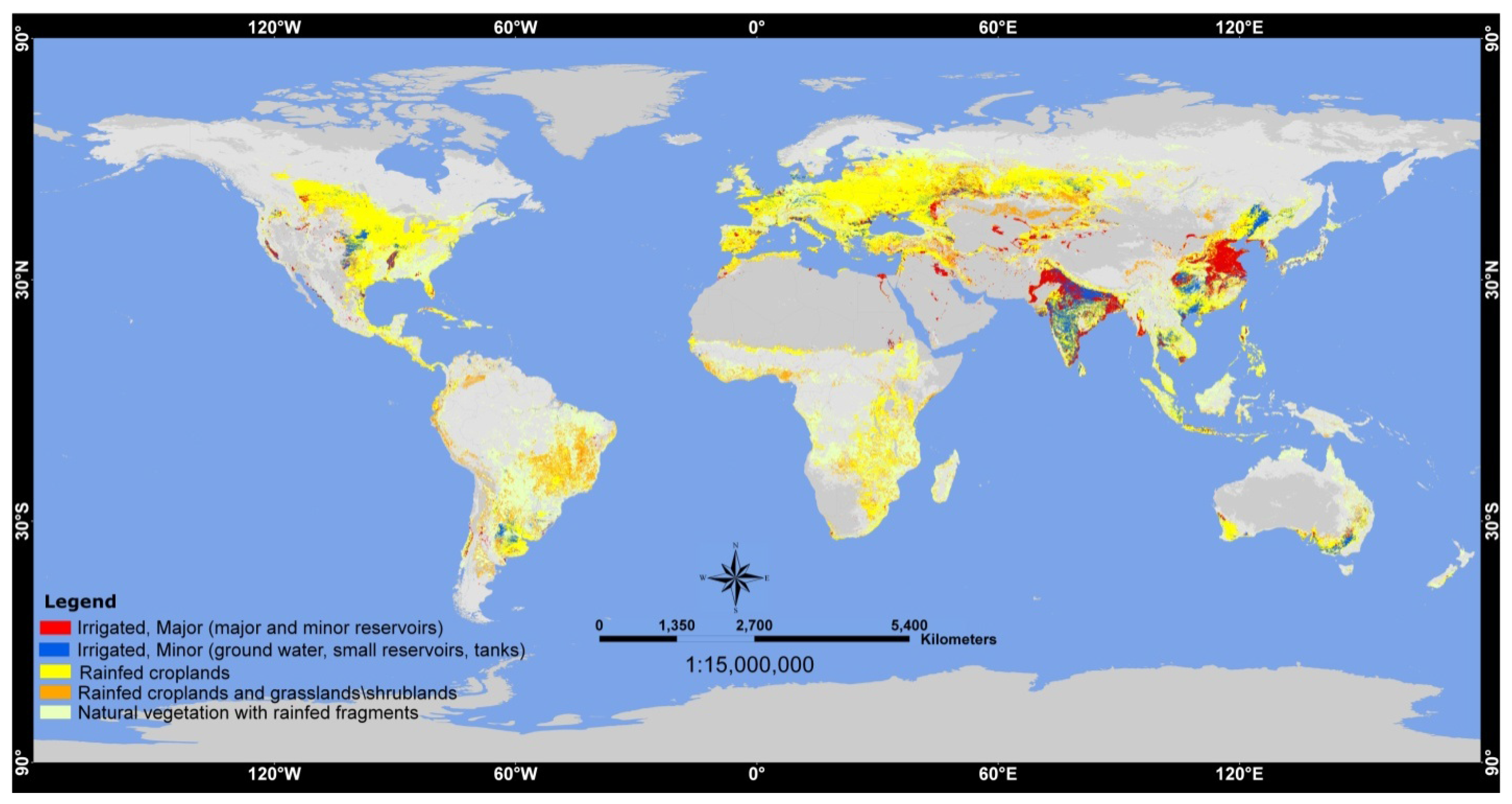
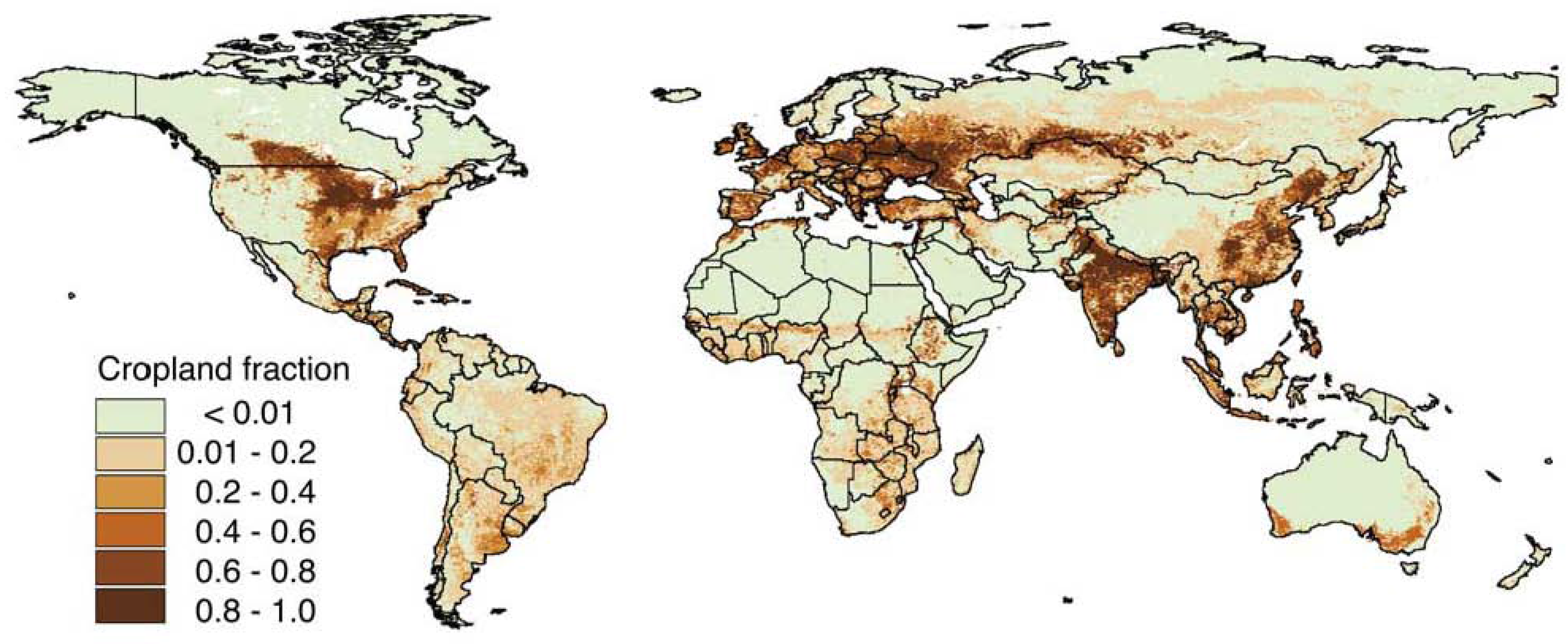
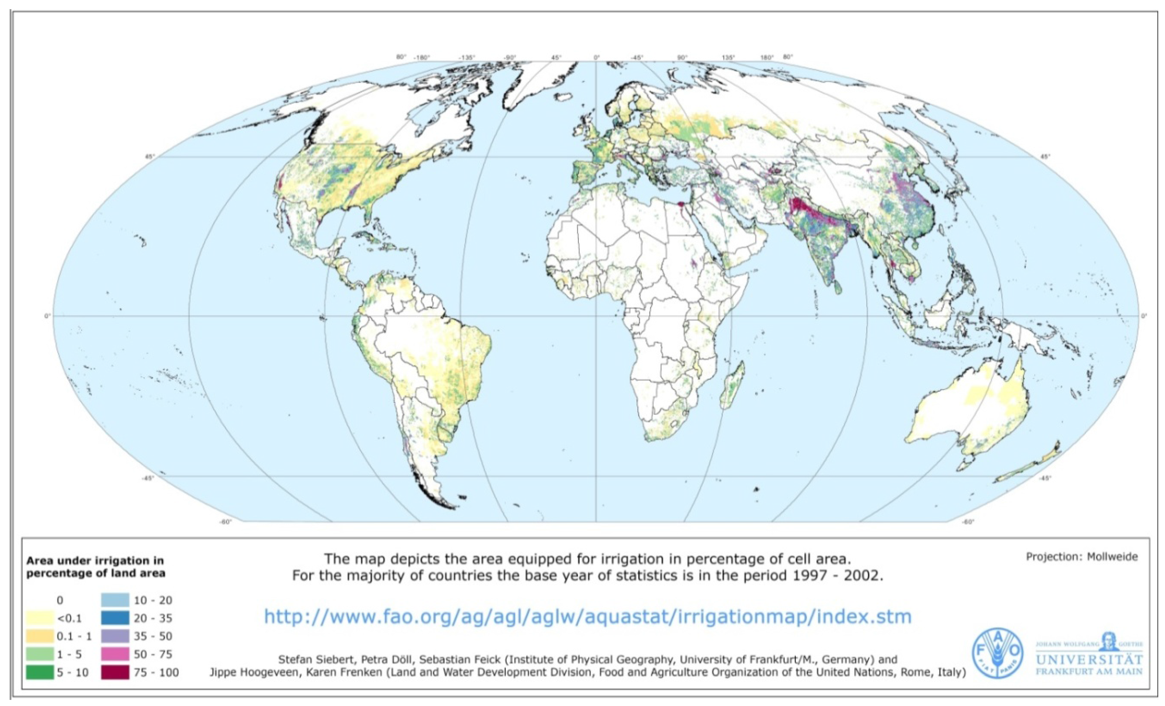
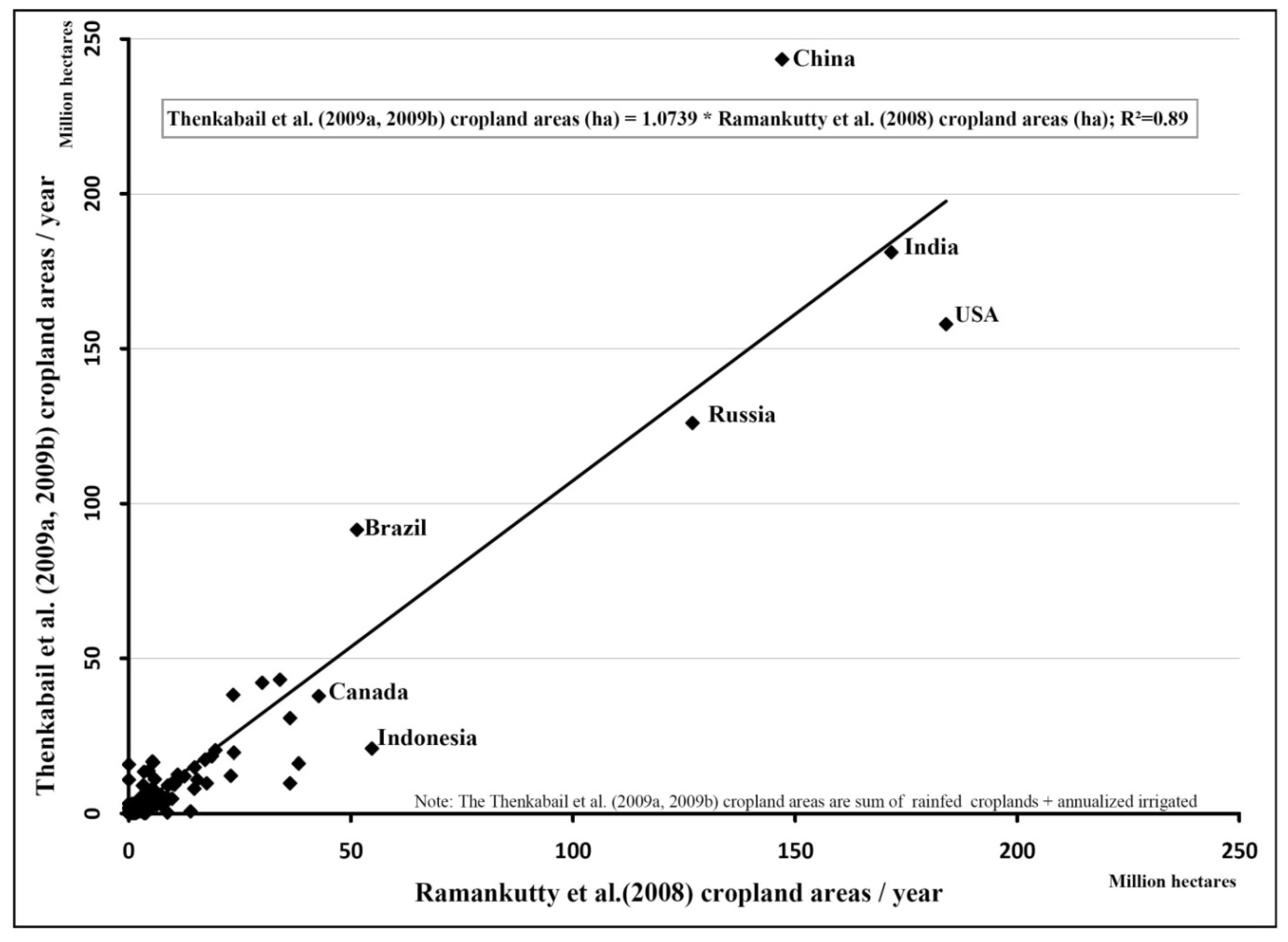
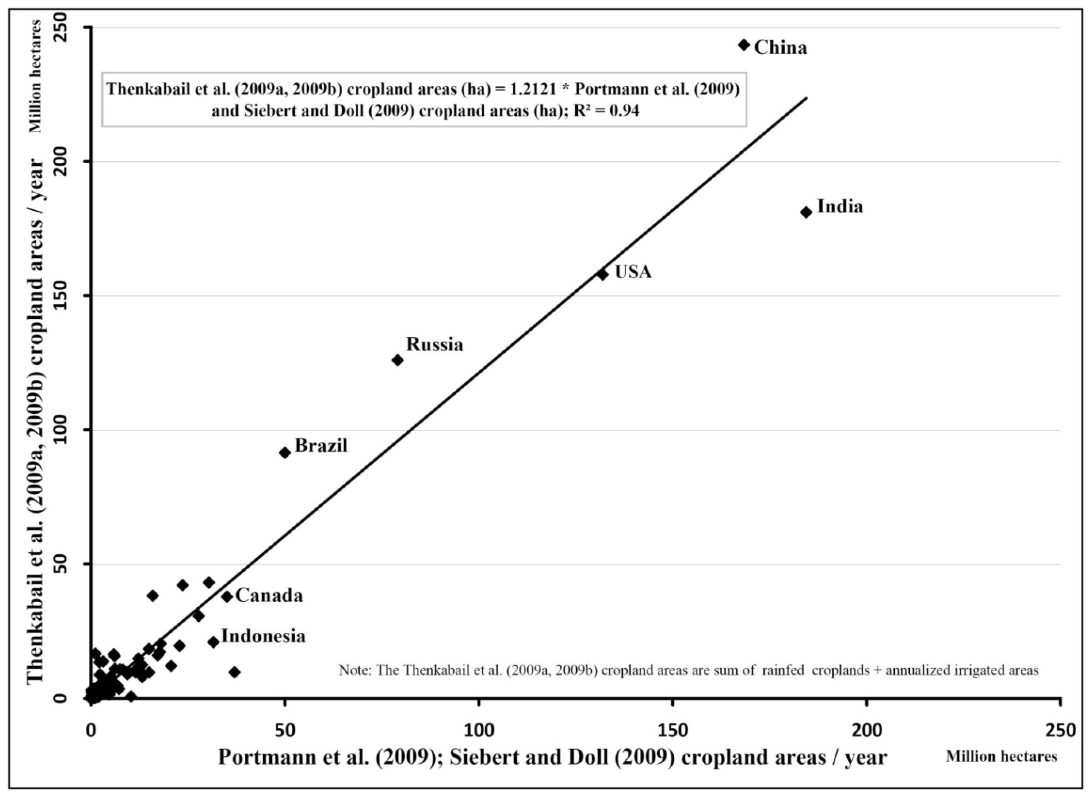
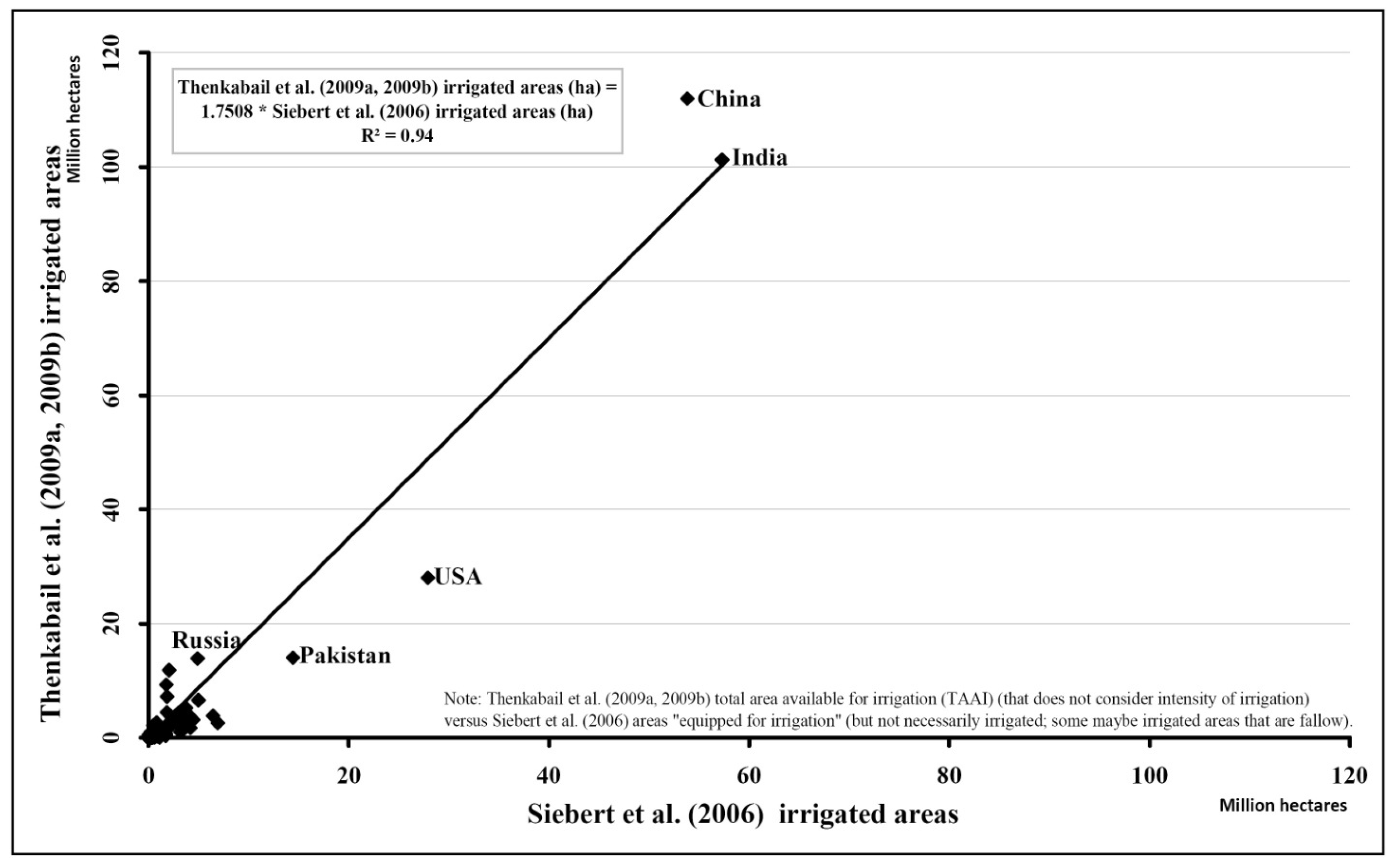
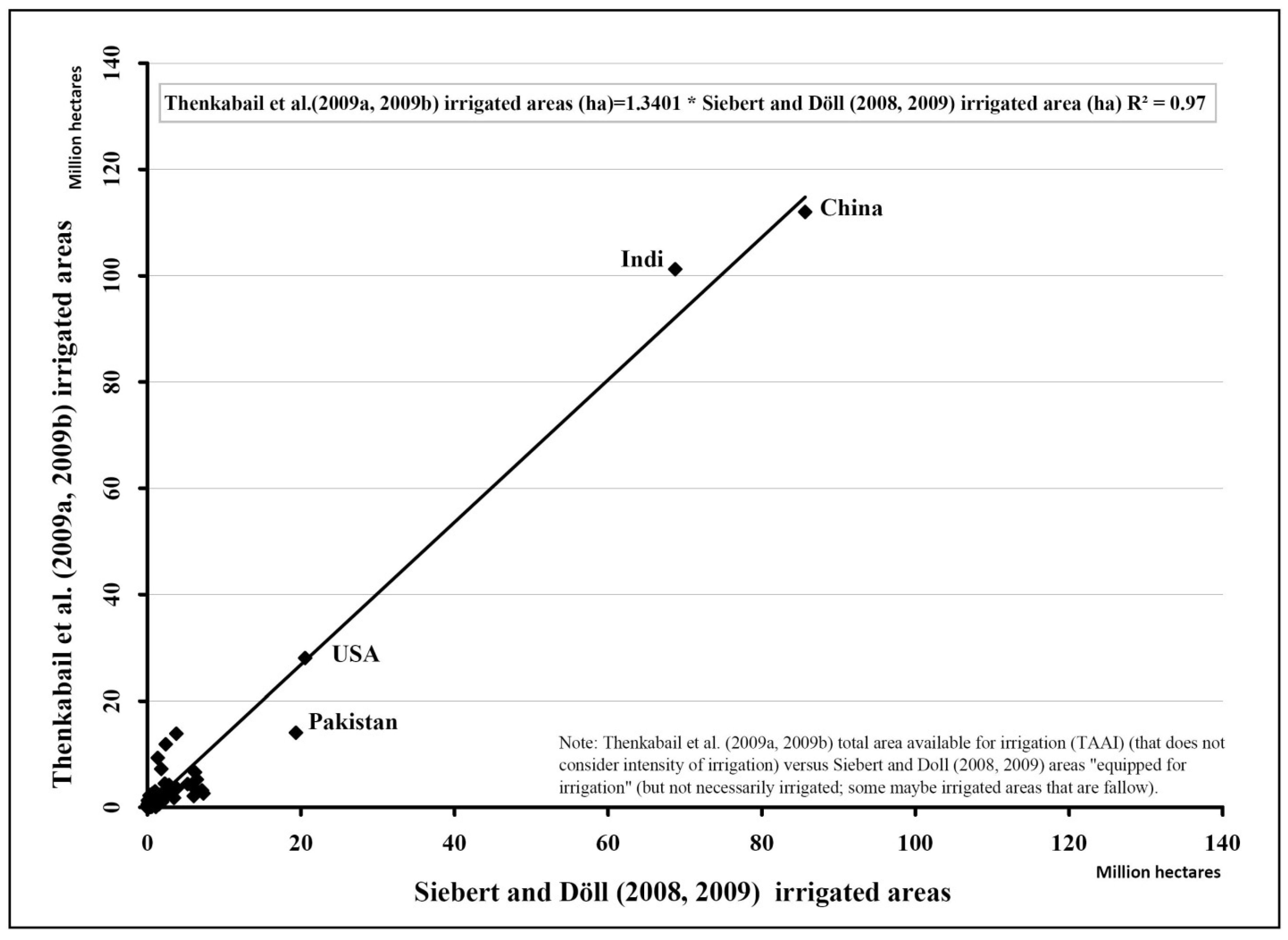
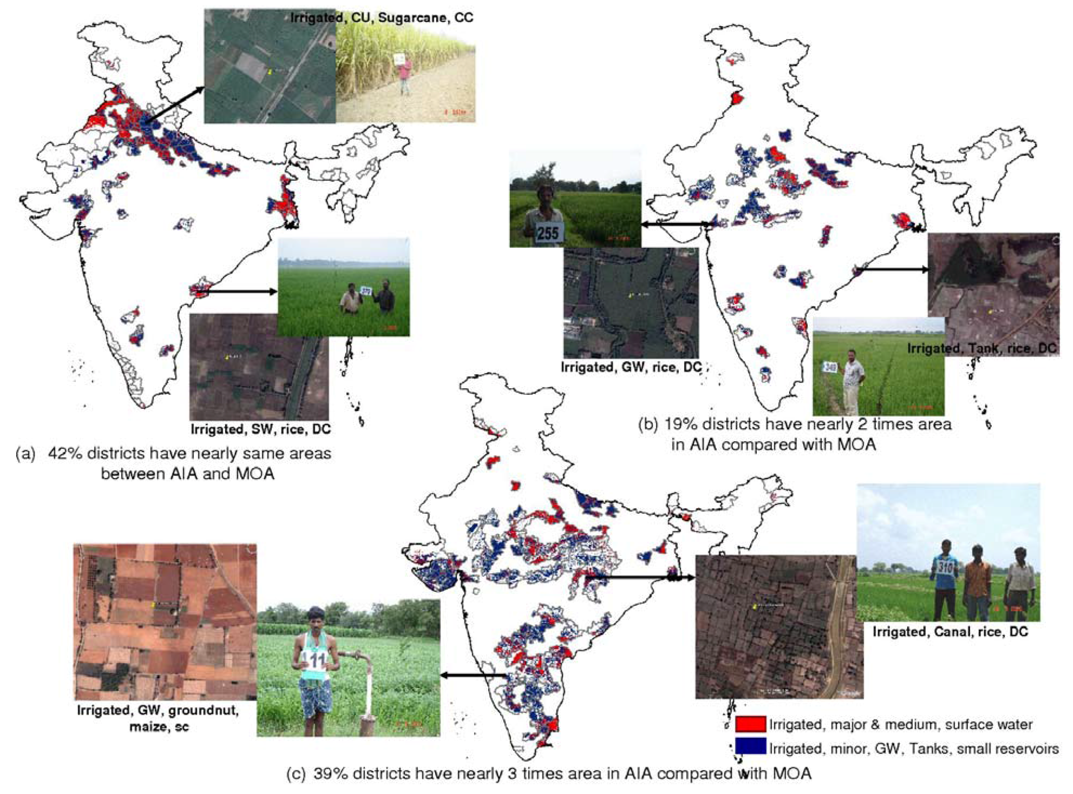
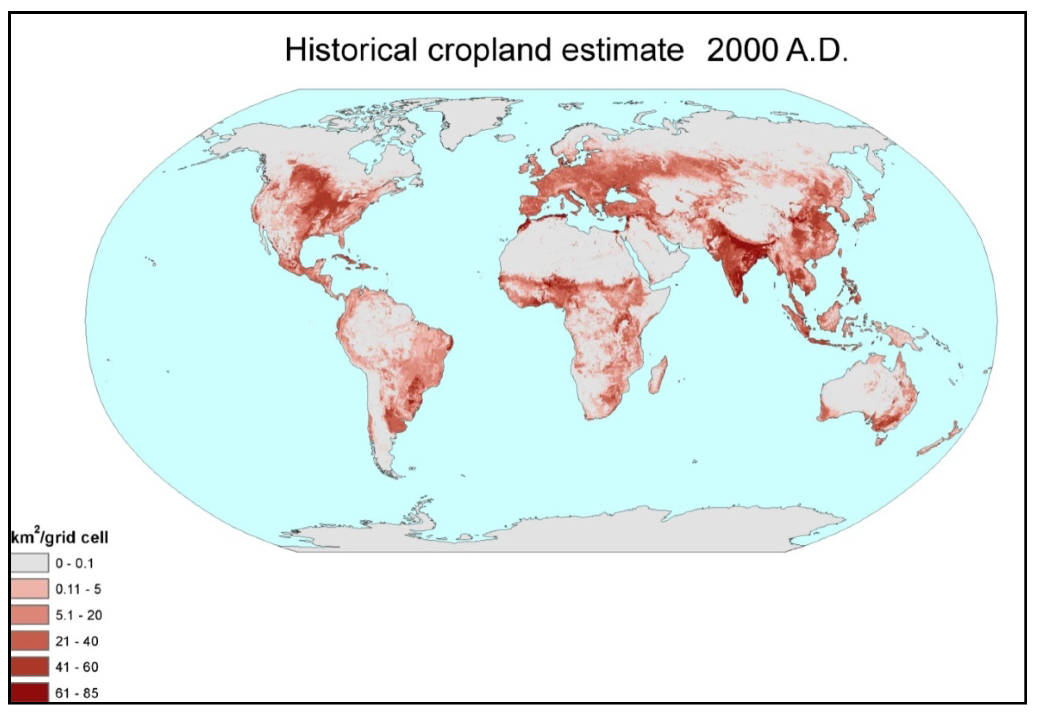
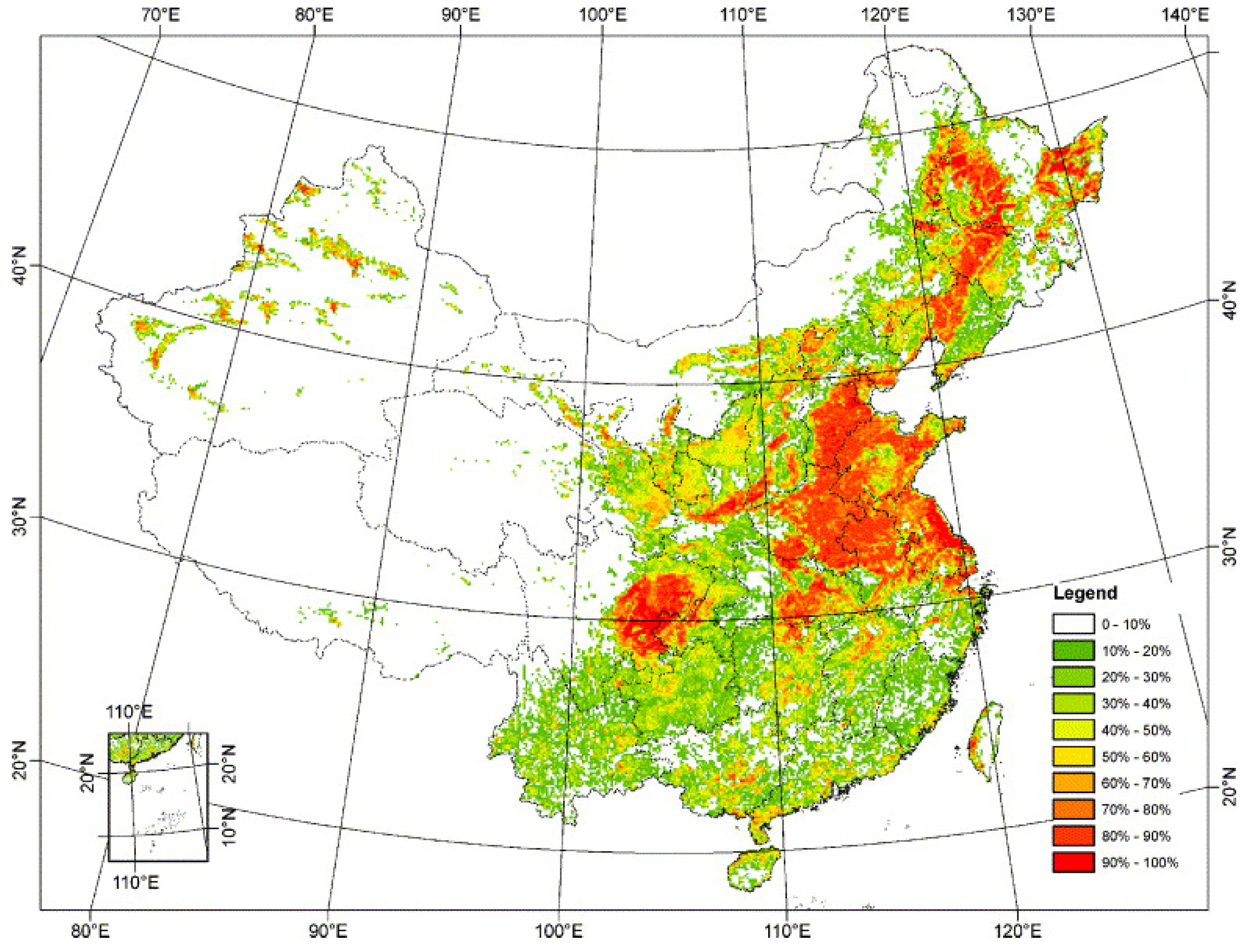
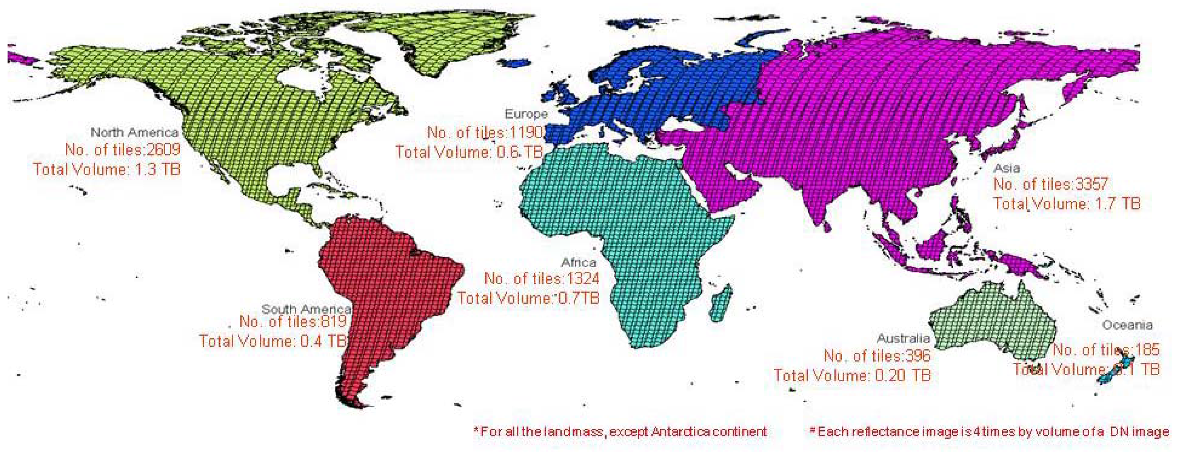
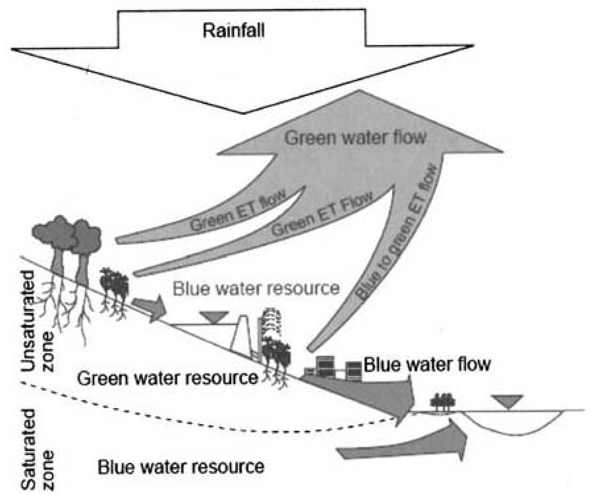
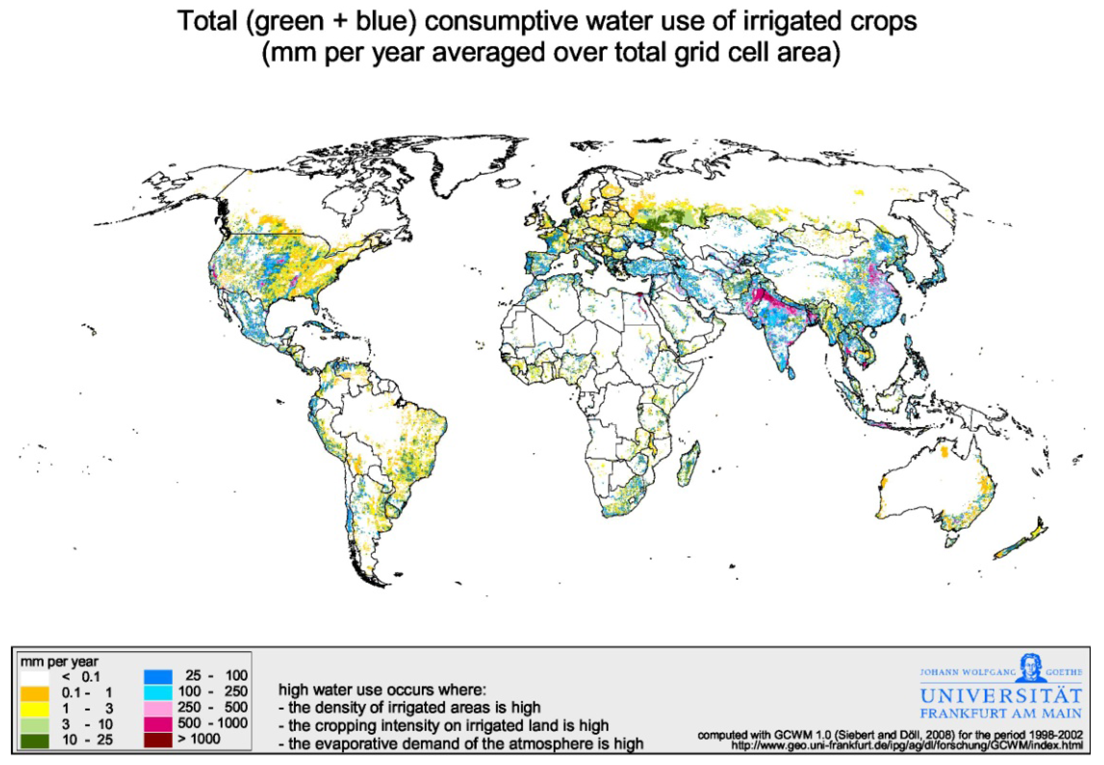
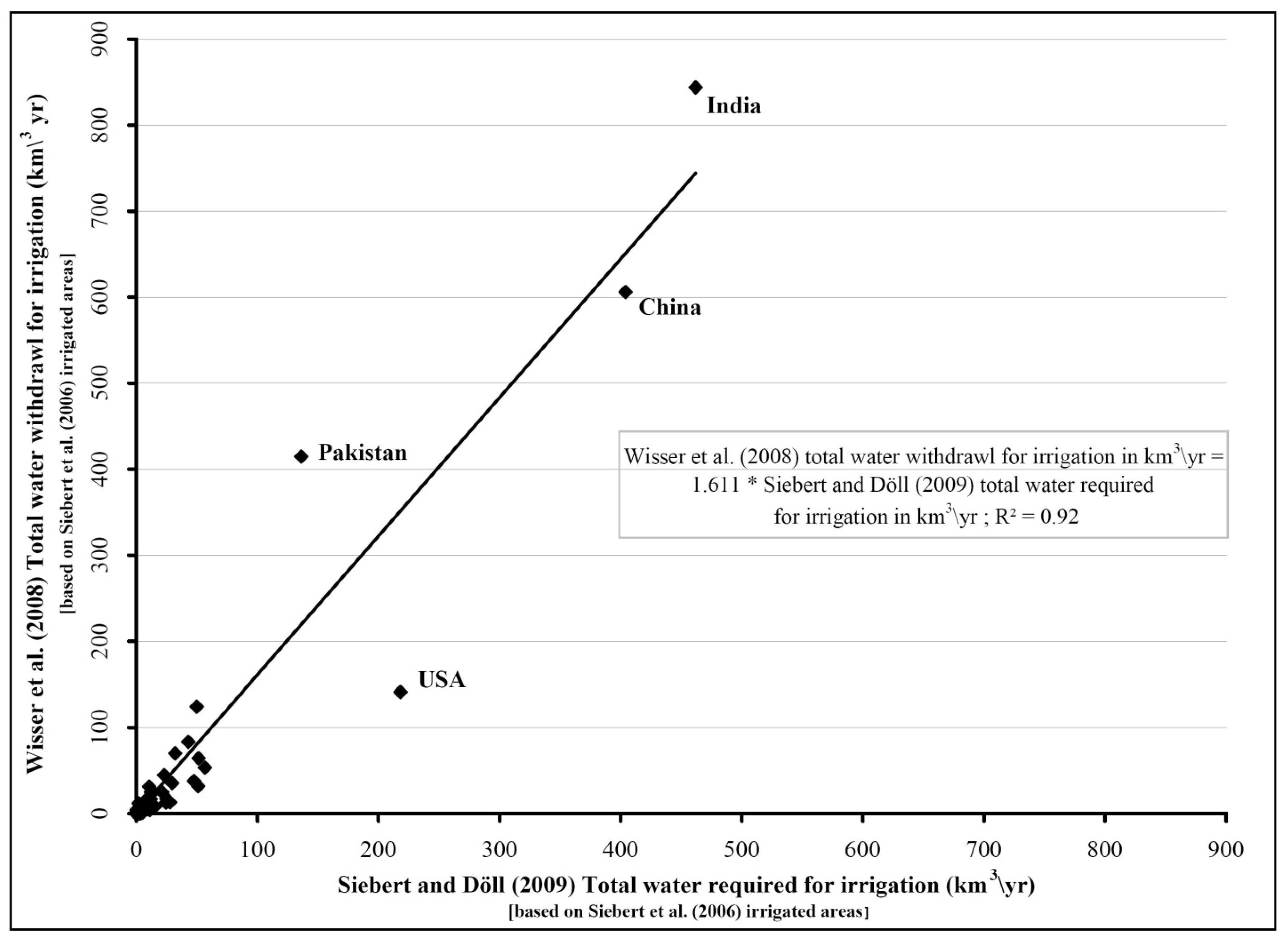
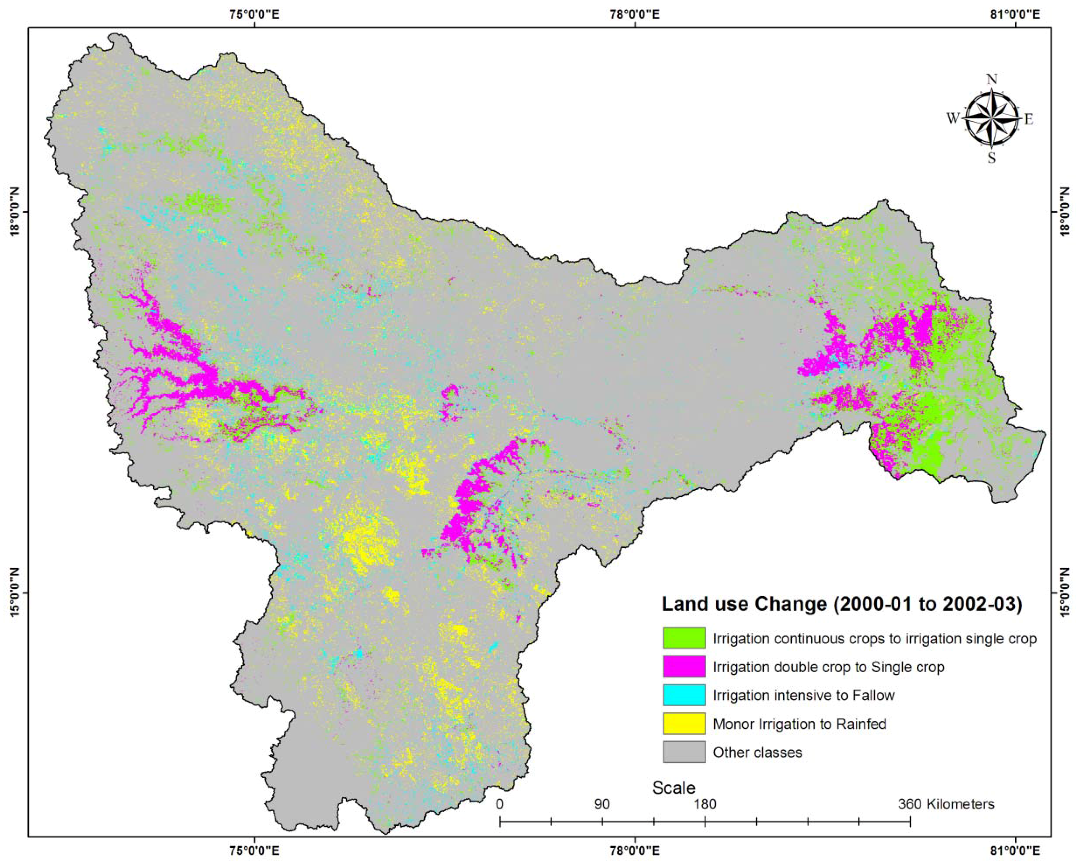Acknowledgements and Disclaimer

Authors would like to thank a number of researchers from around the world for sharing, discussing, and reviewing data presented in tables and for sharing some of the figures. They include Navin Ramankutty (Professor, Department of Geography & Earth System Science Program, McGill University), Stefan Siebert (Senior Scientist, Institute of Crop Science and Resource Conservation (INRES), University of Bonn), Kees Klein Goldewijk (Senior Scientist, Netherlands Environmental Assessment Agency), Dominick Wisser (Research Scientist, Water Systems Analysis Group. University of New Hampshire), Malin Falkenmark (Professor, SIWI and Stockholm Resilience Center), and Arjen Y. Hoekstra (Professor, Scientific Director, and Creator of the water footprint concept). The opinions expressed in the paper are those of the authors and not those of the Institutes they represent. The opinions are not endorsed by the U.S. Government.

References

Thenkabail, P.S.; Lyon, G.J.; Turral, H.; Biradar, C.M. Remote Sensing of Global Croplands for Food Security; CRC Press-Taylor and Francis Group: Boca Raton, London, UK, 2009; p. 556. [Google Scholar]
Thenkabail, P.S.; Biradar, C.M.; Noojipady, P.; Dheeravath, V.; Li, Y.J.; Velpuri, M.; Gumma, M.; Reddy, G.P.O.; Turral, H.; Cai, X.L.; Vithanage, J.; Schull, M.; Dutta, R. Global irrigated area map (GIAM), derived from remote sensing, for the end of the last millennium. Int. J. Remote Sens. 2009, 30, 3679–3733. [Google Scholar] [CrossRef]
Thenkabail, P.S.; Dheeravath, V.; Biradar, C.M.; Gangalakunta, O.P.; Noojipady, P.; Gurappa, C.; Velpuri, M.; Gumma, M.; Li, Y. Irrigated area maps and statistics of India using remote sensing and national statistics. Remote Sens. 2009, 1, 50–67. [Google Scholar] [CrossRef]
Hussain, I.; Hanjra, M.A. Does irrigation water matter for rural poverty alleviation? evidence from South and South-East Asia. Water Policy 2003, 5, 429–442. [Google Scholar]
Hussain, I.; Hanjra, M.A. Irrigation and poverty alleviation: review of the empirical evidence. Irrig. Drain. 2004, 53, 1–5. [Google Scholar] [CrossRef]
Hanjra, M.A.; Gichuki, F. Investments in agricultural water management for poverty reduction in Africa: case studies of Limpopo, Nile, and Volta river basins. Nat. Resour. Forum. 2008, 32, 185–202. [Google Scholar] [CrossRef]
FAO. In Food Outlook: Outlook Global Market Analysis; FAO: Rome, Italy, 2009.
Narayanamoorthy, A. Deceleration in agricultural growth: technology fatigue or policy fatigue? Econ. Polit. Weekly 2007, 2375–2379. [Google Scholar]
UNDP. Human Development Report 2007/2008: Fighting climate change: Human solidarity in a divided world; United Nations: New York, NY, USA, 2008. [Google Scholar]
Bindraban, P.S.; Bulte, E.H.; Conijn, S.G. Can large-scale biofuel production be sustained by 2020? Agri. Sys. 2009, 101, 197–199. [Google Scholar] [CrossRef]
Khan, S.; Hanjra, M.A. Sustainable land and water management policies and practices: a pathway to environmental sustainability in large irrigation systems. Land Degrad. Develop. 2008, 19, 469–487. [Google Scholar] [CrossRef]
Molden, D. Water responses to urbanization. Paddy Water Environ. (Special Issue Water Transfers). 2007, 5, 207–209. [Google Scholar] [CrossRef]
Jiang, Y. China's water scarcity. J. Environ. Manag. 2009, 90, 3185–3196. [Google Scholar] [CrossRef] [PubMed]
Khan, S.; Hanjra, M.A. Footprints of water and energy inputs in food production – Global perspectives. Food Policy 2009, 34, 130–140. [Google Scholar] [CrossRef]
Flavin, C.; Gardner, G. China, India, and the New World Order Chapter 1 in State of the World 2006; The World Watch Institute: Washington, DC, USA, 2006. [Google Scholar]
Funk, C.; Brown, M. Declining global per capita agricultural production and warming oceans threaten food security. Food Sec. 2009. [Google Scholar] [CrossRef]
Brown, L.R. Plan B: Rescuing a Planet Under Stress and Civilization in Trouble; Earth Policy Institute: Washington, DC, USA, 2003. [Google Scholar]
Khan, S.; Hanjra, M.A.; Mu, J. Water management and crop production for food security in China: a review. Agric. Water Manag. 2009, 96, 349–360. [Google Scholar] [CrossRef]
Wu, J.X.; Cheng, X.; Xiao, H.S.; Wang, H.; Yang, L.Z.; Ellis, E.C. Agricultural landscape change in China's Yangtze Delta, 1942–2002: A case study. Agri. Eco. Env. 2009, 129, 523–533. [Google Scholar] [CrossRef]
World Bank. Global Economic Prospects 2008: Technology Diffusion in the Developing World; The World Bank: Washington, DC, USA, 2008. [Google Scholar]
EPW, Food Security Endangered: Structural changes in global grain markets threaten India’s food security. Econ. Polit. Weekly 2008, 43, 5.
Loewenberg, S. Global food crisis looks set to continue. Lancet 2008, 372, 1209–1210. [Google Scholar] [CrossRef]
UNDP. Human Development Report 2009: Overcoming Barriers: Human Mobility and Development; United Nations: New York, NY, USA, 2009.
Pace, N.; Seal, A.; Costello, A. Food commodity derivatives: a new cause of malnutrition? Lancet 2008, 371, 1648–1650. [Google Scholar] [CrossRef]
Hanjra, M.A.; Ferede, T.; Gutta, D.G. Pathways to breaking the poverty trap in Ethiopia: Investments in agricultural water, education, and markets. Agric. Water Manag. 2009, 96, 1596–1604. [Google Scholar] [CrossRef]
Stoate, C.; Báldi, A.; Beja, P.; Boatman, N.D.; Herzon, I.; van Doorn, A.; de Snoo, G.R.; Rakosy, L.; Ramwell, C. Ecological impacts of early 21st century agricultural change in Europe—A review. J. Environ. Manag. 2009. [Google Scholar] [CrossRef] [PubMed]
Tan, Z.; Liu, S.; Tieszen, L.L.; Tachie-Obeng, E. Simulated dynamics of carbon stocks driven by changes in land use, management and climate in a tropical moist ecosystem of Ghana. Agric. Ecosyst. Environ. 2009, 130, 171–176. [Google Scholar] [CrossRef]
Lal, R. Soils and world food security. Soil Tillage Res. 2009, 102, 1–4. [Google Scholar] [CrossRef]
Lal, R. Carbon sequestration. Phil. Trans. R. Soc. B 2008, 363, 815–830. [Google Scholar] [CrossRef] [PubMed]
Thomson, A.M.; Izaurralde, R.C.; Smith, S.J.; Clarke, L.E. Integrated estimates of global terrestrial carbon sequestration. Glob. Environ. Change A 2008, 18, 192–203. [Google Scholar] [CrossRef]
Zou, J.; Liu, S.; Qin, Y.; Pan, G.; Zhu, D. Sewage irrigation increased methane and nitrous oxide emissions from rice paddies in southeast China. Glob. Environ. Change A 2009, 129, 516–522. [Google Scholar] [CrossRef]
Maraseni, T.M.; Mushtaq, S.M.; Maroulis, J. Greenhouse gas emissions from rice farming inputs: a cross-country assessment. J. Agric. Sci. 2009, 147. [Google Scholar] [CrossRef]
USEPA. Global Anthropogenic Non-CO2 Greenhouse Gas Emissions: 1990–2002; Office of Atmospheric Programs, USEPA: Washington, DC, USA, 2006.
Gleick, P.H. Global freshwater resources: soft-path solutions for the 21st century. Science 2003, 302, 1524–1528. [Google Scholar] [CrossRef] [PubMed]
Teixeira, A.H.d.C.; Bastiaanssen, W.G.M.; Ahmad, M.D.; Bos, M.G. Reviewing SEBAL input parameters for assessing evapotranspiration and water productivity for the Low-Middle São Francisco River basin, Brazil: Part B: Application to the regional scale. Agric. Forest Meteorol. 2009, 149, 477–490. [Google Scholar] [CrossRef]
Evenson, R.E.; Gollin, D. Assessing the impact of the Green Revolution 1960 to 2000. Science 2003, 300, 758–762. [Google Scholar] [CrossRef] [PubMed]
Hanjra, M.A.; Ferede, T.; Gutta, D.G. Reducing poverty in sub-Saharan Africa through investments in water and other priorities. Agric. Water Manag. 2009, 96, 1062–1070. [Google Scholar] [CrossRef]
Molden, D.; Oweis, T.; Steduto, P.; Bindraban, P.; Hanjra, M.A.; Kijne, J. Improving agricultural water productivity: Between optimism and caution. Agric. Water Manag. 2009. [Google Scholar] [CrossRef]
Hanjra, M.A.; Thenkabail, P. World water and food security under climate change and carbon trading: perspectives, pathways, opportunities and challenges for remote sensing applications. Remote Sens 2010. In Press. [Google Scholar]
Ramankutty, N.; Evan, A.T.; Monfreda, C.; Foley, J.A. Farming the planet: 1. Geographic distribution of global agricultural lands in the year 2000. Global Biogeochem. Cycles 2008, 22. [Google Scholar] [CrossRef]
Portmann, F.; Siebert, S.; Döll, P. MIRCA2000 – Global monthly irrigated and rainfed crop areas around the year 2000: a new high-resolution data set for agricultural and hydrological modelling. Global Biogeochem. Cycles 2009. 2008GB0003435. [Google Scholar] [CrossRef]
Goldewijk, K.; Beusen, A.; de Vos, M.; van Drecht, G. Holocene = Anthropocene ? The HYDE Database for Integrated Global Change Research over the Past 12,000 Years. The Holocene; Netherlands Environmental Assessment Agency: The Nethernalds, 2009.
Loveland, T.R.; Reed, B.C.; Brown, J.F.; Ohlen, D.O.; Zhu, Z.; Yang, L. Development of a global land cover characteristics database and IGBP DISCover from 1 km AVHRR data. Int. J. Remote Sens. 2000, 21, 1303–1330. [Google Scholar] [CrossRef]
Bartholome, E.; Belward, A.S. GLC2000: A new approach to global land cover mapping from Earth observation data. Int. J. Remote Sens. 2005, 26, 1959–1977. [Google Scholar] [CrossRef]
DeFries, R.; Hansen, M.; Townshend, J.R.G.; Janetos, A.C.; Loveland, T.R. Continuous Fields 1 Km Tree Cover; NASA: College Park, MD, USA, 2000.
DeFries, R.; Hansen, M.; Townsend, J.G.R.; Sohlberg, R. Global land cover classifications at 8 km resolution: the use of training data derived from Landsat imagery in decision tree classifiers. Int. J. Remote Sens. 1998, 19, 3141–3168. [Google Scholar] [CrossRef]
DeFries, R.; Hansen, M.; Townshend, J. Global discrimination of land cover types from metrics derived from AVHRR Pathfinder data. Remote Sens. Environ. 1995, 54, 209–222. [Google Scholar] [CrossRef]
Ramankutty, N.; Foley, J.A. Characterizing patterns of global land use: An analysis of global croplands data. Global Biogeochem. Cycles 1998, 12, 667–685. [Google Scholar] [CrossRef]
Siebert, S.; Döll, P. Quantifying blue and green virtual water contents in global crop production as well as potential production losses without irrigation. J. Hydrol. 2009. [Google Scholar] [CrossRef]
Goldewijk, K.K. Estimating Global land use change over the past 300 years: the HYDE Database. Global Biogeochem. Cycles 2001, 152, 417–433. [Google Scholar] [CrossRef]
Foley, J.A.; DeFries, R.; Asner, G.P.; Barford, C.; Bonan, G.; Carpenter, S.R.; Chapin, F.S.; Coe, M.T.; Daily, G.C.; Gibbs, H.K.; Helkowski, J.H.; Holloway, T.; Howard, E.A.; Kucharik, C.J.; Monfreda, C.; Patz, J.A.; Prentice, I.C.; Ramankutty, N.; Snyder, P.K. Global consequences of land use. Science 2005, 309, 570–574. [Google Scholar] [CrossRef] [PubMed]
Siebert, S.; Hoogeveen, J.; Frenken, K. Irrigation in Africa, Europe and Latin America—Update of the Digital Global Map of Irrigation Areas to Version 4; Institute of Physical Geography, University of Frankfurt: Frankfurt am Main, Rome, Italy, 2006. [Google Scholar]
Thenkabail, P.S.; Gangadhara Rao, P.; Biggs, T.; Krishna, M.; Turral, H. Spectral matching techniques to determine historical land use/land cover (LULC) irrigated areas using time-series AVHRR Pathfinder Datasets in the Krishna River Basin, India. Photogramm. Eng. Remote Sens. 2007, 73, 1029–1040. [Google Scholar]
Thenkabail, P.S.; Schull, M.; Turral, H. Ganges and Indus River Basin Land Use/Land Cover (LULC) and irrigated area mapping using Continuous Streams of MODIS Data. Remote Sens. Environ. 2005, 95, 317–341. [Google Scholar] [CrossRef]
Khan, S.; Triaq, R.; Yuanlai, C.; Blackwell, J. Can irrigation be sustainable? Agric. Water Manag. 2006, 80, 87–99. [Google Scholar] [CrossRef]
Khan, S.; Tariq, R.; Hanjra, M.A.; Zirilli, J. Water markets and soil salinity nexus: Can minimum irrigation intensities address the issue? Agric. Water Manag. 2009, 96, 493–503. [Google Scholar] [CrossRef]
Thenkabail, P.S.; Biradar, C.M.; Noojipady, P.; Cai, X.L.; Dheeravath, V.; Li, Y.J.; Velpuri, M.; Gumma, M.; Pandey, S. Sub-pixel irrigated area calculation methods. Sensors 2007, 7, 2519–2538. [Google Scholar] [CrossRef] [Green Version]
Liu, J.; Liu, M.; Tian, H.; Zhuang, D.; Zhang, Z.; Zhang, W.; Tang, X.; Deng, X. Spatial and temporal patterns of China's cropland during 1990 2000: An analysis based on Landsat TM data. Remote Sens. Environ. 2005, 98, 442–456. [Google Scholar] [CrossRef]
MoWR. Ministry of Water Resources, 3rd Census of Minor Irrigation Schemes (2000–01); Ministry of Water Resources, Govt. of India: New Delhi, India, 2005.
Endersbee, L.A. A Voyage of Discovery: A History of Ideas About the Earth, With a New Understanding of the Global Resources of Water and Petroleum, and the Problems of Climate Change; Frankston: Victoria, Australia, 2005. [Google Scholar]
Shah, T.; Ul Hassan, M.; Khattak, M.Z; Banerjee, P.S.; Singh, O.P.; Ur Rehman, S. Is irrigation water free? A reality check in the Indo-Gangetic Basin. World Dev. 2009. [Google Scholar] [CrossRef]
Shah, T.; Singh, O.P.; Mukherji, A. Some aspects of South Asia's groundwater irrigation economy: analyses from a survey in India, Pakistan, Nepal Terai and Bangladesh. Hydrogeol. J. 2006, 14, 286–309. [Google Scholar] [CrossRef]
Dheeravath, V.; Thenkabail, P.S.; Chandrakantha, G.; Noojipady, P.; Biradar, C.B.; Gumma, M.; Reddy, G.P.O.; Velpuri, M. Irrigated areas of India derived using MODIS 500 m data for years 2001–2003. ISPRS J. Photogramm. Eng. Remote Sens. 2009. In press. [Google Scholar]
Narayanamoorthy, A. Tank irrigation in India: a time series analysis. Water Policy 2007, 9, 193–216. [Google Scholar] [CrossRef]
Nickum, J.E. Irrigated area figures as bureaucratic construction of knowledge: the case of China. Water Res. Dev. 2003, 19, 249–262. [Google Scholar] [CrossRef]
Mu, J.; Khan, S.; Hanjra, M.A.; Wang, H. A food security approach to analyse irrigation efficiency improvement demands at the country level. Irrig. Drain. 2008, 58, 1–16. [Google Scholar] [CrossRef]
Hongyun, H.; Liange, Z. Chinese agricultural water resource utilization: problems and challenges. Water Policy 2007, 9, 11–28. [Google Scholar] [CrossRef]
MOA. Agricultural Statistics at a Glance; Government of India: New Dehli, India, 2008.
Dheeravath, V.; Thenkabail, P.S.; Chandrakantha, G.; Noojipady, P.; Biradar, C.B.; Turral, H.; Gumma, M.; Reddy, G.P.O.; Velpuri, M. Irrigated areas of India derived using MODIS 500 m data for years 2001–2003. ISPRS J. Photogramm. Remote Sens. http://dx.doi.org/10.1016/j.isprsjprs.2009.08.004. (In press. Corrected proof available online 22 September, 2009.).
Doraiswamy, P.C.; Hatfield, J.L.; Jackson, T.J.; Akhmedov, B.; Prueger, J.; Stern, A. Crop condition and yield simulations using Landsat and MODIS. Remote Sens. Environ. 2004, 92, 548–559. [Google Scholar] [CrossRef]
Ellis, E.C.; Wang, H.; Xiao, H.S.; Peng, K.; Liu, X. P.; Li, S.C.; Ouyang, H.; Cheng, X.; Yang, L.Z. Measuring long-term ecological changes in densely populated landscapes using current and historical high resolution imagery. Remote Sens. Environ. 2006, 100, 457–473. [Google Scholar] [CrossRef]
Seo, S.N. Is an integrated farm more resilient against climate change? A micro-econometric analysis of portfolio diversification in African agriculture. Food Policy 2009. [Google Scholar] [CrossRef]
Ozdogan, M.; Gutman, G. A new methodology to map irrigated areas using multi-temporal MODIS and ancillary data: An application example in the continental US. Remote Sens. Environ. 2008, 112, 3520–3537. [Google Scholar] [CrossRef]
NRI. National Resources Inventory. A statistical Survey of Land Use and Natural Resource Conditions and Trends on U.S. non-Federal lands; United States Department of Agriculture, Natural Resources Conservation Service: New Hampshire, NH, USA, 1997.
Velpuri, M.; Thenkabail, P.S.; Gumma, M.K.; Biradar, C.B.; Dheeravath, V.; Noojipady, P.; Yuanjie, L. Influence of resolution or scale in irrigated area mapping and area estimations. Photogramm. Eng. Remote Sens. (PE&RS) 2009, in press. [Google Scholar]
Ozdogan, M.; Woodcock, C.E. Resolution dependent errors in remote sensing of cultivated areas. Remote Sens. Environ. 2006, 103, 203–217. [Google Scholar] [CrossRef]
Tucker, C.J.; Grant, D.M.; Dykstra, J.D. NASA’s Global Orthorectified Landsat Dataset. Photogramm. Eng. Remote Sens. 2005, 70, 313–322. [Google Scholar] [CrossRef]
ERMapper. In ERMapper 7.3; software package; USA, 2007.
Biradar, C.M.; Thenkabail, P.S.; Noojipady, P.; Yuanjie, L.; Dheeravath, V.; Velpuri, M.; Turral, H.; Gumma, M. K.; Reddy, O.G.P.; Xueliang, L.C.; Schull, M.A.; Alankara, R.D.; Gunasinghe, S.; Mohideen, S.; Xiao, X. A global map of rainfed cropland areas (GMRCA) at the end of last millennium using remote sensing. Int. J. Appl. Earth Obs. Geoinf. 2009, 11, 114–129. [Google Scholar] [CrossRef]
Wardlow, B.D.; Egbert, S.L. Large-area crop mapping using time-series MODIS 250 m NDVI data: An assessment for the U.S. Central Great Plains. Remote Sens. Environ. 2008, 112, 1096–1116. [Google Scholar] [CrossRef]
Wardlow, B.D.; Egbert, S.L.; Kastens, J.H. Analysis of time-series MODIS 250 m vegetation index data for crop classification in the U.S. Central Great Plains. Remote Sens. Environ. 2007, 108, 290–310. [Google Scholar] [CrossRef]
Wardlow, B.D.; Kastens, J.H.; Egbert, S.L. Using USDA crop progress data for the evaluation of greenup onset date calculated from MODIS 250-meter data. Photogramm. Eng. Remote Sens. 2006, 72, 1225–1234. [Google Scholar] [CrossRef]
Xiao, X.; Boles, S.; Frolking, S.; Li, C.; Babu, J.Y.; Salas, W. Mapping paddy rice agriculture in South and Southeast Asia using multi-temporal MODIS images. Remote Sens. Environ. 2006, 100, 95–113. [Google Scholar] [CrossRef]
Friedl, M.A.; McIver, D.K.; Hodges, J.C.F.; Zhang, X.Y.; Muchoney, D.; Strahler, A.H. Global land cover mapping from MODIS: Algorithms and early results. Remote Sens. Environ. 2002, 83, 287–302. [Google Scholar] [CrossRef]
Hansen, M.C.; DeFries, R.S.; Townshend, J.R.G.; Sohlberg, R.; Dimiceli, C.; Carroll, M. Towards an operational MODIS continuous field of percent tree cover algorithm: examples using AVHRR and MODIS data. Remote Sens. Environ. 2002, 83, 303–319. [Google Scholar] [CrossRef]
Crist, E.P.; Cicone, R.C. Application of the tasseled cap concept to simulated Thematic Mapper data. Photogramm. Eng. Remote Sens. 1984, 50, 343–352. [Google Scholar]
Masek, J.G.; Huang, C.; Wolfe, R.; Cohen, W.; Hall, F.; Kutler, J.; Nelson, P. North American forest disturbance mapped from a decadal Landsat record. Remote Sens. Environ. 2008, 112, 2914–2926. [Google Scholar] [CrossRef]
Cohen, W.B.; Goward, S.N. Landsat's role in ecological applications of remote sensing. BioScience 2004, 54, 535–545. [Google Scholar] [CrossRef]
Gordon, L.J.; Peterson, G.D.; Bennett, E. Agricultural modifications of hydrological flows create ecological surprises. Trends Ecol. Evolut. 2008, 23, 211–219. [Google Scholar] [CrossRef] [PubMed]
Jewitt, G. Integrating blue and green water flows for water resources management and planning. Physc. Chem. Earth, Parts A/B/C 2006, 31, 753–762. [Google Scholar] [CrossRef]
Falkenmark, M.; Rockström, J. The New Blue and Green Water paradigm: Breaking new ground for water resources planning and management. J. Water Res. Plan. Manag. 2006, 132, 1–15. [Google Scholar] [CrossRef]
Savenije, H.H.G. The importance of interception and why we should delete the term evapotranspiration from our vocabulary. Hydrological Processes 2004, 18, 1507–1511. [Google Scholar] [CrossRef]
Rockström, J.; Falkenmark, M.; Karlberg, L.; Hoff, H.; Rost, S.; Gerten, D. Future water availability for global food production: The potential of green water for increasing resilience to global change. Water Resour. Res. 2009, 45. [Google Scholar] [CrossRef]
Portmann, F.; Siebert, S.; Bauer, C.; Döll, P. Global Data Set of Monthly Growing Areas of 26 Irrigated Crops; University of Frankfurt: Frankfurt am Main, Germany, 2008. [Google Scholar]
Postel, S. Water for food production: Will there be enough in 2025? BioScience 1998, 48, 629–637. [Google Scholar] [CrossRef]
Wisser, D.; Frolking, S.; Douglas, E.M.; Fekete, B.M.; Vorosmarty, C.J.; Schumann, A.H. Global irrigation water demand: Variability and uncertainties arising from agricultural and climate data sets. Geophys. Res. Lett. 2008, 35. [Google Scholar] [CrossRef]
Siebert, S.; Döll, P. The Global Crop Water Model (GCWM): Documentation and First Results for Irrigated Crops; University of Frankfurt: Frankfurt am Main, Germany, 2008. [Google Scholar]
Wichelns, D. The role of 'virtual water' in efforts to achieve food security and other national goals, with an example from Egypt. Agric. Water Manag. 2001, 49, 131–151. [Google Scholar] [CrossRef]
Wichelns, D. The policy relevance of virtual water can be enhanced by considering comparative advantages. Agric. Water Manag. 2004, 66, 49–63. [Google Scholar] [CrossRef]
Wichelns, D. The virtual water metaphor enhances policy discussions regarding scarce resources. Water Int. 2005, 30, 428–437. [Google Scholar] [CrossRef]
Allan, J.A. Virtual water: a strategic resource. Global solutions to regional deficits. Groundwater 1998, 36, 545–546. [Google Scholar] [CrossRef]
Ramirez-Vallejo, J.; Rogers, P. Virtual water flows and trade liberalization. Water Sci. Technol. 2004, 49, 25–32. [Google Scholar] [PubMed]
Hoekstra, A.Y. The Water Footprint of Food; Twente Water Centre, University of Twente: The Netherlands, 2008; Available online: http://www.waterfootprint.org/Reports/Hoekstra-2008-WaterfootprintFood.pdf (Accessed on 4 January 2010).
Gerbens-Leenes, P.W.; Hoekstra, A.Y.; van der Meer, T. The water footprint of energy from biomass: A quantitative assessment and consequences of an increasing share of bio-energy in energy supply. Ecol. Econ. 2008. [Google Scholar] [CrossRef]
van Hofwegen, P. How Important is the Virtual Water Debate in Ensuring Food Security? World Water Council: The Hauge, The Netherlands, 2008. [Google Scholar]
Kumar, M.D.; Singh, O.P. Virtual water in global food and water policy making: Is there a need for rethinking? Water Resour. Manag. 2005, 19, 759–789. [Google Scholar] [CrossRef]
Hoekstra, A.Y.; Chapagain, A.K. Water footprints of nations: water use by people as a function of their consumption pattern. Water Resour. Manag. 2007, 21, 35–48. [Google Scholar] [CrossRef]
Hoekstra, A.Y.; Hung, P.Q. Globalisation of water resources: international virtual water flows in relation to crop trade. Glob. Environ. Change A 2005, 15, 45–56. [Google Scholar] [CrossRef]
Bringezu, S.; Schütz, H.; Arnold, K.; Merten, F.; Kabasci, S.; Borelbach, P.; Michels, C.; Reinhardt, G.A.; Rettenmaier, N. Global implications of biomass and biofuel use in Germany - Recent trends and future scenarios for domestic and foreign agricultural land use and resulting GHG emissions. J. Cleaner Prod. 2009. In press. [Google Scholar] [CrossRef]
Johnson, M.; Hazell, P.; Gulati, A. The role of intermediate factor markets in Asia's Green Revolution: lessons for Africa. Am. J. Agric. Econ. 2003, 85, 1211–1216. [Google Scholar] [CrossRef]
Binswanger, H.P.; Khandker, S.R.; Rosenzweig, M.W. How infrastructure and financial institutions affect agricultural output and investment in India. J. Devel. Econ. 1993, 41, 337–366. [Google Scholar] [CrossRef]
Gumma, M.K.; Thenkabail, P.S.; Gangadhara Rao, T.P.; Nalan, S.A.; Velpuri, M.N.; Biradar, C. Agriculture Cropland Change Response to Water availability using Spectral Matching Techniques in the Krishna River Basin (India) (Review). Int. J. Remote Sens. 2009, TRES-PAP-2009, 0162. [Google Scholar]
Rajagopalan, B.; Nowak, K.; Prairie, J.; Hoerling, M.; Harding, B.; Barsugli, J.; Ray, A.; Udall, B. Water supply risk on the Colorado River: Can management mitigate? Water Resour. Res. 2009, 45. [Google Scholar] [CrossRef]
Kirby, M.; Mainuddin, M. Water and agricultural productivity in the Lower Mekong Basin: trends and future prospects. Water Int. 2009, 34, 134–143. [Google Scholar] [CrossRef]
Connell, D.; Grafton, R.Q. Planning for water security in the Murray-Darling Basin. Public Policy 2008, 3, 67–86. [Google Scholar]
Qureshi, M.E.; Shi, T.; Qureshi, S.E.; Proctor, W. Removing barriers to facilitate efficient water markets in the Murray-Darling Basin of Australia. Agric. Water Manag. 2009, 96, 1641–1651. [Google Scholar] [CrossRef]
Guo, R.; Lin, Z.; Mo, X.; Yang, C. Responses of crop yield and water use efficiency to climate change in the North China Plain. Agric. Water Manag. 2009. [Google Scholar] [CrossRef]
Malthus, T.R. An Essay on the Principle of Population. CHAPTER 1; St. Paul's Churchyard: London, UK, 1798; p. 13. [Google Scholar]
McIntyre, B.D. International Assessment of Agricultural Knowledge, Science and Technology for Development (IAASTD); Global Report: Oxford, UK, April, 2008. [Google Scholar]
Hossain, M.; Janaiah, A.; Otsuka, K. Is the productivity impact of the Green Revolution in rice vanishing? Econ. Polit. Weekly 2005, 5595–9600. [Google Scholar]
Turral, H.; Svendsen, M.; Faures, J. Investing in irrigation: Reviewing the past and looking to the future. Agric. Water Manag. 2009. [Google Scholar] [CrossRef]
Vinnari, M.; Tapio, P. Future images of meat consumption in 2030. Futures 2009. [Google Scholar] [CrossRef]
Gordon, L.J.; Finlayson, C.M.; Falkenmark, M. Managing water in agriculture for food production and other ecosystem services. Agric. Water Manag. 2009, 97. [Google Scholar] [CrossRef]
Foley, J.A.; Monfreda, C.; Ramankutty, N.; Zaks, D. Our share of the planetary pie. PNAS 2007, 104, 12585–12586. [Google Scholar] [CrossRef] [PubMed]
Lal, R.; Pimentel, D. Biofuels from crop residues. Soil Tillage Res. 2009, 93, 237–238. [Google Scholar] [CrossRef]
Gibbs, H.K.; Johnston, M.; Foley, J.A.; Holloway, T.; Monfreda, C.; Ramankutty, N.; Zaks, D. Carbon payback times for crop-based biofuel expansion in the tropics: the effects of changing yield and technology. Environ. Res. Lett. 2008, 034001. [Google Scholar] [CrossRef]
Searchinger, T.; Heimlich, R.; Houghton, R.A.; Dong, F.; Elobeid, A.; Fabiosa, J.; Tokgoz, S.; Hayes, D.; Yu, T.H. Use of U.S. Croplands for Biofuels Increases Greenhouse Gases Through Emissions from Land-Use Change. Science 2008, 319, 1238–1240. [Google Scholar] [CrossRef] [PubMed]
Platonov, A.; Thenkabail, P.S.; Biradar, C.; Cai, X.; Gumma, M.; Dheeravath, V.; Cohen, Y.; Alchanatis, V.; Goldshlager, N.; Ben-Dor, E.; Vithanage, J.; Manthrithilake, H.; Kendjabaev, S. Water Productivity Mapping (WPM) using Landsat ETM+ Data for the Irrigated Croplands of the Syrdarya River Basin in Central Asia. Sensors 2008, 8, 8156–8180. [Google Scholar] [CrossRef] [Green Version]
Hussain, I.; Mudasser, M.; Hanjra, M.A.; Amrasinghe, U.; Molden, D. Improving Wheat Productivity in Pakistan: Econometric Analysis Using Panel Data from Chaj in the Upper Indus Basin. Water Int. 2004, 29, 189–200. [Google Scholar] [CrossRef]
Kantor, L.; Lipton, K.; Manchester, A.; Oliveira, V. Estimating and addressing America’s food losses. Food Review 1997, Jan.–Apr., 2–12. [Google Scholar]
Shiva, V. Stolen Harvest: the Highjacking of the Global Food Supply; South End Press and Zed Books: Boston, MA, USA, 2000. [Google Scholar]
Shiva, V. The future of food: countering globalisation and recolonisation of Indian agriculture. Futures 2004, 36, 715–732. [Google Scholar] [CrossRef]
Gleick, P.H.; Cooley, H. Statistics compiled by Gleick P.H. and Cooley H. of the Pacific Institute 2009. Statistics available online at: http://www.worldwater.org/data.html (Accessed on 4January 2010).
United Nations Food and Agricultural Organization's Aquastat (FAO AQUASTAT). Available online at: http://www.fao.org/NR/WATER/AQUASTAT/water_use/index.stm (Accessed on 4 January 2010).

© 2010 by the authors; licensee Molecular Diversity Preservation International, Basel, Switzerland. This article is an open-access article distributed under the terms and conditions of the Creative Commons Attribution license (http://creativecommons.org/licenses/by/3.0/).

Share and Cite

MDPI and ACS Style

Thenkabail, P.S.; Hanjra, M.A.; Dheeravath, V.; Gumma, M. A Holistic View of Global Croplands and Their Water Use for Ensuring Global Food Security in the 21st Century through Advanced Remote Sensing and Non-remote Sensing Approaches. Remote Sens. 2010, 2, 211-261. https://doi.org/10.3390/rs2010211

AMA Style

Thenkabail PS, Hanjra MA, Dheeravath V, Gumma M. A Holistic View of Global Croplands and Their Water Use for Ensuring Global Food Security in the 21st Century through Advanced Remote Sensing and Non-remote Sensing Approaches. Remote Sensing. 2010; 2(1):211-261. https://doi.org/10.3390/rs2010211

Chicago/Turabian Style

Thenkabail, Prasad S., Munir A. Hanjra, Venkateswarlu Dheeravath, and Muralikrishna Gumma. 2010. "A Holistic View of Global Croplands and Their Water Use for Ensuring Global Food Security in the 21st Century through Advanced Remote Sensing and Non-remote Sensing Approaches" Remote Sensing 2, no. 1: 211-261. https://doi.org/10.3390/rs2010211

Article Menu

A Holistic View of Global Croplands and Their Water Use for Ensuring Global Food Security in the 21st Century through Advanced Remote Sensing and Non-remote Sensing Approaches

Abstract

1. Introduction

2. Global Croplands

3. Uncertainties in Cropland Area Estimates

4. Cropland Areas at Finer Resolutions

5. Way Forward in Cropland Mapping

6. Global Cropland Water Requirements and Withdrawal: Blue, Green, and White Water

7. Virtual Water Use

8. Croplands, Crop Water Availability, Climate Change, and Food Security

9. A New Paradigm for Future Food Security

10. Conclusions and Policy Implications

Acknowledgements and Disclaimer

References

Share and Cite

Article Metrics

Article Access Statistics

Further Information

Guidelines

MDPI Initiatives

Follow MDPI