Article

Classification of Defoliated Trees Using Tree-Level Airborne Laser Scanning Data Combined with Aerial Images

1
Department of Forest Sciences, University of Helsinki, Helsinki, Finland
2
Finnish Geodetic Institute, FI-02431, Masala, Finland
3
Norwegian Forest and Landscape Institute, Norway
*
Author to whom correspondence should be addressed.
Remote Sens. 2010, 2(12), 2665-2679; https://doi.org/10.3390/rs2122665
Submission received: 12 October 2010 / Revised: 18 November 2010 / Accepted: 22 November 2010 / Published: 26 November 2010

Abstract

:
Climate change and rising temperatures have been observed to be related to the increase of forest insect damage in the boreal zone. The common pine sawfly (Diprion pini L.) (Hymenoptera, Diprionidae) is regarded as a significant threat to boreal pine forests. Defoliation by D. pini can cause severe growth loss and tree mortality in Scots pine (Pinus sylvestris L.) (Pinaceae). In this study, logistic LASSO regression, Random Forest (RF) and Most Similar Neighbor method (MSN) were investigated for predicting the defoliation level of individual Scots pines using the features derived from airborne laser scanning (ALS) data and aerial images. Classification accuracies from 83.7% (kappa 0.67) to 88.1% (kappa 0.76) were obtained depending on the method. The most accurate result was produced using RF with a combination of data from the two sensors, while the accuracies when using ALS and image features separately were 80.7% and 87.4%, respectively. Evidently, the combination of ALS and aerial images in detecting needle losses is capable of providing satisfactory estimates for individual trees.

1. Introduction

The world’s climate has experienced dramatic changes over the past decades causing, among other things, rising temperatures across the globe [1]. The present changes have already resulted in numerous effects on species’ distribution and phenology, leading to damage by insect pests in managed forests (e.g., [2,3,4]). The rate of change, e.g., in mean annual temperature, is higher at higher latitudes, such as in Nordic countries. Biological invasions and climate change are two of the components of global change comprising the greatest environmental challenges of today [5]. Predicting changes in the distribution of and damage from pest organisms has become a topical issue in the field of forest research.
Some forest insects, formerly regarded as harmless species, have now altered their pest status and are causing serious damage in Finland [6,7]. Economic losses from needle defoliators can be considerable, approximately EUR 300–1000 per hectare, depending on the intensity of needle loss and number of years with high population densities. It can require over a decade for a tree to fully recover after a 1–3 year outbreak [8].
Diprion pini is a univoltine species in Scandinavia that consumes all the needle age-classes of Scots pine in August and September. This could lead to a total defoliation of host trees in the peak phase of population dynamics [9,10]. Mature and maturing trees have the highest defoliation risk [10,11], and trees of that age have the highest economic value. A massive outbreak by D. pini occurred in dry and dryish pine forests in central Finland between 1997 and 2001, covering 500,000 ha [6]. The outbreak reached easternmost Finland in 1999 (Ilomantsi district), and the chronic sawfly densities have fluctuated in the area ever since.
There is an increased need for rapid assessment methods of forests affected by such hazardous events [12]. The symptoms of forest damage by insects are in many cases visible from far distances. Some types of forest damage such as crown discoloration, defoliation and dieback are even more visible from a bird’s eye view than from the ground. In particular, a better assessment of the dispersion and range extension pattern can be based on remote sensing (RS) data. RS can produce data for large, inaccessible forest lands quickly and at a much lower cost than ground surveys [13,14].
The recent development of RS technologies, particularly airborne laser scanning (ALS), has provided new tools for forest inventory and monitoring. With its ability to directly measure forest structure, including canopy height and crown dimensions, ALS is increasingly used for forest inventories at different levels. Previous studies have shown that ALS data can be used to estimate a variety of forest inventory attributes including tree, plot and stand level estimates for tree height [15,16,17,18], biomass [19,20,21], volume [22,23,24], basal area [20,25,26] and tree species [21,27,28,29,30].
ALS is also a promising method for monitoring forest hazards and defoliation, because of its ability to derive vegetation structure properties. The capability of ALS to map defoliation has been demonstrated for a pine sawfly attack in Norway [31]. ALS data were acquired both before and after the insect attack, and the defoliation was derived from the change in penetration rate and Leaf Area Index (LAI). Further studies have indicated that it might be possible to derive defoliation data even without having repeated ALS acquisitions [32], and that different types of disturbances to some extent can be distinguished based on the type of ALS penetration through the forest canopy [33]. In those studies the defoliation mapping was carried out with a spatial resolution of 10 × 10 m, 20 × 20 m or for forest stands. However, an attempt to derive single tree defoliation data was not successful [34].
The aim of the present study was to test the accuracy of needle loss detection, determined by features extracted from ALS and image data. We propose the hypothesis that the distribution of the laser returns of a defoliated tree differs from that of a healthy tree estimated by LASSO, RF and MSN methods. Classification accuracy (%) and kappa values were calculated for accuracy evaluation.

2. Material and Methods

2.1. Study Area
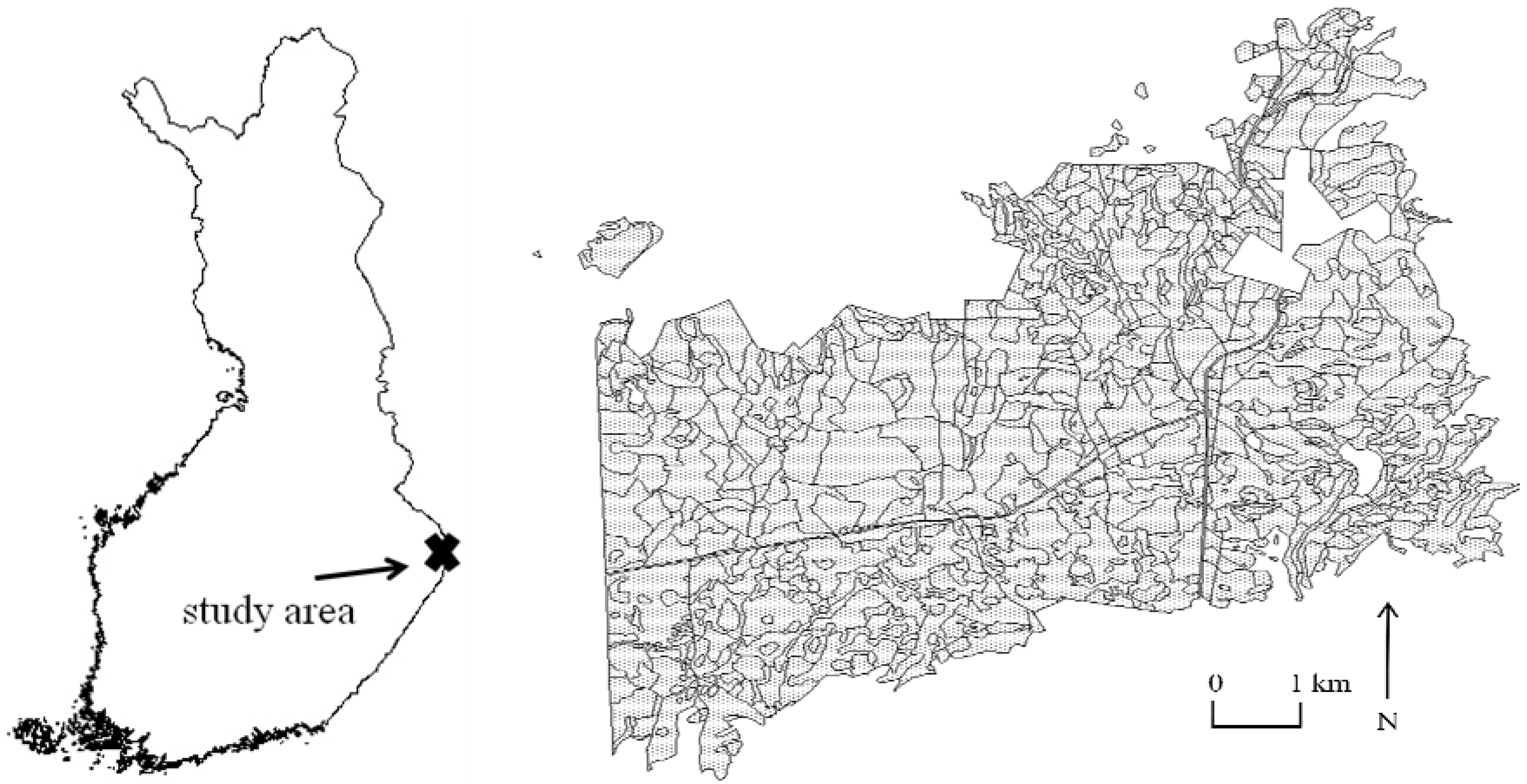
The current study was performed in Eastern Finland, in the Ilomantsi district (62°53′N, 30°54′E) (Figure 1). The study area, covering 34.5 km2, was located in a region where D. pini has caused considerable damage in an area of 10,000 ha during the past 10 years. The field inventory was carried out in May and June 2009. The forest stands in the study area were mainly pure pine stands growing on dry to dryish sandy soil sites. The majority of the stands were young or middle-aged forests having an average age of 53 years and a diameter of 14.7 cm.
Figure 1. Location (left) and map with forest compartments (right) of the study area in Ilomantsi district.
Remotesensing 02 02665 g001

2.2. Field Data

The visual assessment of defoliation intensity was carried out simultaneously with tree-wise measurements in the field sampling plots. The sampling plot centers were located in the field with a Trimble Pro XH (Trimble Navigation Ltd., Sunnyvale, CA, U.S.), which can reach up to 30-cm precision. Differential post processing was applied. The individual trees were located by measuring the distance and angle from north of a tree from the plot center. The intensity of defoliation of a single tree was visually estimated from different directions from the tree according to Eichhorn [35]. In the method, the amount of the needles of a tree under investigation is compared to a reference tree with full healthy foliage growing on the same site type. An accuracy of 10% was used in the estimation of needle loss. The defoliation percentage of 20% was determined as a threshold of severe needle loss, due to annual growth losses of 40–50% in the forthcoming years, after a consumption of 20% of the total needle biomass by D. pini [36].
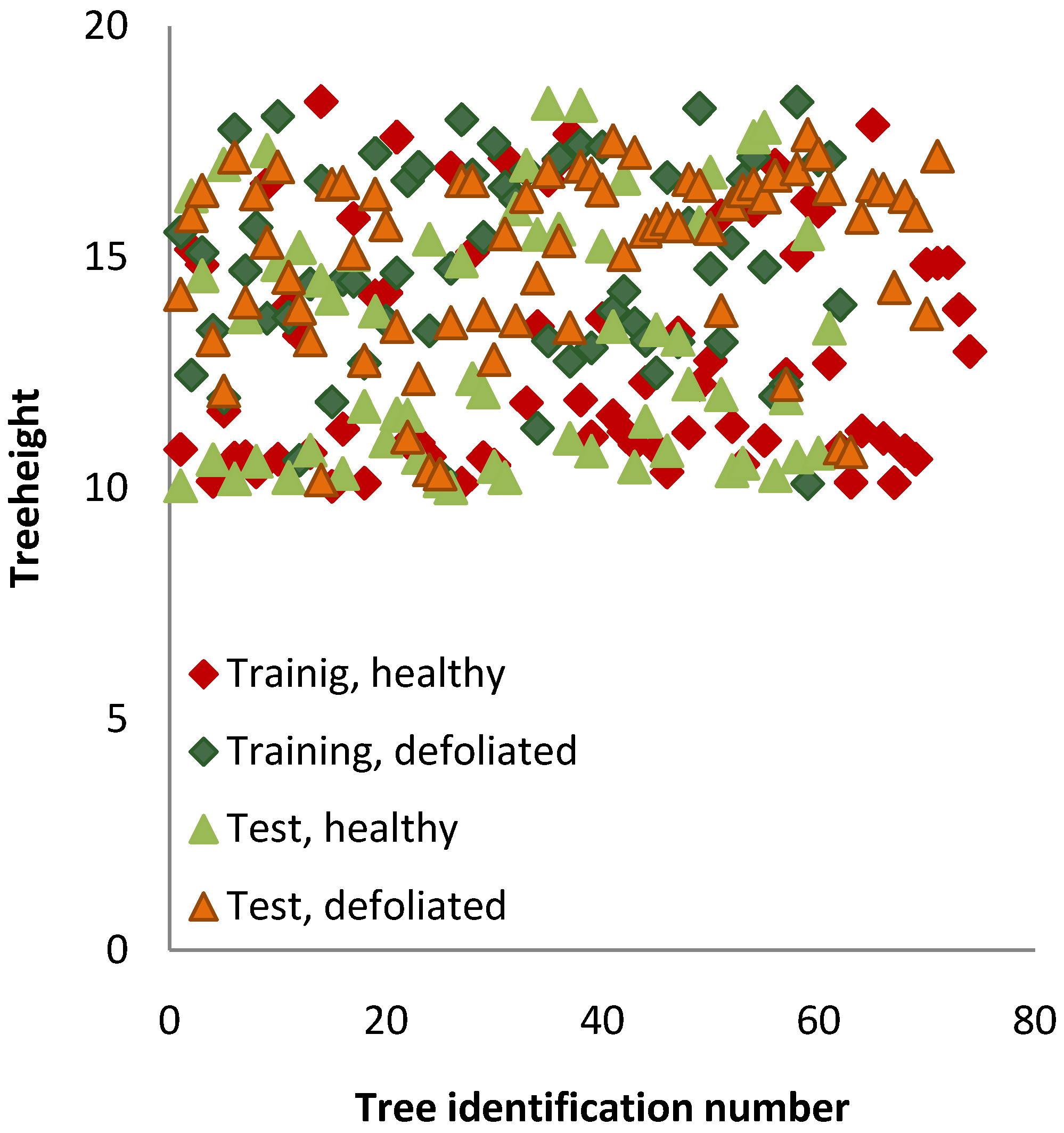
A sample of 271 single Scots pines detected from the ALS data was chosen for the analysis. Half of the pines suffered from severe needle loss and the other half were healthy (Table 1). The data were randomly divided into training data (136 trees) and test data (135 trees). Size, age and canopy strata affect the defoliation level of a tree. In the study area, the taller and older trees in dominant canopy strata were typically more defoliated than younger ones. To achieve reliable results, the aforementioned effects needed to be eliminated. Therefore, the analysis was limited to the same size and age categories of trees from the dominant canopy strata in both classes. Size distribution was based on tree height (Figure 2). The trees in healthy classes had a defoliation level 10% or less and in defoliated classes 20% or more.
Table 1. Statistics of trees in defoliated and healthy categories, where d is the laser diameter at breast height and h is the laser height of a tree.
ndmeandmindmaxdsdhmeanhminhmaxhsd
TrainingDefoliated6219.312.824.23.014.810.118.42.2
TrainingHealthy7416.712.724.23.513.010.018.42.5
TestDefoliated7419.712.923.22.715.110.217.72.0
TestHealthy6117.012.624.23.613.210.018.32.6
Figure 2. Plotted heights of healthy and defoliated trees. The x axis presents the identification number of a tree in class i and the y axis presents the height of a tree in class I, where i is a defoliation class in data set.
Remotesensing 02 02665 g002

2.3. Remote Sensing Material

The ALS data were acquired in July 2008 with a Leica ALS50-II SN058 laser scanner (Leica Geosystem AG, Heerbrugg, Switzerland). The flying altitude was 500 m at a speed of 80 knots, with a field of view of 30 degrees, pulse rate of 150 kHz, scan rate of 52 Hz and size of the laser footprint on the ground of 0.11 m. The density of the returned pulses within the field plots was approximately 20 pulses per m2. Aerial images were taken with a Vexcel Ultracam digital camera (Vexcel Corporation, Boulder, CO, U.S.). The flying altitude was 5,850 m and the resolution of the images was 50 cm. It was assumed that there were no significant changes in defoliation status between the acquisition of ALS data and the field measurements due to finalized elongation of current shoots of pine trees.
ALS data were classified into ground or non-ground points using the standard TerraScan approach as explained by Axelsson [37]. A digital terrain model was created using classified ground points. Laser heights above ground (normalized height or canopy height) were calculated by subtracting the ground elevation from corresponding laser measurements. Heights greater than 2 m were considered as vegetation returns, and only these were used for tree feature extraction.

2.4. Tree Detection and Feature Extraction

A raster canopy height model (CHM) was created from normalized data for individual tree detection and crown segmentation. Single tree segmentations were performed on the CHM images using a minimum curvature-based region detector [38]. During the segmentation processes, the tree crown shape and location of individual trees were determined. The procedure consisted of the following steps:
(1).
The CHM was smoothed with a Gaussian filter to remove small variations on the crown surface. The degree of smoothness was determined by the value of standard deviation (Gaussian scale) and kernel size of the filter.
(2).
Minimum curvatures were calculated. Minimum curvature is one of the principal curvatures. For a surface like CHM, a higher value of minimum curvature describes the tree top.
(3).
The smoothed CHM image was then scaled based on the computed minimum curvature resulting in a smoothed yet contrast-stretched image.
(4).
Local maxima were then searched for in a given neighborhood. These were considered as tree tops and used as markers in the following marker-controlled watershed transformation for tree crown delineations.
Each segment was considered to present a single tree crown. Laser returns falling within each individual tree segment were extracted and the canopy heights of these returns were used to derive the tree features. Spectral features near-infrared (NIR), red (R) and green (G) were extracted from the aerial images using a window size of 4 × 4 pixels, representing the average crown size (determined from individual tree detection (ITD) results; Table 2).
Table 2. Features extracted from ALS data and aerial images for individual trees.
FeatureDescription
HmaxMaximum laser height
HmeanArithmetic mean of laser heights
HstdStandard deviation of heights
CHCrown height
CACrown area as a convex hull
CVCrown volume as a convex hull in 3D
HP10-90Heights 0th–90th percentile
DS10-90Percentage of returns below 10–90% of total height
MaxDMaximum crown diameter when crown was considered as an ellipse
PonlyPercentage of only returns
PfirstPercentage of first returns
PintermedianPercentage of intermedian returns
PlastPercentage of last returns
NIRSpectral value of NIR band from aerial image
GSpectral value of green band from aerial image
RSpectral value of red band from aerial image

2.5. Classification Methods

2.5.1. Logistic LASSO Regression

The logistic regression is a basic method for classifying phenomena to two different classes. The LASSO is a shrinkage and selection method for linear regression. It minimizes the usual sum of squared errors, with a bound on the sum of the absolute values of the coefficients. The LASSO method is described in further detail in Tibshirani [39]. The probability of the defoliation class of the trees was modeled with multiple logistic LASSO regression, using the function glm in the R statistical package [40]. Logistic regression is commonly used in modeling the probability of occurrence of an event. In logistic regression, logit transformation is used to make the relationship between the response probability and the explanatory variables linear. The multiple logistic regression model is expressed as follows:
logit(p) = ln[p/(1 − p)] = β0 + β1 × 1 + β2x2 +….+ βnxn
where p is the probability that an event will occur and x1…xn are the variables explaining the probability. The predicted probabilities are calculated by reverting back to the original scale:
p = exp(logit(p))/[1 + exp(logit(p))].

2.5.2. RF

The Random Forests algorithm, proposed by Breiman [41], is a nonparametric estimation approach. The method is composed of a set of regression trees that are constructed from bootstrapped training data. The bootstrapped data consist in general of sets of samples taken randomly with replacement from the original training set. A regression tree is built for each of the bootstrap sets. Random forests are created by averaging over trees. A regression tree is a sequence of rules that split the feature space into partitions having similar values to the response variable. A method based on a classification and regression tree is usually adopted to generate regression trees. At each node of a regression tree, data are split until the leaf nodes contain fewer samples than some preselected value, or the sum of squares of distances to the mean value of the respective group is less than the threshold. RF is described and used for the estimation of tree variables (e.g., in [38]). The R yaimpute library [42] was used in calculations.

2.5.3. MSN

A common nonparametric estimation method that is applied in operational forest management planning ALS inventory in Finland is k-Most-Similar-Neighbor (k-MSN). In k-MSN, the similarity is based on canonical correlations and the Mahalanobis distance [43]. The benefit of the k-MSN method is that the similarity measurement can be solved analytically. The k-MSN method is the same as MSN except that it takes the k nearest observations (in feature space) into account. The R yaImpute library [42] was applied in the MSN estimations.
Before MSN estimation, automatic feature selection was carried out using the simple genetic algorithm (GA) presented by Goldberg [44] and implemented in the R GALGO library [45]. The GA process starts by generating an initial population of strings (chromosomes or genomes) that consists of separate features (genes). The strings evolve during a user-defined number of iterations (generations). The evolution includes the following two operations: (1) Selecting strings for mating using a user-defined objective criterion (better if more copies are in the mating pool); (2) Letting the strings in the mating pool swap parts (crossing over), causing random noise (mutations) in the offspring (children) and passing the resulting strings onto the next generation. GA was used with promising results previously in ALS feature selection for nonparametric estimation [46].

3. Results

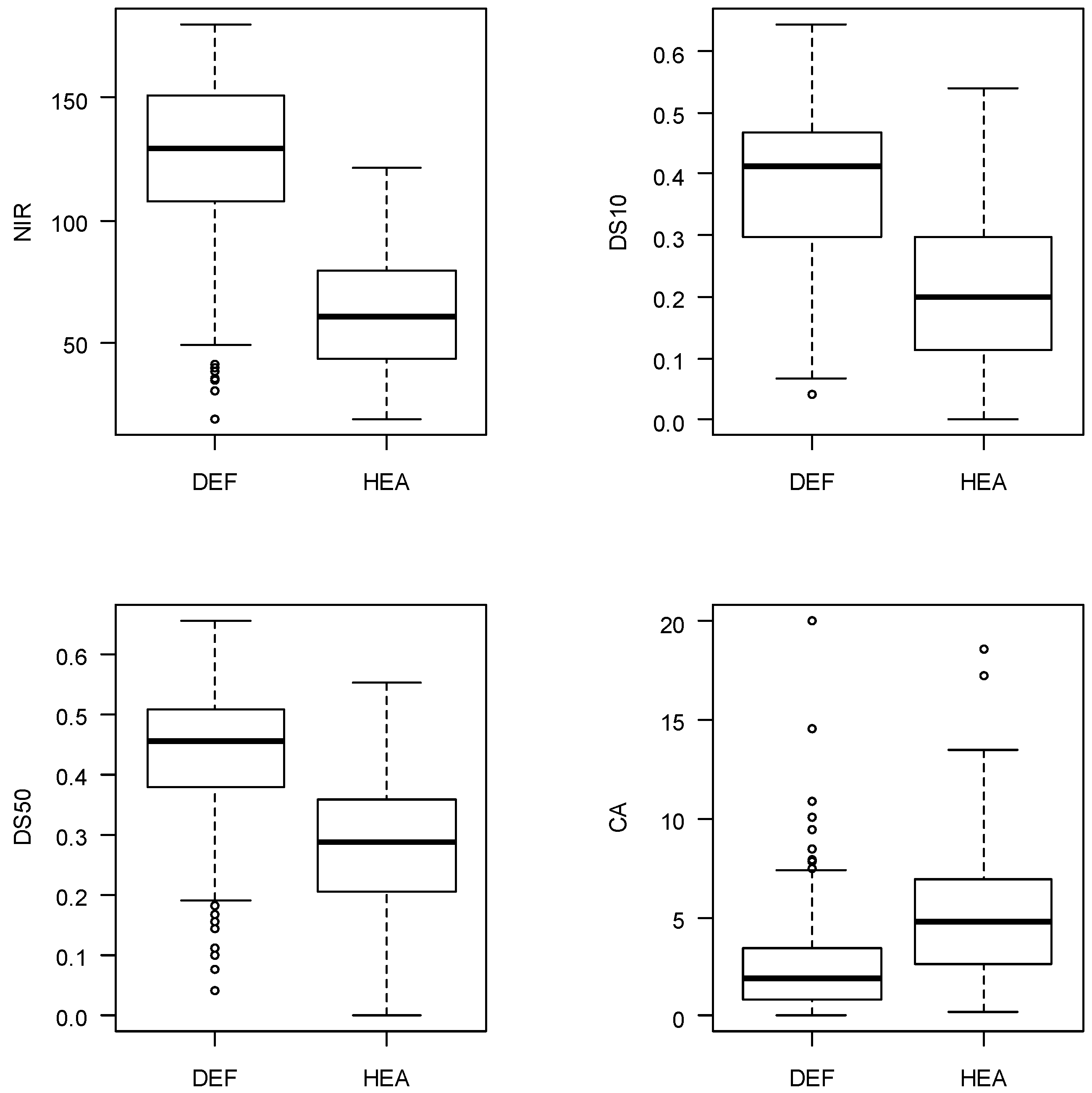
It can be seen that distributions of ALS and spectral features of the aerial photographs vary between healthy and defoliated trees (Figure 3). Mean spectral values of the NIR band from aerial image show that defoliated trees are brighter than healthy ones. Furthermore, more pulses are returned from lower heights if trees are defoliated (Figure 3, DS10, DS50), and the mean crown area determined from ALS data (CA) is smaller in defoliated trees than in those which are healthy.
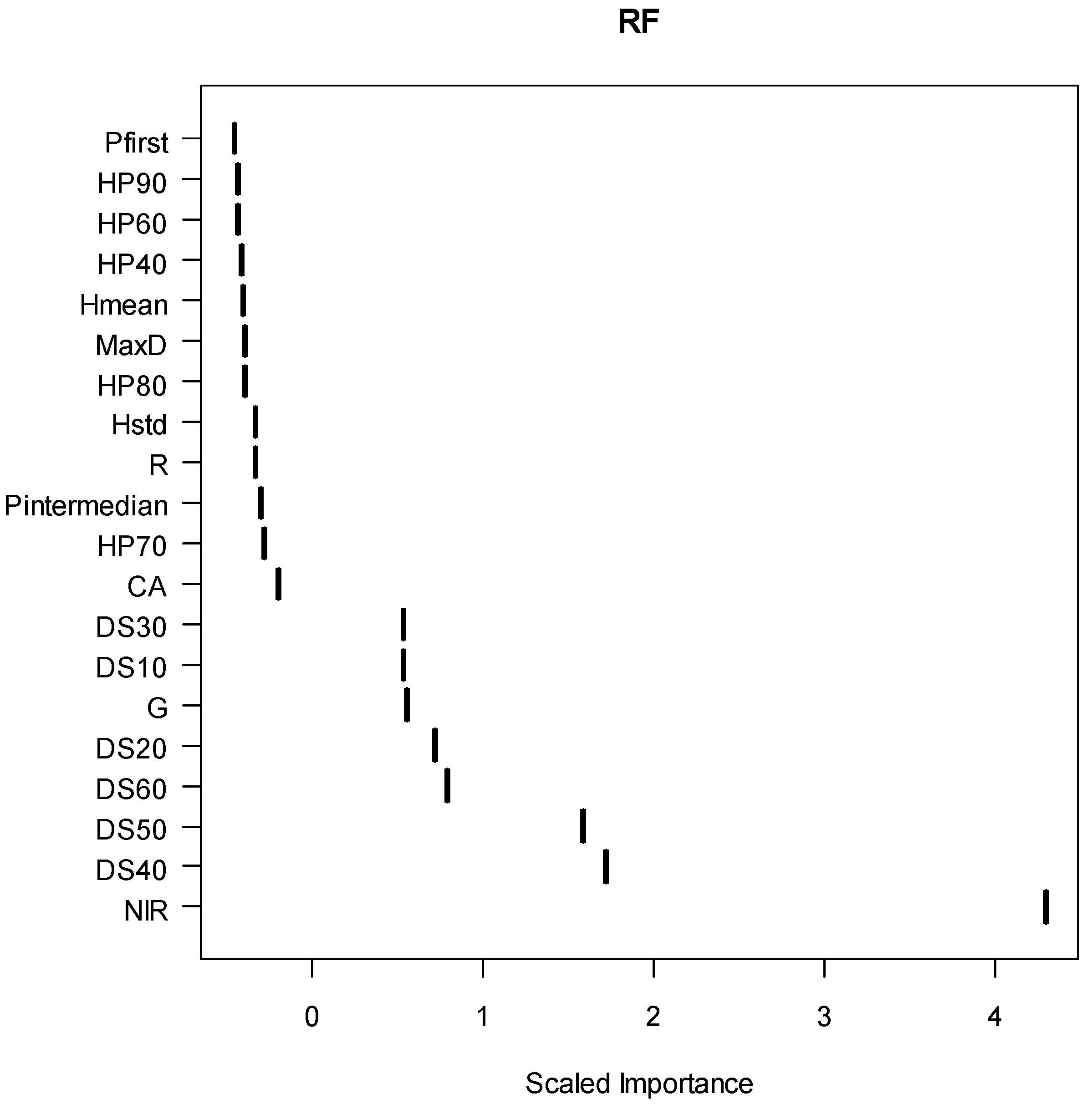
LASSO regression achieved an accuracy of 86.7% with a respective kappa value of 0.73. Selected LASSO features, such as CA, DS10, DS50, and NIR gained the highest values (Table 3). The RF method classified the defoliated trees with an accuracy of 88.1%. The respective kappa value was 0.76. The most important features used in the RF classification were NIR, DS40, DS50, DS30, DS20, DS10, DS60 and G. Figure 4 shows the relatively scaled importance of different features from RF, e.g., NIR from aerial image is over two-times more important than the ALS feature DS40, which is the second most important. Before MSN estimation, the following features were selected with GA: CA, HP70, DS50, DS60, NIR and G (Table 3). Classification accuracy using MSN was 83.7% (kappa value 0.67). The errors in classification occurred both ways in every method. There were few more defoliated trees classified to healthy group than healthy ones to defoliated group.
Figure 3. NIR, DS10, DS50 and CA features used in the classification of defoliated (DEF) and healthy (HEA) trees. Table 2 describes the features.
Remotesensing 02 02665 g003
Table 3. Selected features and parameter estimates for LASSO and MSN. Classification accuracies and kappa values for LASSO, RF and MSN are presented under the selected features. Table 2 describes the features.
Predictor LASSORFMSN
Estimate
intercept 5.6742999
CA 0.1391846
HP70
DS10 −2.375357
DS50 −4.244455
DS60
NIR −0.042489
G
Train setClassification accuracy91.20%96.30%85.30%
Kappa value0.810.910.66
Test setClassification accuracy86.7%88.1%83.7%
Kappa value0.730.760.67
With the RF method, single sensor data was also tested for classification. When only laser derived features were used, classification accuracy of 80.7% was achieved. The respective accuracy with aerial photographs only was 87.4%.
Figure 4. Importance of features in classifying defoliated trees using RF. Higher values indicate features that are more important to the classification. For feature descriptions, see Table 2.
Remotesensing 02 02665 g004

4. Discussion

In the present study, statistical ALS features combined with spectral features of aerial images were tested in the classification of defoliation of individual trees. LASSO, RF and MSN methods were applied to classification of defoliation into severely defoliated and healthy trees. This kind of classification procedure enables testing the possible ability to detect severe defoliation from ALS data.
The methods (RF, LASSO and MSN) showed seemingly promising results, when applied to detecting heavy defoliation by means of ALS data. According to our knowledge, this study is the first one for detection of insect defoliation. These methods have been used in several studies in the estimation of forest characteristics other than defoliation at stand and tree level [29,30,38,47,48].
The MSN and RF were chosen for this study for the following reasons. MSN is a widely used method in Finnish forest planning and thereby has a straight linkage to practical forestry. The new applications for a method already used should be easier to adapt. In recent studies, the RF has proved to be a promising method in estimating tree- and stand wise variables. One advantage of using the RF is that no separate feature selection is needed.
The detection from single sensors was also tested. Detection using only aerial image features worked quite well. However, the result was slightly better combined with the ALS features. At the operational level, the aerial images are often acquired at the same time as ALS and the combination of both can be utilized.
Defoliation level was visually estimated using the same procedure utilized by the National Forest Inventory (NFI) of Finland [49]. However, visual interpretation could easily cause deviation in the results if the surveyors were not professionals. Naked-eye calibration is essential when two or more researchers are estimating the critical variable. Observers should also recognize a natural variation in the growth pattern of foliage biomass. In addition, prevailing conditions could also cause bias in the defoliation assessment, e.g., weather, brightness, heavy wind, high tree density, difficult terrain, etc. In this study, it was assumed that there were no significant changes in defoliation status between acquisition of ALS and field measurement due to increased diapause rate and mortality of sawflies. Temperature was exceptionally low and precipitation high during the summer months in 2008, enabling most of pine trees to finalize elongation of current shoots without a significant sawfly activity.
According to our results, it is possible to detect trees and forest stands with high defoliation intensity using combined high pulse density ALS and aerial images. This may be an important finding for detecting and mapping insect damage which is usually a rare and clustered phenomenon. It may also be meaningful auxiliary information for improving the inventory of forest damage. For example, with RS data, the stratification could be carried out by focusing on more plots in areas where pest damage could already be detected from the preliminary RS data.
To the best of our knowledge the use of ALS ITD inventory for estimating tree defoliation has not been previously investigated. However, the results of this study are in some ways comparable with those of Ilvesniemi and Karjalainen et al. [50,53]. Ilvesniemi [50] used the same Palokangas study area as was utilized here when investigating the usability of aerial photographs and Landsat TM in classifying Scots pine defoliation at plot level. The tested estimation methods were the maximum likelihood method, unsupervised classification and linear regression model. The image features used for needle loss detection were spectral and textural features and vegetation indices. The classification accuracies when using features extracted from aerial photographs varied between 38% (nine classes) and 87.3% (two classes). The best explanatory variable for needle loss was aerial image NIR channel maximum radiation (r2 = 0.69). Classification results with Landsat image features were slightly poorer than with the best aerial image feature set (accuracy between 25.4% and 88.7%). Aerial images have been applied also in other studies to detect the plot or stand wise defoliation level (see e.g., [51,52]). Haara and Nevalainen [51] studied also the tree wise detection accuracy for Norway spruce (Picea abies L.). The classification accuracy for reference data was 68.9% with four classes.
Karjalainen et al. [53] used multitemporal ERS-2 and Envisat satellite images and calculated the SAR backscattering intensities (squared amplitude) of 400 m × 400 m grid cells. These SAR features were used to estimate defoliation (same two classes as used here). The reference information on the forest health status of each grid cell was determined by a specialist in forest protection, applying the method over the last two decades. A threshold value of 20% was employed, i.e., if needle defoliation in the grid cell was estimated to be more than 20%, then the reference value for classification was set as “Heavy defoliation exists”. When 30% of the field reference was used in training and 70% for testing the model, an overall classification accuracy of 67.8% was obtained.
This study is one of the first steps towards developing an ALS- and aerial photograph-based system for monitoring changes in forest health (defoliation) in Finland. Optimally, defoliation mapping should be included in current practices; for example, it should be part of the National Forest Inventories (NFI) or operational forest management planning that will in the future be performed based on the ALS inventory. Field surveys will provide information on growing stock estimation and also more precise information about needle defoliation when needed. Then, ALS and aerial images can be applied on demand to create stem volume maps and detect status and spatial occurrence of forest defoliation. In this study, the high density ALS was utilized. The classification accuracies might have been presumably lower using low density ALS data, which is commonly used at the operational level at present. However the pulse densities are assumingly increasing in the future also in practical implementations.
Further studies will focus on testing the classification accuracy with more defoliation classes. From a practical point of view, it is most important to detect areas of severe defoliation, therefore the use of only two classes in our first tests was justified. When several defoliation classes are used, non-parametric estimation methods will also be tested. The optimal feature extraction and selection for this kind of purpose should be studied further. Further, the use of ALS intensity could improve classification accuracy.

5. Conclusions

We showed that distributions of ALS pulses and spectral features of aerial photographs vary between healthy and defoliated trees. It was possible to achieve 83.7%–88.1% (kappa values 0.67–0.76) classification accuracy for the two defoliation classes. RF provided the best results, but the difference compared to the other methods (LASSO and MSN) was not large. The difference between the best (RF) and the worst (MSN) performing method in this study was 4.4%. The accuracies of using ALS and image features separately were 80.7% and 87.4%, respectively. It seems that high pulse density ALS data combined with aerial images could be utilized when mapping and monitoring forest defoliation. However, further studies are needed with respect to using more defoliation classes and for linking developed methods to operational forest inventories.

Acknowledgements

This study was made possible by financial aid from the Maj and Tor Nessling Foundation, Foresters foundation Niemi Foundation and the Finnish Academy project Improving Forest Supply Chain by Means of Advanced Laser Measurements (L-IMPACT). We thank also Tornator Oy for the cooperation.

References

  1. IPCC 2007. Summary for policymakers. In Climate Change 2007: The Physical Science Basis; Contribution of Working Group 1 to the Fourth Assessment Report of the Intergovernmental Panel on Climate Change; Solomon, S., Qin, D., Manning, M., Chen, Z., Marquis, M., Avyret, K.B., Tignor, M., Miller, H.L., Eds.; Cambridge University Press: Cambridge, UK and New York, NY, USA, 2007. [Google Scholar]
  2. Dale, V.H.; Joyce, L.A.; McNulty, S.; Neilson, R.P.; Ayres, M.P.; Flannican, M.D.; Hanson, P.J.; Irland, L.C.; Lugo, A.E.; Peterson, C.J.; Simberloff, D.; Swanson, F.J.; Stocks, B.J.; Wotton, B.M. Climate change and forest disturbances. Biosciences 2001, 51, 723–734. [Google Scholar] [CrossRef]
  3. Evans, H.; Straw, N.; Watt, A. Climate change: Implication for insect pests. In Climate Change: Impact on UK Forests; Roadmeadow, M., Ed.; Forestry Commission Bulletin 125; Forestry Commisssion: Edinburgh, UK, 2002; pp. 99–118. [Google Scholar]
  4. Walther, G.R.; Post, E.; Convey, P.; Menzel, A.; Parmesan, C.; Beebee, T.J.C.; Fromentin, J.-M.; Hoegh-Guldberg, O.; Bairlein, F. Ecological responses to recent climate change. Nature 2002, 416, 389–395. [Google Scholar] [CrossRef] [PubMed]
  5. Logan, J.A.; Regniere, J.; Powell, J.A. Assessing the impacts of global warming on forest pest dynamics. Front. Ecol. Environ. 2003, 1, 130–137. [Google Scholar] [CrossRef]
  6. Lyytikäinen-Saarenmaa, P.; Tomppo, E. Impact of sawfly defoliation on growth of Scots pine Pinus sylvestris (Pinaceae) and associated economic losses. Bull. Entomol. Res. 2002, 92, 137–140. [Google Scholar] [CrossRef] [PubMed]
  7. De Somviele, B.; Lyytikäinen-Saarenmaa, P.; Niemelä, P. Stand edge effects on distribution and condition of Diprionid sawflies. Agr. Forest Entomol. 2007, 9, 17–30. [Google Scholar] [CrossRef]
  8. Lyytikäinen-Saarenmaa, P.; Niemelä, P.; Annila, E. Growth responses and mortality of Scots pine (Pinus sylvestris L.) after a pine sawfly outbreak. In Forest Insect Population Dynamics and Host Influences, In Proceedings of International Symposium of IUFRO, Kanazawa, Japan, September 14–19, 2003; Kamata, N., Liebhold, A.L., Quiring, D.T., Clancy, K.M., Eds.; Kanazawa University: Kanazawa, Ishikawa, Japan, 2003; pp. 81–85. [Google Scholar]
  9. Viitasaari, M.; Varama, M. Sawflies 4. Conifer sawflies (Diprionidae); Department of Agricultural and Forest Zoology Reports; University of Helsinki: Helsinki, Finland, 1987; pp. 1–79, (In Finnish with an English summary). [Google Scholar]
  10. Geri, G. The pine sawfly in central France. In Dynamics of Forest Insect Populations: Patterns, Causes, Implications; Berryman, A.A., Ed.; Plenum Press: New York, NY, USA, 1988; pp. 377–405. [Google Scholar]
  11. De Somviele, B.; Lyytikäinen-Saarenmaa, P.; Niemelä, P. Sawfly (Hym. Diprionidae) outbreaks on Scots pine: Effect of stand structure, site quality and relative tree position on defoliation intensity. Forest Ecol. Manag. 2004, 194, 305–317. [Google Scholar] [CrossRef]
  12. Lyytikäinen-Saarenmaa, P.; Holopainen, M.; Ilvesniemi, S.; Haapanen, R. Detecting pine sawfly defoliation by means of remote sensing and GIS. Forstschutz Aktuell. 2008, 44, 14–15. [Google Scholar]
  13. Ciesla, W. Remote Sensing in Forest Health Protection; USDA Forest Service Remote Sensing Applications Center: Salt Lake City; UT and Forest Health Technology Enterprise Team: Fort Collins, CO, USA, 2000.
  14. Hall, R.J.; Skakun, R.S.; Arsenault, E.J. Remotely sensed data in the mapping of insect defoliation. In Understanding Forest Disturbance and Spatial Pattern: Remote Sensing and GIS Approaches; Michael, W.A., Franklin, S.E., Eds.; CRC Press, Taylor & Francis Group: Boca Raton, FL, USA, 2007; pp. 85–111. [Google Scholar]
  15. Falkowski, M.J.; Smith, A.M.S.; Hudak, A.T.; Gessler, P.E.; Vierling, L.A.; Crookston, N.L. Automated estimation of individual conifer tree height and crown diameter via two-dimensional spatial wavelet analysis of lidar data. Can. J. Remote Sens. 2006, 32, 153–161. [Google Scholar] [CrossRef]
  16. Hyyppä, J.; Inkinen, M. Detecting and estimating attributes for single trees using laser scanner. Photogramm. J. Fin. 1999, 16, 27–42. [Google Scholar]
  17. Magnussen, S.; Eggermont, P.; LaRiccia, V.N. Recovering tree heights from airborne laser scanner data. Forest Sci. 1999, 45, 407–422. [Google Scholar]
  18. Maltamo, M.; Mustonen, K.; Hyyppä, J.; Pitkänen, J.; Yu, X. The accuracy of estimating individual tree variables with airborne laser scanning in boreal nature reserves. Can. J. Forest Res. 2004, 34, 1791–1801. [Google Scholar] [CrossRef]
  19. Bortolot, Z.; Wynne, R.H. Estimating forest biomass using small footprint LiDAR data: An individual tree-based approach that incorporates training data. ISPRS J. Photogramm. Remote Sens. 2005, 59, 342–360. [Google Scholar] [CrossRef]
  20. Lefsky, M.A.; Harding, D.; Cohen, W.B.; Parker, G.; Shugart, H.H. Surface lidar remote sensing of basal area and biomass in deciduous forests of Eastern Maryland, USA. Remote Sens. Environ 1999, 67, 83–98. [Google Scholar] [CrossRef]
  21. Van Aardt, J.A.N.; Wynne, R.H.; Scrivani, J.A. Lidar-based mapping of forest volume and biomass by taxonomic group using structurally homogenous segments. Photogramm. Eng. Remote Sensing 2008, 74, 1033–1044. [Google Scholar] [CrossRef]
  22. Hyyppä, J.; Kelle, O.; Lehikoinen, M.; Inkinen, M. A segmentation-based method to retrieve stem volume estimates from 3-D tree height models produced by laser scanners. IEEE Trans. Geosci. Remote Sens. 2001, 39, 969–975. [Google Scholar] [CrossRef]
  23. Næsset, E. Estimating timber volume of forest stands using airborne laser scanner data. Remote Sens. Environ 1997, 61, 246–253. [Google Scholar] [CrossRef]
  24. Wallerman, J.; Holmgren, J. Estimating field-plot data of forest stands using airborne laser scanning and SPOT HRG data. Remote Sens. Environ. 2007, 110, 501–508. [Google Scholar] [CrossRef]
  25. Means, J.E.; Acker, S.A.; Fitt, B.J.; Renslow, M.; Emerson, L.; Hendrix, C.J. Predicting forest stand characteristics with airborne scanning lidar. Photogramm. Eng. Remote Sensing. 2000, 66, 1367–1371. [Google Scholar]
  26. Næsset, E. Predicting forest stand characteristics with airborne scanning laser using a practical two-stage procedure and field data. Remote Sens. Environ. 2002, 80, 88–99. [Google Scholar] [CrossRef]
  27. Brandtberg, T. Classifying individual tree species under leaf-off and leaf-on conditions using airborne lidar. ISPRS J. Photogramm. Remote Sens. 2007, 61, 325–340. [Google Scholar] [CrossRef]
  28. Holmgren, J.; Persson, Å. Identifying species of individual trees using airborne laser scanner. Remote Sens. Environ. 2004, 90, 415–423. [Google Scholar] [CrossRef]
  29. Korpela, I.; Ørka, H.O.; Maltamo, M.; Tokola, T.; Hyyppä, J. Tree species classification using airborne LiDAR—Effects of stand and tree parameters, downsizing of training set, intensity normalization, and sensor type. Silva Fenn. 2010, 44, 319–339. [Google Scholar] [CrossRef]
  30. Vauhkonen, J.; Korpela, I.; Maltamo, M.; Tokola, T. Imputation of single-tree attributes using airborne laser scanning-based height, intensity and alpha shape metrics. Remote Sens. Environ. 2010, 114, 1263–1276. [Google Scholar] [CrossRef]
  31. Sohlberg, S.; Næsset, E.; Hanssen, K.H.; Christiansen, E. Mapping defoliation during a severe insect attack on Scots pine using airborne laser scanning. Remote Sens. Environ. 2006, 102, 364–376. [Google Scholar] [CrossRef]
  32. Solberg, S.; Næsset, E. Monitoring forest health by remote sensing. In Symposium on Forests in a Changing Environment—Results of 20 years ICP Forests Monitoring, Göttingen, Germany, October 25–28, 2006; Schriftenreihe der Forstlichen Fakultät Göttingen und der Nordwestdeutschen Forstlichen Versuchsanstalt: Göttingen, Germany, 2007a; pp. 99–104. [Google Scholar]
  33. Solberg, S. Mapping gap fraction, LAI and defoliation using various ALS penetration variables. Int. J. Remote Sens. 2010, 32, 1227–1244. [Google Scholar] [CrossRef]
  34. Solberg, S.; Næsset, E. Mapping defoliation with LIDAR. In ISPRS Workshop on Laser Scanning 2007 and SilviLaser 2007, Espoo, Finland, September 12–14, 2007; Volume 3/W52, pp. 379–382.
  35. Eichhorn, J. Manual on Methods and Criteria for Harmonized Sampling, Assessment, Monitoring and Analysis of the Effects of Air Pollution on Forests. Part II. Visual Assessment of Crown Condition and Submanual on Visual Assessment of Crown Condition on Intensive Monitoring Plots; United Nations Economic Commission for Europe Convention on Long-range Transboundary Air Pollution: Hamburg, Germany, 1998. [Google Scholar]
  36. Lyytikäinen-Saarenmaa, P. Unpublished data.
  37. Axelsson, P. DEM generation from laser scanner data using adaptive TIN models. In XIX ISPRS Congress, Commission I-VII, Amsterdam, The Netherlands, July 16–23, 2000; pp. 110–117.
  38. Yu, X.; Hyyppä, J.; Holopainen, M.; Vastaranta, M.; Viitala, R. Predicting individual tree attributes from airborne laser point clouds based on random forest technique. ISPRS J. Photogramm. Remote Sens. 2010. In press. [Google Scholar] [CrossRef]
  39. Tibshirani, R. Regression shrinkage and selection via the lasso. J. Royal. Statist. Soc B. 1996, 58, 267–288. [Google Scholar]
  40. R Development Core Team. R: A Language and Environment for Statistical Computing; R Foundation for Statistical Computing: Vienna, Austria, 2007. [Google Scholar]
  41. Breiman, L. Random forests. Mach. Learn. 2001, 45, 5–32. [Google Scholar] [CrossRef]
  42. Crookston, N.L.; Finley, A.O. A R package for efficient nearest neighbor imputation routines, variance estimation, and mapping, 2007-2010. Available online: http://cran.r-project.org (accessed on 10 July 2010).
  43. Moeur, M.; Stage, A.R. Most Similar Neighbor: An improved sampling inference procedure for natural resource planning. Forest Sci. 1995, 41, 337–359. [Google Scholar]
  44. Goldberg, D.E. Genetic Algorithms in Search, Optimization, and Machine Learning; Addison-Wesley: Boston, MA, USA, 1989; p. 372. [Google Scholar]
  45. Trevino, V.; Falciani, F. GALGO: A R package for multivariate variable selection using genetic algorithms. Bioinformatics 2006, 22, 1154–1156. [Google Scholar] [CrossRef] [PubMed]
  46. Holopainen, M.; Haapanen, R.; Tuominen, S.; Viitala, R. Performance of airborne laser scanning- and aerial photograph-based statistical and textural features in forest variable estimation. In Proceedings of Silvilaser 2008, Edinburgh, UK, September 17–19, 2008; pp. 105–112.
  47. Packalén, P.; Maltamo, M. The k-MSN method in the prediction of species specific stand attributes using airborne laser scanning and aerial photographs. Remote Sens. Environ. 2007, 109, 328–341. [Google Scholar] [CrossRef]
  48. Vastaranta, M.; Holopainen, M.; Haapanen, R.; Yu, X.; Melkas, T.; Hyyppä, H.; Hyyppä, J. Individual tree detection, lasso regression and k-nearest neighbour methods in retrieval of forest inventory characteristics from low-pulse airborne laser scanning. 2010; Submitted. [Google Scholar]
  49. Tomppo, E. The Finnish National Forest Inventory. In Forest Inventory. Methodology and Applications (Managing Forest Ecosystems); Kangas, A., Maltamo, M., Eds.; Springer: Dordrecht, The Netherlands, 2006; pp. 179–194. [Google Scholar]
  50. Ilvesniemi, S. Numeeriset ilmakuvat ja Landsat TM -satelliittikuvat männyn neulaskadon arvioinnissa; Pro Gardu. Metsävarojen käytön laitos, Helsingin yliopisto: Helsinki, Finland, 2009; p. 62. (In Finnish) [Google Scholar]
  51. Haara, A.; Nevalainen, S. Detection of dead or defoliated spruces using digital aerial data. Forest Ecol Manag. 2002, 160, 97–107. [Google Scholar] [CrossRef]
  52. Fukuda, K.; Pearson, P.A. Data mining and image segmentation approaches for classifying defoliation in aerial forest imagery. In Proceedings of 3rd Biennial Meeting of the IEMSs, Burlington, VT, USA, July 9–13, 2006.
  53. Karjalainen, M.; Kaasalainen, S.; Hyyppä, J.; Holopainen, M.; Lyytikäinen-Saarenmaa, P.; Krooks, A.; Jaakkola, A. SAR Satellite Images and Terrestrial Laser Scanning in Forest Damages Mapping in Finland. In Proceedings of ESA Living Planet Symposium, Bergen, Norway, June 28–July 2, 2010. SP-686.