Microwave Radiometer Resolution Optimization Using Variable Observation Times

Abstract

This manuscript first revises the performance of total power, Dicke-type and noise-injection microwave radiometers. Equations for the radiometric resolution are revised or derived, and their performance in terms of the radiometric resolution improvement with respect to the ideal total power radiometer resolution is evaluated. It is then shown that the radiometric resolution of noise-injection radiometers can be optimized by adjusting dynamically the integration times devoted to the three measurements: antenna, antenna plus noise, and reference load. Numerical results are then presented to illustrate the dependence of the radiometric resolution with different instrument parameters. Experimental results are finally presented to corroborate the predicted performance. It is also shown that in many cases of interest these integration times can be set to a constant value with little degradation with respect to the optimum case, but better than the case in which the total integration time is divided in three equal subintervals.

1. Introduction: Review of Radiometer Topologies, Stability, and Radiometric Resolution Considerations

Microwave radiometers are used in a number of Earth Observation applications. For each application, the spatial resolution (determined by the size of the projected beam), the radiometric resolution (minimum detectable change at the input determined by the standard deviation of the output), and the absolute accuracy (correspondence between the real and the measured values, determined by the accuracy of the calibration, the time-dependent drifts due to temperature and aging etc.) are required [1].

This work revises the radiometric resolution of microwave radiometers (excluding correlation radiometers) and optimizes cases where the integration times can be adjusted, assuming ideal components (perfect matching, infinite isolation, homogeneous temperature distribution, etc.).

The radiometric resolution of total power radiometers (Table 1a):

$$\mathsf{\Delta }\mathrm{T}=\left({\mathrm{T}}_{\mathrm{A}}^{\prime }+{\mathrm{T}}_{\mathrm{R}}\right)\cdot \sqrt{\frac{1}{\mathrm{B}\cdot \mathsf{\tau }}+{\left(\frac{\mathsf{\Delta }\mathrm{G}}{\mathrm{G}}\right)}^2}$$

(1)

is usually governed by gain fluctuations ($\mathsf{\Delta }\mathrm{G}/\mathrm{G}$) [2], where ${\mathrm{T}}_{\mathrm{A}}^{\prime }$ is the antenna temperature (including the ohmic losses from the antenna to the receiver’s input), T_R is the receiver’s noise temperature, $\mathsf{{\rm B}}\widehat{=}{\left[{\displaystyle {\int }_0^{\infty }G\left(f\right)df}\right]}^2/\left[{\displaystyle {\int }_0^{\infty }{G}^2\left(f\right)df}\right]$ is the receiver’s noise bandwidth (pre-detection bandwidth), $G\left(f\right)$ is the radiometer’s power transfer function, ${\left(\mathsf{\Delta }\mathrm{G}/\mathrm{G}\right)}^2\widehat{=}{\displaystyle \underset{0}{\overset{+\infty }{\int }}{S}_G\left(f\right)}\cdot df$ where $S_G\left(f\right)$ is the spectrum of the gain fluctuations, and $\mathsf{\tau }=1/\left(2\cdot B_{LPF}\right)$ is the integration time, defined as half the inverse of the integrator’s filter bandwidth. In the ideal case, $\mathsf{\Delta }\mathrm{G}/\mathrm{G}=0$ and the commonly used equation is obtained.

Gain fluctuations can be minimized by controlling the stability of the output voltage of the power supply and the physical temperature of the radiometer’s environment. However, at high frequencies, it is difficult to build highly stable receivers with small gain fluctuations. A possibility is to eliminate the RF amplifier and minimize gain fluctuations using a mixer as a first stage (e.g., Figure 8 in [3]), but in this case the receiver’s noise temperature becomes very large.

A simple way to minimize the gain fluctuations was devised by Dicke [4]. The input is modulated using an input switch (the Dicke switch) to commute between the antenna and a matched load at a known and stable physical temperature (T_REF), while at the same time, the output is demodulated by synchronously multiplying the detected signal by ±1 before the low-pass filter that acts as integrator (Table 1b). With this technique, and provided the switching rate (f_s) is much higher than the bandwidth of the gain fluctuations’ spectrum, so that ${\mathsf{\Delta }\mathrm{G}/\mathrm{G}|}_{f=m·f_s}<<{\mathsf{\Delta }\mathrm{G}/\mathrm{G}|}_{f=0}$, the impact of gain fluctuations in the radiometric resolution is minimized [5]:

$$\mathsf{\Delta }\mathrm{T}=\sqrt{\frac{2\cdot {\left({\mathrm{T}}_{\mathrm{A}}^{\prime }+{\mathrm{T}}_{\mathrm{R}}\right)}^2}{\mathrm{B}\cdot \mathsf{\tau }}+\frac{2\cdot {\left({\mathrm{T}}_{\text{REF}}+{\mathrm{T}}_{\mathrm{R}}\right)}^2}{\mathrm{B}\cdot \mathsf{\tau }}+{\left({\mathrm{T}}_{\mathrm{A}}^{\prime }{-\mathrm{T}}_{\text{REF}}\right)}^2\cdot {\left(\frac{\mathsf{\Delta }\mathrm{G}}{\mathrm{G}}\right)}^2}$$

(2)

since they are no longer proportional to $\left({\mathrm{T}}_{\mathrm{A}}^{\prime }{+\mathrm{T}}_{\mathrm{R}}\right)$, but to $\left({\mathrm{T}}_{\mathrm{A}}^{\prime }{-\mathrm{T}}_{\text{REF}}\right)$, which is much smaller. In Equation 2, the ‘2’ factors come from the fact that the antenna and the reference load are being measured during only half the integration time τ.

Eventually, the impact of gain fluctuations can be completely mitigated if ${\mathrm{T}}_{\mathrm{A}}^{\prime }{=\mathrm{T}}_{\text{REF}}$. When this condition is met, the radiometer is said to be “balanced”. In this case, the radiometric resolution is twice that of an ideal total power radiometer (Equation 1 with $\mathsf{\Delta }\mathrm{G}/\mathrm{G}=0$) due to the shorter integration time. There are a number of techniques to “balance” a radiometer:

• The duty-cycle modulation method dynamically adjusts the duty cycle of the Dicke switch (η), so that the power collected during the two fractions of a period is the same [6]: $\eta \cdot \left({\mathrm{T}}_{\mathrm{A}}^{\prime }+{\mathrm{T}}_{\mathrm{R}}\right)=\left(1-\eta \right)\cdot \left({\mathrm{T}}_{\text{REF}}+{\mathrm{T}}_{\mathrm{R}}\right)$. The duty cycle is then $\eta =\left({\mathrm{T}}_{\text{REF}}+{\mathrm{T}}_{\mathrm{R}}\right)/\left({\mathrm{T}}_{\mathrm{A}}^{\prime }+{\mathrm{T}}_{\text{REF}}+2\cdot {\mathrm{T}}_{\mathrm{R}}\right)$, which is insensitive to the gain fluctuations, but depends on the receiver’s noise temperature (Table 1c). The radiometric resolution can be readily computed as in Equation 2 taking into account the fraction of the time that the switch has been connected to the antenna (τ ·η) and to the reference load (τ (1 − η)):

  $$\mathsf{\Delta }\mathrm{T}=\sqrt{\frac{{\left({\mathrm{T}}_{\mathrm{A}}^{\prime }+{\mathrm{T}}_{\mathrm{R}}\right)}^2}{\mathrm{B}\cdot \mathsf{\tau }\cdot \eta }+\frac{{\left({\mathrm{T}}_{\text{REF}}+{\mathrm{T}}_{\mathrm{R}}\right)}^2}{\mathrm{B}\cdot \mathsf{\tau }\cdot \left(1-\eta \right)}},$$

  (3)
• Automatic-gain control (AGC) methods and gain-modulation methods dynamically adjust the receiver gain during the half periods that the Dicke switch is connected to the reference load so as to balance the radiometer output ${\mathrm{T}}_{\mathrm{A}}^{\prime }+{\mathrm{T}}_{\mathrm{R}}=\alpha \cdot \left({\mathrm{T}}_{\text{REF}}+{\mathrm{T}}_{\mathrm{R}}\right)$ [5] (Table 1d). The control signal α is then $\alpha =\left({\mathrm{T}}_{\mathrm{A}}^{\prime }+{\mathrm{T}}_{\mathrm{R}}\right)/\left({\mathrm{T}}_{\text{REF}}+{\mathrm{T}}_{\mathrm{R}}\right)$, which is insensitive to gain fluctuations, but depends on variations in the receiver’s noise temperature that are “compensated” as antenna temperature variations.
• The reference-channel method [7] consists of adjusting the value of T_REF by using a noise source (T_NS) connected to a variable attenuator (L) at a physical temperature (T_ph), so that the new reference temperature ${\mathrm{T}}_{\text{REF}}^{\prime }={\mathrm{T}}_{\text{NS}}/\text{L}+{\mathrm{T}}_{\text{ph}}\cdot \left(1-\text{1}/\text{L}\right)$ will be equal to ${\mathrm{T}}_{\mathrm{A}}^{\prime }$ (Table 1e). For L = 1, ${\mathrm{T}}_{\text{REF}}^{\prime }={\mathrm{T}}_{\text{NS}}$, and for L = ∞, ${\mathrm{T}}_{\text{REF}}^{\prime }={\mathrm{T}}_{\text{ph}}$. Obviously, the radiometer can only be balanced if ${\mathrm{T}}_{\text{ph}}={\mathrm{T}}_{\mathrm{A},\text{ min}}^{\prime }$, which requires cryogenic cooling and/or if ${\mathrm{T}}_{\text{NS}}={\mathrm{T}}_{\mathrm{A},\text{min}}^{\prime }$, by using a COLDFET as noise source [8]:

  $$\mathsf{\Delta }\mathrm{T}=\frac{2\cdot \left({\mathrm{T}}_{\mathrm{A}}^{\prime }+{\mathrm{T}}_{\mathrm{R}}\right)}{\sqrt{\mathrm{B}\cdot \mathsf{\tau }}}$$

  (4)

  which is twice the radiometric resolution of an ideal total power radiometer (Equation 1).
• The noise-injection method [9] consists of injecting a given amount of noise power to the antenna port (T_ON) by means of a directional coupler so that ${\mathrm{T}}_{\mathrm{A}}^{\prime }+{\mathrm{T}}_{\text{ON}}={\mathrm{T}}_{\text{REF}}$ in all conditions. This noise can be injected using either variable amplitude noise during the whole half-period that the Dicke switch is connected to the antenna port (Table 1f), or using constant amplitude (T_ON) pulses of variable duty cycle (η) so that the noise power is the same during each half-period of the Dicke switch [10] (Table 1g): $\eta \cdot {\mathrm{T}}_{\text{ON}}+\left(1-\eta \right)\cdot {\mathrm{T}}_{\text{OFF}}+{\mathrm{T}}_{\mathrm{A}}={\mathrm{T}}_{\text{REF}}$. T_ON and T_OFF are the noise coupled when the noise source (T_NS) is ON (T_ON = T_NS·C) or OFF (T_OFF = T_ph·C), with C being the coupling factor of the directional coupler. In this case, the radiometric resolution:

  $$\mathsf{\Delta }\mathrm{T}=\frac{2\cdot \left({\mathrm{T}}_{\text{REF}}+{\mathrm{T}}_{\mathrm{R}}\right)}{\sqrt{\mathrm{B}\cdot \mathsf{\tau }}}$$

  (5)

  which is equal to the radiometric resolution of a balanced Dicke radiometer, twice the radiometric resolution of an ideal total power radiometer, but in the high end of antenna temperatures (${\mathrm{T}}_{\text{REF}}={\mathrm{T}}_{\mathrm{A},\text{min}}^{\prime }$).
• The two-reference temperature radiometer (Hach radiometer) is an AGC radiometer that becomes insensitive to gain and receiver’s noise temperature fluctuations by using two reference loads instead of one [11]. These loads are commuted at a frequency that is half that of the Dicke switch, so that four measurements (actually three different ones) are obtained: ${\mathrm{T}}_{\mathrm{A}}^{\prime }+{\mathrm{T}}_{\mathrm{R}}$, ${\mathrm{T}}_2+{\mathrm{T}}_{\mathrm{R}}$, ${\mathrm{T}}_{\mathrm{A}}^{\prime }+{\mathrm{T}}_{\mathrm{R}}$ and ${\mathrm{T}}_{\text{1}}+{\mathrm{T}}_{\mathrm{R}}$ during a period of the reference load switch. The radiometric resolution of the Hach radiometer is:

  $$\mathsf{\Delta }\mathrm{T}=\frac{\text{1}}{\sqrt{B\cdot \tau }}\cdot \sqrt{\left[1+\frac{1}{1+\frac{{\tau }_{AGC}}{\tau }}\cdot {\left(\frac{{\mathrm{T}}_2{+\mathrm{T}}_{\text{1}}-2\cdot {\mathrm{T}}_{\mathrm{A}}^{\prime }}{{\mathrm{T}}_2{-\mathrm{T}}_{\text{1}}}\right)}^2\right]\cdot \left[{\left({\mathrm{T}}_2+{\mathrm{T}}_{\text{REC}}\right)}^2+{\left({\mathrm{T}}_{\text{1}}+{\mathrm{T}}_{\text{REC}}\right)}^2+2\cdot {\left({\mathrm{T}}_{\mathrm{A}}^{\prime }+{\mathrm{T}}_{\text{REC}}\right)}^2\right]}$$

  (6)

  which depends on the integration times of the AGC (τ_AGC) and the signal channels (τ).

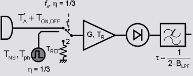
Most of (if not all) the above radiometers were conceived before the advent of the digital era. With fast analog-to-digital converters, computers and data storage systems, more sophisticated radiometer topologies have been proposed:

• The “ultra-stable radiometer” was conceived by Wilson et al. [12,13] and performs three different types of measurements: a) the noise power coming from the antenna (V_A, Equation 7), the noise power coming from the antenna plus the noise injected by the noise source (V_A+N, Equation 8), and the noise generated by the reference load (V_REF, Equation 9):

  $$V_{\mathrm{A}}=k_B\cdot \left({\mathrm{T}}_{\mathrm{A}}^{\prime }+{\mathrm{T}}_{\text{OFF}}+{\mathrm{T}}_{\mathrm{R}}\right)\cdot \mathrm{B}\cdot \mathrm{G}\cdot C_d+\text{Z}$$

  (7)

  $$V_{\mathrm{A}+\text{N}}=k_B\cdot \left({\mathrm{T}}_{\mathrm{A}}^{\prime }+{\mathrm{T}}_{\text{ON}}+{\mathrm{T}}_{\mathrm{R}}\right)\cdot \mathrm{B}\cdot \mathrm{G}\cdot C_d+\text{Z}$$

  (8)

  $$V_{\text{REF}}=k_B\cdot \left({\mathrm{T}}_{\text{REF}}{+\mathrm{T}}_{\mathrm{R}}\right)\cdot \mathrm{B}\cdot \mathrm{G}\cdot C_d+\text{Z},$$

  (9)

  where k_B is the Boltzman’s constant, and C_d and Z are the detector’s constant [V/W] and offset [V]. The three measurements (Equations 7–9) are obtained during a short period of time (τ/3 each) so that the instrument parameters can be considered as stationary (constant G and Z). They can then be combined to obtain the radiometer’s observable:

  $${\mathrm{R}}^{\text{NIR}}\widehat{=}\frac{V_{\text{REF}}-V_{\mathrm{A}}}{V_{\mathrm{A}+\text{N}}-V_{\mathrm{A}}}$$

  (10)

  from which the antenna temperature can be readily derived:

  $${\mathrm{T}}_{\mathrm{A}}^{\prime }=\left({\mathrm{T}}_{\text{REF}}-{\mathrm{T}}_{\text{OFF}}\right)-{\mathrm{R}}^{\text{NIR}}\cdot \left({\mathrm{T}}_{\text{ON}}-{\mathrm{T}}_{\text{OFF}}\right)$$

  (11)

By construction, Equation 10 is claimed to be one of the most stable data processing methods to calculate the antenna temperature [12], since R^NIR does not depend on any of the radiometer’s parameters (G, T_R, and Z). The radiometric resolution is [12,13]:

(12)

Table 1. Main types of radiometers: block diagram, basic equations and radiometric resolution.

Radiometer schematics	Radiometer basic equations	Radiometric resolution
a) Total power radiometer	$V_0=k_B\cdot \left({\mathrm{T}}_{\mathrm{A}}^{\prime }{+\mathrm{T}}_{\mathrm{R}}\right)\cdot \mathrm{B}\cdot \mathrm{G}\cdot C_d+Z$	$\mathsf{\Delta }\mathrm{T}=\left({\mathrm{T}}_{\mathrm{A}}^{\prime }{+\mathrm{T}}_{\mathrm{R}}\right)\cdot \sqrt{\frac{1}{\mathrm{B}\cdot \mathsf{\tau }}+{\left(\frac{\mathsf{\Delta }\mathrm{G}}{\mathrm{G}}\right)}^2}$
b) Dicke radiometer (unbalanced)	$V_0=\frac{1}{2}\cdot k_B\cdot \left({\mathrm{T}}_{\mathrm{A}}^{\prime }{-\mathrm{T}}_{\text{REF}}\right)\cdot \mathrm{B}\cdot \mathrm{G}\cdot C_d$	$\mathsf{\Delta }\mathrm{T}=\sqrt{\frac{2\cdot {\left({\mathrm{T}}_{\mathrm{A}}^{\prime }{+\mathrm{T}}_{\mathrm{R}}\right)}^2}{\mathrm{B}\cdot \mathsf{\tau }}+\frac{2\cdot {\left({\mathrm{T}}_{\text{REF}}{+\mathrm{T}}_{\mathrm{R}}\right)}^2}{\mathrm{B}\cdot \mathsf{\tau }}+{\left({\mathrm{T}}_{\mathrm{A}}^{\prime }{-\mathrm{T}}_{\text{REF}}\right)}^2\cdot {\left(\frac{\mathsf{\Delta }\mathrm{G}}{\mathrm{G}}\right)}^2}$
c) Balanced Dicke radiometer by duty cycle modulation	$V_0=0$   $\eta =\left({\mathrm{T}}_{\text{REF}}{+\mathrm{T}}_{\mathrm{R}}\right)/\left({\mathrm{T}}_{\mathrm{A}}^{\prime }{+\mathrm{T}}_{\text{REF}}+2\cdot {\mathrm{T}}_{\mathrm{R}}\right)$	$\mathsf{\Delta }\mathrm{T}=\sqrt{\frac{{\left({\mathrm{T}}_{\mathrm{A}}^{\prime }{+\mathrm{T}}_{\mathrm{R}}\right)}^2}{\mathrm{B}\cdot \mathsf{\tau }\cdot \eta }+\frac{{\left({\mathrm{T}}_{\text{REF}}{+\mathrm{T}}_{\mathrm{R}}\right)}^2}{\mathrm{B}\cdot \mathsf{\tau }\cdot \left(1-\eta \right)}}\hspace{0.17em}$
d) Balanced Dicke radiometer by gain modulation	$V_0=0$   $\alpha =\left({\mathrm{T}}_{\mathrm{A}}^{\prime }{+\mathrm{T}}_{\mathrm{R}}\right)/\left({\mathrm{T}}_{\text{REF}}{+\mathrm{T}}_{\mathrm{R}}\right)$	$\mathsf{\Delta }\mathrm{T}=\sqrt{\frac{2\cdot {\left({\mathrm{T}}_{\mathrm{A}}^{\prime }{+\mathrm{T}}_{\mathrm{R}}\right)}^2}{\mathrm{B}\cdot \mathsf{\tau }}+\frac{2\cdot {\left({\mathrm{T}}_{\text{REF}}{+\mathrm{T}}_{\mathrm{R}}\right)}^2}{\mathrm{B}\cdot \mathsf{\tau }}}$
e) Balanced Dicke radiometer by reference channel	$V_0=0$   ${\mathrm{T}}_{\mathrm{A}}^{\prime }{=\mathrm{T}}_{\text{REF}}^{\prime }$	$\mathsf{\Delta }\mathrm{T}=\frac{2\cdot \left({\mathrm{T}}_{\mathrm{A}}^{\prime }{+\mathrm{T}}_{\mathrm{R}}\right)}{\sqrt{\mathrm{B}\cdot \mathsf{\tau }}}$
f) Noise injection radiometer – variable noise	$V_0=0$   ${\mathrm{T}}_{\mathrm{A}}^{\prime }{+\mathrm{T}}_{\text{ON}}{=\mathrm{T}}_{\text{REF}}$	$\mathsf{\Delta }\mathrm{T}=\frac{2\cdot \left({\mathrm{T}}_{\text{REF}}{+\mathrm{T}}_{\mathrm{R}}\right)}{\sqrt{\mathrm{B}\cdot \mathsf{\tau }}}$
g) Noise injection radiometer– variable duty cycle	$V_0=0$   $\eta \cdot {\mathrm{T}}_{\text{ON}}+\left(1-\eta \right)\cdot {\mathrm{T}}_{\text{OFF}}{+\mathrm{T}}_{\mathrm{A}}{=\mathrm{T}}_{\text{REF}}$	$\mathsf{\Delta }\mathrm{T}=\frac{2\cdot \left({\mathrm{T}}_{\text{REF}}{+\mathrm{T}}_{\mathrm{R}}\right)}{\sqrt{\mathrm{B}\cdot \mathsf{\tau }}}$
h) Hach radiometer	$\begin{array}{l}{V}_0=V_{\mathrm{R}}\cdot \frac{2\cdot {\mathrm{T}}_{\mathrm{A}}^{\prime }{-\mathrm{T}}_{\text{1}}{-\mathrm{T}}_2}{{\mathrm{T}}_2{-\mathrm{T}}_{\text{1}}}\\ V_{\text{AGC}}=V_{\mathrm{R}}\\ \left(g=g_{\text{AGC}}\right)\end{array}$	$\begin{array}{l}\mathsf{\Delta }\mathrm{T}=\frac{\text{1}}{\sqrt{\mathrm{B}\cdot \mathsf{\tau }}}{\left[1+\frac{1}{1+\frac{{\tau }_{AGC}}{\tau }}{\left(\frac{{\mathrm{T}}_2{+\mathrm{T}}_{\text{1}}-2\cdot {\mathrm{T}}_{\mathrm{A}}^{\prime }}{{\mathrm{T}}_2{-\mathrm{T}}_{\text{1}}}\right)}^2\right]}^{\frac{1}{2}}\cdot \\ \hspace{1em}\hspace{1em}\cdot {\left[{\left({\mathrm{T}}_2{+\mathrm{T}}_{\mathrm{R}}\right)}^2+{\left({\mathrm{T}}_{\text{1}}{+\mathrm{T}}_{\mathrm{R}}\right)}^2+2{\left({\mathrm{T}}_{\mathrm{A}}^{\prime }{+\mathrm{T}}_{\mathrm{R}}\right)}^2\right]}^{\frac{1}{2}}\end{array}$
i) Ultra-stable radiometer	$V_{\mathrm{A}}=k_B\cdot \left({\mathrm{T}}_{\mathrm{A}}^{\prime }{+\mathrm{T}}_{\text{OFF}}{+\mathrm{T}}_{\mathrm{R}}\right)\cdot \mathrm{B}\cdot \mathrm{G}\cdot C_d+\text{Z}$ $V_{\mathrm{A}+\text{N}}=k_B\cdot \left({\mathrm{T}}_{\mathrm{A}}^{\prime }{+\mathrm{T}}_{\text{ON}}{+\mathrm{T}}_{\mathrm{R}}\right)\cdot \mathrm{B}\cdot \mathrm{G}\cdot C_d+\text{Z}$ $V_{\text{REF}}=k_B\cdot \left({\mathrm{T}}_{\text{REF}}{+\mathrm{T}}_{\mathrm{R}}\right)\cdot \mathrm{B}\cdot \mathrm{G}\cdot C_d+\text{Z}$ $R^{NIR}\widehat{=}\frac{V_{\text{REF}}-V_{\mathrm{A}}}{V_{\mathrm{A}+\text{N}}-V_{\mathrm{A}}}=\frac{{\mathrm{T}}_{\text{REF}}{-\mathrm{T}}_{\mathrm{A}}^{\prime }{-\mathrm{T}}_{\text{OFF}}}{{\mathrm{T}}_{\text{ON}}{-\mathrm{T}}_{\text{OFF}}}$	$\begin{array}{l}\mathsf{\Delta }\mathrm{T}=\sqrt{\frac{3}{\mathrm{B}·\mathsf{\tau }}}·\{{\left({\mathrm{T}}_{\text{REF}}{-\mathrm{T}}_{\text{OFF}}{+\mathrm{T}}_{\mathrm{R}}\right)}^2+{\left({\mathrm{T}}_{\mathrm{A}}^{\prime }{+\mathrm{T}}_{\mathrm{R}}\right)}^2·{\left[1-\frac{\left({\mathrm{T}}_{\text{REF}}{-\mathrm{T}}_{\text{OFF}}{-\mathrm{T}}_{\mathrm{A}}^{\prime }\right)}{{\mathrm{T}}_{\text{ON}}{-\mathrm{T}}_{\text{OFF}}}\right]}^2+\\ \hspace{1em}\hspace{1em}\hspace{1em}\hspace{1em}\hspace{1em}\hspace{1em}+{{\left({\mathrm{T}}_{\mathrm{A}}^{\prime }{+\mathrm{T}}_{\mathrm{R}}{+\mathrm{T}}_{\text{ON}}{-\mathrm{T}}_{\text{OFF}}\right)}^2·{\left[\frac{{\mathrm{T}}_{\text{REF}}{-\mathrm{T}}_{\text{OFF}}{-\mathrm{T}}_{\mathrm{A}}^{\prime }}{{\mathrm{T}}_{\text{ON}}{-\mathrm{T}}_{\text{OFF}}}\right]}^2\}}^{\frac{1}{2}}\end{array}$

Table 1. Main types of radiometers: block diagram, basic equations and radiometric resolution.

Radiometer schematics	Radiometer basic equations	Radiometric resolution
a) Total power radiometer	$V_0=k_B\cdot \left({\mathrm{T}}_{\mathrm{A}}^{\prime }{+\mathrm{T}}_{\mathrm{R}}\right)\cdot \mathrm{B}\cdot \mathrm{G}\cdot C_d+Z$	$\mathsf{\Delta }\mathrm{T}=\left({\mathrm{T}}_{\mathrm{A}}^{\prime }{+\mathrm{T}}_{\mathrm{R}}\right)\cdot \sqrt{\frac{1}{\mathrm{B}\cdot \mathsf{\tau }}+{\left(\frac{\mathsf{\Delta }\mathrm{G}}{\mathrm{G}}\right)}^2}$
b) Dicke radiometer (unbalanced)	$V_0=\frac{1}{2}\cdot k_B\cdot \left({\mathrm{T}}_{\mathrm{A}}^{\prime }{-\mathrm{T}}_{\text{REF}}\right)\cdot \mathrm{B}\cdot \mathrm{G}\cdot C_d$	$\mathsf{\Delta }\mathrm{T}=\sqrt{\frac{2\cdot {\left({\mathrm{T}}_{\mathrm{A}}^{\prime }{+\mathrm{T}}_{\mathrm{R}}\right)}^2}{\mathrm{B}\cdot \mathsf{\tau }}+\frac{2\cdot {\left({\mathrm{T}}_{\text{REF}}{+\mathrm{T}}_{\mathrm{R}}\right)}^2}{\mathrm{B}\cdot \mathsf{\tau }}+{\left({\mathrm{T}}_{\mathrm{A}}^{\prime }{-\mathrm{T}}_{\text{REF}}\right)}^2\cdot {\left(\frac{\mathsf{\Delta }\mathrm{G}}{\mathrm{G}}\right)}^2}$
c) Balanced Dicke radiometer by duty cycle modulation	$V_0=0$   $\eta =\left({\mathrm{T}}_{\text{REF}}{+\mathrm{T}}_{\mathrm{R}}\right)/\left({\mathrm{T}}_{\mathrm{A}}^{\prime }{+\mathrm{T}}_{\text{REF}}+2\cdot {\mathrm{T}}_{\mathrm{R}}\right)$	$\mathsf{\Delta }\mathrm{T}=\sqrt{\frac{{\left({\mathrm{T}}_{\mathrm{A}}^{\prime }{+\mathrm{T}}_{\mathrm{R}}\right)}^2}{\mathrm{B}\cdot \mathsf{\tau }\cdot \eta }+\frac{{\left({\mathrm{T}}_{\text{REF}}{+\mathrm{T}}_{\mathrm{R}}\right)}^2}{\mathrm{B}\cdot \mathsf{\tau }\cdot \left(1-\eta \right)}}\hspace{0.17em}$
d) Balanced Dicke radiometer by gain modulation	$V_0=0$   $\alpha =\left({\mathrm{T}}_{\mathrm{A}}^{\prime }{+\mathrm{T}}_{\mathrm{R}}\right)/\left({\mathrm{T}}_{\text{REF}}{+\mathrm{T}}_{\mathrm{R}}\right)$	$\mathsf{\Delta }\mathrm{T}=\sqrt{\frac{2\cdot {\left({\mathrm{T}}_{\mathrm{A}}^{\prime }{+\mathrm{T}}_{\mathrm{R}}\right)}^2}{\mathrm{B}\cdot \mathsf{\tau }}+\frac{2\cdot {\left({\mathrm{T}}_{\text{REF}}{+\mathrm{T}}_{\mathrm{R}}\right)}^2}{\mathrm{B}\cdot \mathsf{\tau }}}$
e) Balanced Dicke radiometer by reference channel	$V_0=0$   ${\mathrm{T}}_{\mathrm{A}}^{\prime }{=\mathrm{T}}_{\text{REF}}^{\prime }$	$\mathsf{\Delta }\mathrm{T}=\frac{2\cdot \left({\mathrm{T}}_{\mathrm{A}}^{\prime }{+\mathrm{T}}_{\mathrm{R}}\right)}{\sqrt{\mathrm{B}\cdot \mathsf{\tau }}}$
f) Noise injection radiometer – variable noise	$V_0=0$   ${\mathrm{T}}_{\mathrm{A}}^{\prime }{+\mathrm{T}}_{\text{ON}}{=\mathrm{T}}_{\text{REF}}$	$\mathsf{\Delta }\mathrm{T}=\frac{2\cdot \left({\mathrm{T}}_{\text{REF}}{+\mathrm{T}}_{\mathrm{R}}\right)}{\sqrt{\mathrm{B}\cdot \mathsf{\tau }}}$
g) Noise injection radiometer– variable duty cycle	$V_0=0$   $\eta \cdot {\mathrm{T}}_{\text{ON}}+\left(1-\eta \right)\cdot {\mathrm{T}}_{\text{OFF}}{+\mathrm{T}}_{\mathrm{A}}{=\mathrm{T}}_{\text{REF}}$	$\mathsf{\Delta }\mathrm{T}=\frac{2\cdot \left({\mathrm{T}}_{\text{REF}}{+\mathrm{T}}_{\mathrm{R}}\right)}{\sqrt{\mathrm{B}\cdot \mathsf{\tau }}}$
h) Hach radiometer	$\begin{array}{l}{V}_0=V_{\mathrm{R}}\cdot \frac{2\cdot {\mathrm{T}}_{\mathrm{A}}^{\prime }{-\mathrm{T}}_{\text{1}}{-\mathrm{T}}_2}{{\mathrm{T}}_2{-\mathrm{T}}_{\text{1}}}\\ V_{\text{AGC}}=V_{\mathrm{R}}\\ \left(g=g_{\text{AGC}}\right)\end{array}$	$\begin{array}{l}\mathsf{\Delta }\mathrm{T}=\frac{\text{1}}{\sqrt{\mathrm{B}\cdot \mathsf{\tau }}}{\left[1+\frac{1}{1+\frac{{\tau }_{AGC}}{\tau }}{\left(\frac{{\mathrm{T}}_2{+\mathrm{T}}_{\text{1}}-2\cdot {\mathrm{T}}_{\mathrm{A}}^{\prime }}{{\mathrm{T}}_2{-\mathrm{T}}_{\text{1}}}\right)}^2\right]}^{\frac{1}{2}}\cdot \\ \hspace{1em}\hspace{1em}\cdot {\left[{\left({\mathrm{T}}_2{+\mathrm{T}}_{\mathrm{R}}\right)}^2+{\left({\mathrm{T}}_{\text{1}}{+\mathrm{T}}_{\mathrm{R}}\right)}^2+2{\left({\mathrm{T}}_{\mathrm{A}}^{\prime }{+\mathrm{T}}_{\mathrm{R}}\right)}^2\right]}^{\frac{1}{2}}\end{array}$
i) Ultra-stable radiometer	$V_{\mathrm{A}}=k_B\cdot \left({\mathrm{T}}_{\mathrm{A}}^{\prime }{+\mathrm{T}}_{\text{OFF}}{+\mathrm{T}}_{\mathrm{R}}\right)\cdot \mathrm{B}\cdot \mathrm{G}\cdot C_d+\text{Z}$ $V_{\mathrm{A}+\text{N}}=k_B\cdot \left({\mathrm{T}}_{\mathrm{A}}^{\prime }{+\mathrm{T}}_{\text{ON}}{+\mathrm{T}}_{\mathrm{R}}\right)\cdot \mathrm{B}\cdot \mathrm{G}\cdot C_d+\text{Z}$ $V_{\text{REF}}=k_B\cdot \left({\mathrm{T}}_{\text{REF}}{+\mathrm{T}}_{\mathrm{R}}\right)\cdot \mathrm{B}\cdot \mathrm{G}\cdot C_d+\text{Z}$ $R^{NIR}\widehat{=}\frac{V_{\text{REF}}-V_{\mathrm{A}}}{V_{\mathrm{A}+\text{N}}-V_{\mathrm{A}}}=\frac{{\mathrm{T}}_{\text{REF}}{-\mathrm{T}}_{\mathrm{A}}^{\prime }{-\mathrm{T}}_{\text{OFF}}}{{\mathrm{T}}_{\text{ON}}{-\mathrm{T}}_{\text{OFF}}}$	$\begin{array}{l}\mathsf{\Delta }\mathrm{T}=\sqrt{\frac{3}{\mathrm{B}·\mathsf{\tau }}}·\{{\left({\mathrm{T}}_{\text{REF}}{-\mathrm{T}}_{\text{OFF}}{+\mathrm{T}}_{\mathrm{R}}\right)}^2+{\left({\mathrm{T}}_{\mathrm{A}}^{\prime }{+\mathrm{T}}_{\mathrm{R}}\right)}^2·{\left[1-\frac{\left({\mathrm{T}}_{\text{REF}}{-\mathrm{T}}_{\text{OFF}}{-\mathrm{T}}_{\mathrm{A}}^{\prime }\right)}{{\mathrm{T}}_{\text{ON}}{-\mathrm{T}}_{\text{OFF}}}\right]}^2+\\ \hspace{1em}\hspace{1em}\hspace{1em}\hspace{1em}\hspace{1em}\hspace{1em}+{{\left({\mathrm{T}}_{\mathrm{A}}^{\prime }{+\mathrm{T}}_{\mathrm{R}}{+\mathrm{T}}_{\text{ON}}{-\mathrm{T}}_{\text{OFF}}\right)}^2·{\left[\frac{{\mathrm{T}}_{\text{REF}}{-\mathrm{T}}_{\text{OFF}}{-\mathrm{T}}_{\mathrm{A}}^{\prime }}{{\mathrm{T}}_{\text{ON}}{-\mathrm{T}}_{\text{OFF}}}\right]}^2\}}^{\frac{1}{2}}\end{array}$

2. Radiometric Resolution Optimization Using Variable Integration Times

At this point, it is worth to ask ourselves if the radiometric resolution of the above radiometers can be improved, while—at the same time—having a radiometer topology that is insensitive to gain, receiver’s noise temperature, and detector offsets fluctuations. From the above strategies to mitigate gain and, eventually, receiver’s noise temperature, the only ones that provide some tuning capabilities are the Dicke radiometer, with duty-cycle modulation, and the “ultra-stable radiometer”, for which different measurement times for each observable can be adjusted. It is important to note that the observations of the Dicke reference load and the additive noise from an injected noise source (V_REF and V_A+N; Equations 8 and 9 of the ultra-stable radiometer) are intrinsically part of the measurement strategy to obtain the radiometer’s raw observables to yield to a significant reduction in the fluctuations of the radiometer output. The observation times associated to these references must then be included in the total observation time (=radiometer’s integration time) [14,15], which is given by:

$$\mathsf{\tau }={\mathsf{\tau }}_{\text{REF}}+{\mathsf{\tau }}_{\mathrm{A}}+{\mathsf{\tau }}_{\mathrm{A}+\text{N}}.$$

(13)

The ultimate absolute calibration is then performed using, for example, the hot load-cold load technique [14,15] or tip-curves [17]. The observation times of these targets must not be included in the integration time, since these are different measurements themselves.

The derivation of the radiometric resolution of the Dicke radiometer with duty-cycle modulation is straight-forward (Equation 3) and the integration times are determined by the balancing equation.

The radiometric resolution of the ultra-stable NIR configuration can be calculated following the methodology described by [13]. It is convenient to consider each of the output measurements to be equal to its expected value plus a random term, if the relative error in each measurement is small (Equations 7–9) and conditions are stationary. The random term is a small fraction of the expected value and can be modeled as an additive zero-mean random Gaussian variable: ${\text{P}}_i=\overline{{\text{P}}_i}\left(1+{\mathsf{\delta }}_i\right)$ where δ_i represents the random term of the i measurement (Equations 7–9), with variance $\overline{{\mathsf{\delta }}_{\text{i}}^2}=1/\left(B\cdot {\mathsf{\tau }}_i\right)$, where τ_i represent the measurement time.

Substituting these equations in Equation 10:

$${\mathrm{R}}^{\text{NIR}}=\frac{\overline{V_{\text{REF}}}\left(1+{\mathsf{\delta }}_{\text{REF}}\right)-\overline{V_{\mathrm{A}}}\left(1+{\mathsf{\delta }}_{\mathrm{A}}\right)}{\overline{V_{\mathrm{A}+\text{N}}}\left(1+{\mathsf{\delta }}_{\mathrm{A}+\text{N}}\right)-\overline{V_{\mathrm{A}}}\left(1+{\mathsf{\delta }}_{\mathrm{A}}\right)}=\frac{\left(\overline{V_{\text{REF}}}-\overline{V_{\mathrm{A}}}\right)+\overline{V_{\text{REF}}}\hspace{0.17em}{\mathsf{\delta }}_{\text{REF}}-\overline{V_{\mathrm{A}}}\hspace{0.17em}{\mathsf{\delta }}_{\mathrm{A}}}{1+\frac{\overline{V_{\mathrm{A}+\text{N}}}}{\overline{V_{\mathrm{A}+\text{N}}}-\overline{V_{\mathrm{A}}}}{\mathsf{\delta }}_{\mathrm{A}+\text{N}}-\frac{\overline{V_{\mathrm{A}}}}{\overline{V_{\mathrm{A}+\text{N}}}-\overline{V_{\mathrm{A}}}}{\mathsf{\delta }}_{\mathrm{A}}}\frac{1}{\overline{V_{\mathrm{A}+\text{N}}}-\overline{V_{\mathrm{A}}}}$$

(14)

The random terms are assumed to be much smaller than 1. Therefore, retaining the first order terms only, Equation 14 can be simplified as:

$${\mathrm{R}}^{\text{NIR}}\widehat{=}\frac{\left(\overline{V_{\text{REF}}}-\overline{V_{\mathrm{A}}}\right)+\overline{V_{\text{REF}}}\cdot {\mathsf{\delta }}_{\text{REF}}-\left(1-\overline{{\mathrm{R}}^{\text{NIR}}}\right)\cdot \overline{V_{\mathrm{A}}}\cdot {\mathsf{\delta }}_{\mathrm{A}}-\overline{{\mathrm{R}}^{\text{NIR}}}\cdot \overline{V_{\mathrm{A}+\text{N}}}\cdot {\mathsf{\delta }}_{\mathrm{A}+\text{N}}}{\overline{V_{\mathrm{A}+\text{N}}}-\overline{V_{\mathrm{A}}}}$$

(15)

where:

$$\overline{{\mathrm{R}}^{\text{NIR}}}\widehat{=}\frac{\overline{V_{\text{REF}}}-\overline{V_{\mathrm{A}}}}{\overline{V_{\mathrm{A}+\text{N}}}-\overline{V_{\mathrm{A}}}}=\frac{{\mathrm{T}}_{\text{REF}}{-\mathrm{T}}_{\mathrm{A}}^{\prime }{-\mathrm{T}}_{\text{OFF}}}{{\mathrm{T}}_{\text{ON}}{-\mathrm{T}}_{\text{OFF}}}$$

(16)

Substituting Equations 7–9 in Equation 15, the antenna temperature can be computed as:

$${\widehat{\mathrm{T}}}_{\mathrm{A}}{\widehat{=}\mathrm{T}}_{\mathrm{A}}\text{+}{\epsilon }_{{\mathrm{T}}_{\mathrm{A}}}{=\mathrm{T}}_{\mathrm{A}}-\left({\mathrm{T}}_{\text{REF}}{+\mathrm{T}}_{\mathrm{R}}\right)\cdot {\mathsf{\delta }}_{\text{REF}}-\left(1-\overline{{\mathrm{R}}^{\text{NIR}}}\right)\left({\mathrm{T}}_{\mathrm{A}}^{\prime }{+\mathrm{T}}_{\text{OFF}}{+\mathrm{T}}_{\mathrm{R}}\right)\cdot {\mathsf{\delta }}_{\mathrm{A}}-\overline{{\mathrm{R}}^{\text{NIR}}}\cdot \left({\mathrm{T}}_{\mathrm{A}}^{\prime }{+\mathrm{T}}_{\text{ON}}{+\mathrm{T}}_{\mathrm{R}}\right)\cdot {\mathsf{\delta }}_{\mathrm{A}+\text{N}}$$

(17)

${\mathsf{\epsilon }}_{{\mathrm{T}}_{\mathrm{A}}}$ in Equation 17 represents the error introduced in the radiometric measurements. The radiometric resolution can then be computed as the quadratic sum of the components of this error term:

$$\begin{array}{l}\mathsf{\Delta }\mathrm{T}=\sqrt{\frac{{\left({\mathrm{T}}_{\text{REF}}{+\mathrm{T}}_{\mathrm{R}}\right)}^2}{\mathrm{B}\cdot {\mathsf{\tau }}_{\text{REF}}}+\frac{{\left(1-\overline{{\mathrm{R}}^{\text{NIR}}}\right)}^2\cdot {\left({\mathrm{T}}_{\mathrm{A}}^{\prime }{+\mathrm{T}}_{\text{OFF}}{+\mathrm{T}}_{\mathrm{R}}\right)}^2}{\mathrm{B}\cdot {\mathsf{\tau }}_{\mathrm{A}}}+\frac{{\overline{{\mathrm{R}}^{\text{NIR}}}}^2\cdot {\left({\mathrm{T}}_{\mathrm{A}}^{\prime }{+\mathrm{T}}_{\text{ON}}{+\mathrm{T}}_{\mathrm{R}}\right)}^2}{\mathrm{B}\cdot {\mathsf{\tau }}_{\mathrm{A}+\text{N}}}}=\\ \hspace{1em}\hspace{0.17em}\hspace{0.17em}=\sqrt{\frac{{\left({\mathrm{T}}_{\text{REF}}{+\mathrm{T}}_{\mathrm{R}}\right)}^2}{\mathrm{B}\cdot {\mathsf{\tau }}_{\text{REF}}}+\frac{1}{\mathrm{B}\cdot {\mathsf{\tau }}_{\mathrm{A}}}\cdot \frac{{\left({\mathrm{T}}_{\text{ON}}{-\mathrm{T}}_{\text{REF}}{+\mathrm{T}}_{\mathrm{A}}\right)}^2\cdot {\left({\mathrm{T}}_{\mathrm{A}}^{\prime }{+\mathrm{T}}_{\text{OFF}}{+\mathrm{T}}_{\mathrm{R}}\right)}^2}{{\left({\mathrm{T}}_{\text{ON}}{-\mathrm{T}}_{\text{OFF}}\right)}^2}+\frac{\text{1}}{\mathrm{B}\cdot {\mathsf{\tau }}_{\mathrm{A}+\text{N}}}\frac{{\left({\mathrm{T}}_{\text{REF}}{-\mathrm{T}}_{\text{OFF}}{-\mathrm{T}}_{\mathrm{A}}^{\prime }\right)}^2\cdot {\left({\mathrm{T}}_{\mathrm{A}}^{\prime }{+\mathrm{T}}_{\text{ON}}{+\mathrm{T}}_{\mathrm{R}}\right)}^2}{{\left({\mathrm{T}}_{\text{ON}}{-\mathrm{T}}_{\text{OFF}}\right)}^2}}.\end{array}$$

(18)

To obtain the minimum radiometric resolution the optimum measurement times must be found assuming that τ = τ_A + τ_A+N + τ_REF is a constant. Therefore, one of the three measurement times can be expressed as a function of the other two, for example: τ_A = τ − τ_A+N − τ_REF. The optimum measurement times are then obtained by solving the following equations:

$$\frac{\partial \left(\mathsf{\Delta }{\mathrm{T}}^2\right)}{\partial {\tau }_{\text{REF}}}=0,\frac{\partial \left(\mathsf{\Delta }{\mathrm{T}}^2\right)}{\partial {\tau }_{\mathrm{A}+\text{N}}}=0.$$

(19)

Replacing Equation 18 in Equation 19 the following system of equations are obtained:

$$\frac{{\left(\mathsf{\tau }-{\mathsf{\tau }}_{\text{REF}}-{\mathsf{\tau }}_{\mathrm{A}+\text{N}}\right)}^2}{{\mathsf{\tau }}_{\mathrm{A}+\text{N}}^2}={\left(\frac{\left({\mathrm{T}}_{\mathrm{A}}+{\mathrm{T}}_{\text{OFF}}+{\mathrm{T}}_{\mathrm{R}}\right)\cdot \left({\mathrm{T}}_{\mathrm{A}}+{\mathrm{T}}_{\text{ON}}-{\mathrm{T}}_{\text{REF}}\right)}{\left({\mathrm{T}}_{\mathrm{A}}+{\mathrm{T}}_{\text{ON}}+{\mathrm{T}}_{\mathrm{R}}\right)\cdot \left({\mathrm{T}}_{\text{REF}}-{\mathrm{T}}_{\text{OFF}}-{\mathrm{T}}_{\mathrm{A}}\right)}\right)}^2$$

(20)

and

$$\frac{{\left(\mathsf{\tau }-{\mathsf{\tau }}_{\text{REF}}-{\mathsf{\tau }}_{\mathrm{A}+\text{N}}\right)}^2}{{\mathsf{\tau }}_{\mathrm{A}+\text{N}}^2}={\left(\frac{\left({\mathrm{T}}_{\mathrm{A}}+{\mathrm{T}}_{\text{OFF}}+{\mathrm{T}}_{\mathrm{R}}\right)\cdot \left({\mathrm{T}}_{\mathrm{A}}+{\mathrm{T}}_{\text{ON}}-{\mathrm{T}}_{\text{REF}}\right)}{\left({\mathrm{T}}_{\mathrm{A}}+{\mathrm{T}}_{\text{ON}}+{\mathrm{T}}_{\mathrm{R}}\right)\cdot \left({\mathrm{T}}_{\text{REF}}-{\mathrm{T}}_{\text{OFF}}-{\mathrm{T}}_{\mathrm{A}}\right)}\right)}^2$$

(21)

from which τ_A+N and τ_REF are derived:

$$\mathsf{\tau }-{\mathsf{\tau }}_{\mathrm{A}+\text{N}}={\mathsf{\tau }}_{\text{REF}}\left(1\pm \frac{\left({\mathrm{T}}_{\mathrm{A}}+{\mathrm{T}}_{\text{OFF}}+{\mathrm{T}}_{\mathrm{R}}\right)\cdot \left({\mathrm{T}}_{\mathrm{A}}+{\mathrm{T}}_{\text{ON}}-{\mathrm{T}}_{\text{REF}}\right)}{\left({\mathrm{T}}_{\text{REF}}+{\mathrm{T}}_{\mathrm{R}}\right)\cdot \left({\mathrm{T}}_{\text{ON}}-{\mathrm{T}}_{\text{REF}}\right)}\right)$$

(22)

$$\mathsf{\tau }-{\mathsf{\tau }}_{\text{REF}}={\mathsf{\tau }}_{\mathrm{A}+\text{N}}\left(1\pm \frac{\left({\mathrm{T}}_{\mathrm{A}}+{\mathrm{T}}_{\text{OFF}}+{\mathrm{T}}_{\mathrm{R}}\right)\cdot \left({\mathrm{T}}_{\text{ON}}+{\mathrm{T}}_{\mathrm{A}}-{\mathrm{T}}_{\text{REF}}\right)}{\left({\mathrm{T}}_{\mathrm{A}}+{\mathrm{T}}_{\text{ON}}+{\mathrm{T}}_{\mathrm{R}}\right)\cdot \left({\mathrm{T}}_{\text{REF}}-{\mathrm{T}}_{\text{OFF}}-{\mathrm{T}}_{\mathrm{A}}\right)}\right).$$

(23)

From Equations 22 and 23, four solutions can be obtained (+ +, + –, – + and – – within the parentheses). After a mathematical analysis of the four possible combinations of solutions, only two are possible:

(1) the solution obtained from Equations 22 and 23 corresponding to case (+ +) is valid for ${\mathrm{T}}_{\mathrm{A}}\le {\mathrm{T}}_{\text{REF}}{-\mathrm{T}}_{\text{OFF}}$ with the following optimum integration times:

$$\{\begin{array}{l}{\mathsf{\tau }}_{\text{REF}}=\frac{\mathsf{\tau }}{2},\\ {\mathsf{\tau }}_{\mathrm{A}+\text{N}}=\frac{\mathsf{\tau }}{2}\cdot \frac{\left({\mathrm{T}}_{\mathrm{A}}+{\mathrm{T}}_{\text{OFF}}+{\mathrm{T}}_{\mathrm{R}}\right)\cdot \left({\mathrm{T}}_{\text{REF}}-{\mathrm{T}}_{\text{OFF}}-{\mathrm{T}}_{\mathrm{A}}\right)}{\left({\mathrm{T}}_{\text{REF}}+{\mathrm{T}}_{\mathrm{R}}\right)\cdot \left({\mathrm{T}}_{\text{ON}}-{\mathrm{T}}_{\text{OFF}}\right)},\\ {\mathsf{\tau }}_{\mathrm{A}}=\mathsf{\tau }-{\mathsf{\tau }}_{\mathrm{A}+\text{N}}-{\mathsf{\tau }}_{\text{REF}}.\end{array}.$$

(24)

and

(2) the solution composed by Equations 22 and 23 corresponding to case (+ –) is valid for ${\mathrm{T}}_{\mathrm{A}}\ge {\mathrm{T}}_{\text{REF}}{-\mathrm{T}}_{\text{OFF}}$ with the following optimum integration times:

$$\{\begin{array}{l}{\mathsf{\tau }}_{\text{REF}}=\frac{\mathsf{\tau }}{2}\cdot \frac{\left({\mathrm{T}}_{\text{REF}}+{\mathrm{T}}_{\mathrm{R}}\right)\cdot \left({\mathrm{T}}_{\text{ON}}-{\mathrm{T}}_{\text{OFF}}\right)}{\left({\mathrm{T}}_{\mathrm{A}}+{\mathrm{T}}_{\text{OFF}}+{\mathrm{T}}_{\mathrm{R}}\right)\cdot \left({\mathrm{T}}_{\mathrm{A}}+{\mathrm{T}}_{\text{ON}}-{\mathrm{T}}_{\text{REF}}\right)},\\ {\mathsf{\tau }}_{\mathrm{A}+\text{N}}=\frac{\mathsf{\tau }}{2}\cdot \frac{\left({\mathrm{T}}_{\mathrm{A}}+{\mathrm{T}}_{\text{ON}}+{\mathrm{T}}_{\mathrm{R}}\right)\cdot \left({\mathrm{T}}_{\mathrm{A}}-{\mathrm{T}}_{\text{REF}}+{\mathrm{T}}_{\text{OFF}}\right)}{\left({\mathrm{T}}_{\mathrm{A}}+{\mathrm{T}}_{\text{OFF}}+{\mathrm{T}}_{\mathrm{R}}\right)\cdot \left({\mathrm{T}}_{\mathrm{A}}+{\mathrm{T}}_{\text{ON}}-{\mathrm{T}}_{\text{REF}}\right)},\\ {\mathsf{\tau }}_{\mathrm{A}}=\mathsf{\tau }-{\mathsf{\tau }}_{\mathrm{A}+\text{N}}-{\mathsf{\tau }}_{\text{REF}}=\frac{\mathsf{\tau }}{2}.\end{array}$$

(25)

Equations 24 and 25 depend only on T_A as all the other radiometer parameters are constant. Replacing Equations 24 or 25 in 18, the optimum radiometric resolution is readily obtained.

3. Numerical Results

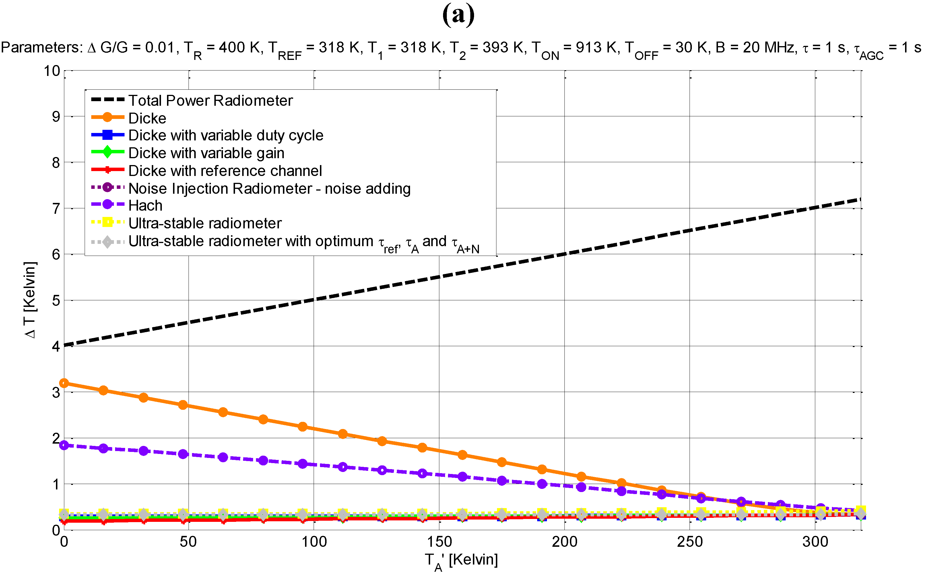
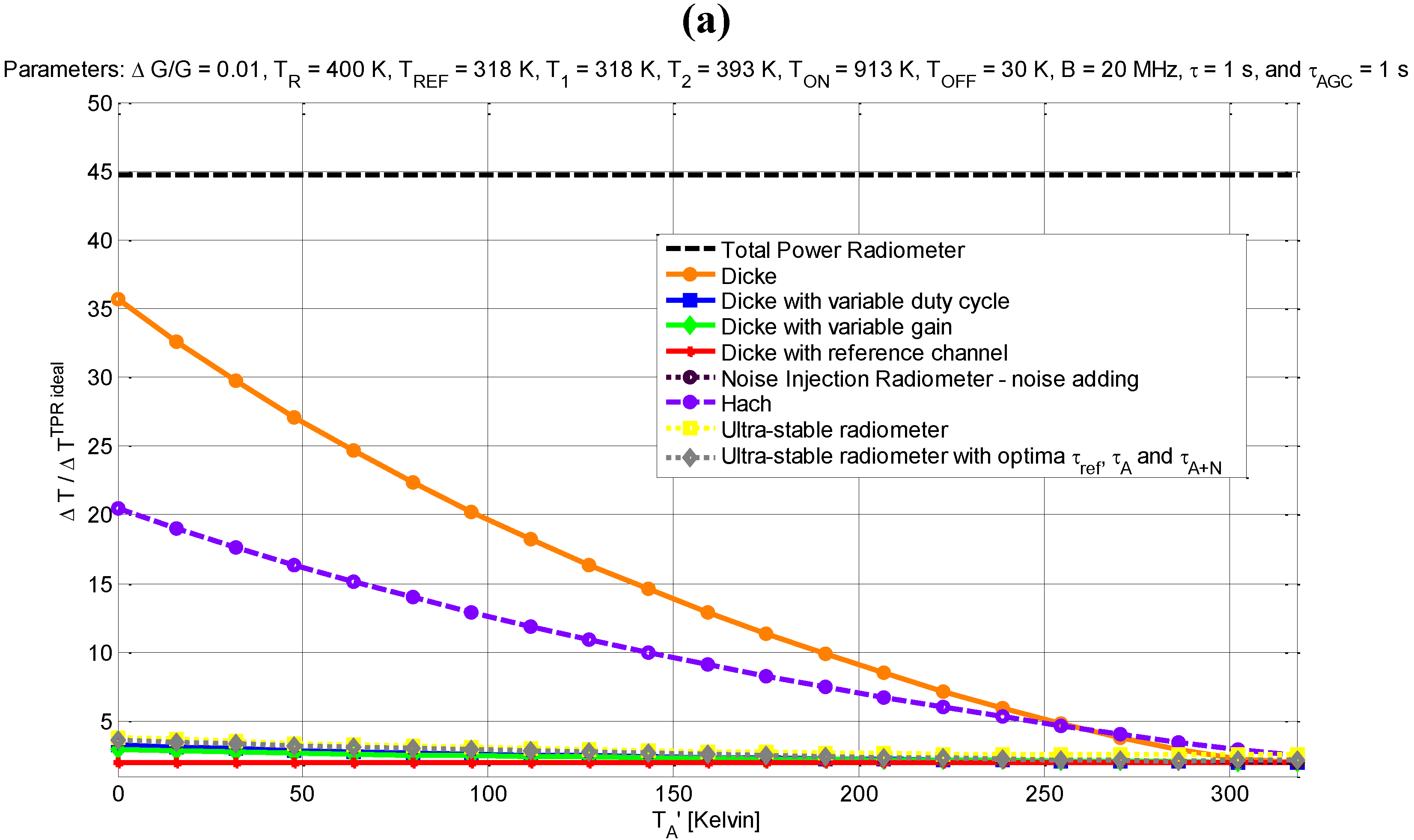
Figure 1, Figure 2, Figure 3 and Figure 4 show the numerical results as a function of the antenna temperature, evaluating the above expressions with the following parameters: $\mathsf{\Delta }\mathrm{G}/\mathrm{G}=0.01$, T_R = 1,000 K, T_REF = 318 K (45 °C), T₁ = 318 K, T₂ = 393 K, T_ON = 913 K, T_OFF = 30 K, B = 20 MHz, τ = 1 s, and τ_AGC = 1 s. 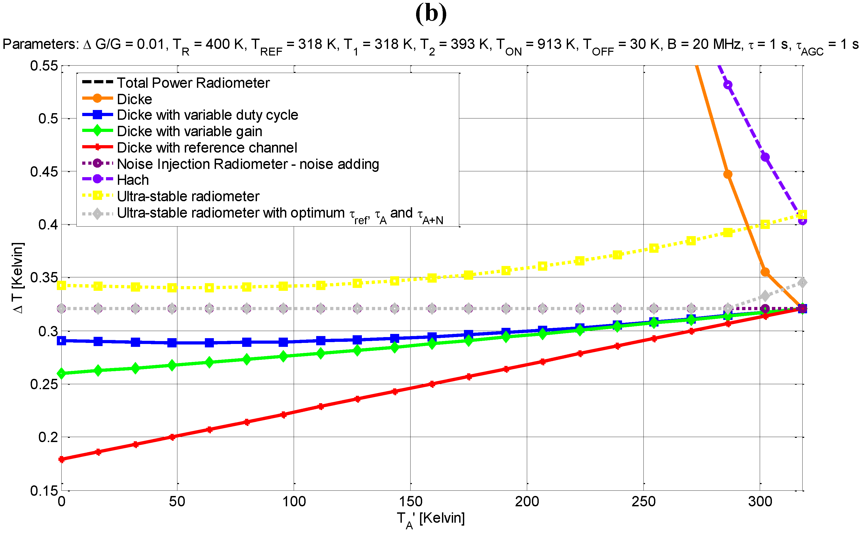As it can be appreciated, in Figure 1a, the radiometric resolution of the total power radiometer increases with increasing T_A, while decreases for the Dicke and Hach radiometers as they get balanced, and it is very similar and fairly constant (or exhibits a small increase) for the other radiometer types, which are balanced (Figure 1b).

Figure 1. (a) Radiometric resolution of different types of microwave radiometers with ΔG/G = 0.01, T_R = 400 K, T_REF = 318 K, T₁ = 318 K, T₂ = 393 K, T_ON = 913 K, T_OFF = 30 K, B = 20 MHz, τ = 1 s, τ_AGC = 1 s, (b) Zoom of Figure 1(a).

Figure 1. (a) Radiometric resolution of different types of microwave radiometers with ΔG/G = 0.01, T_R = 400 K, T_REF = 318 K, T₁ = 318 K, T₂ = 393 K, T_ON = 913 K, T_OFF = 30 K, B = 20 MHz, τ = 1 s, τ_AGC = 1 s, (b) Zoom of Figure 1(a).

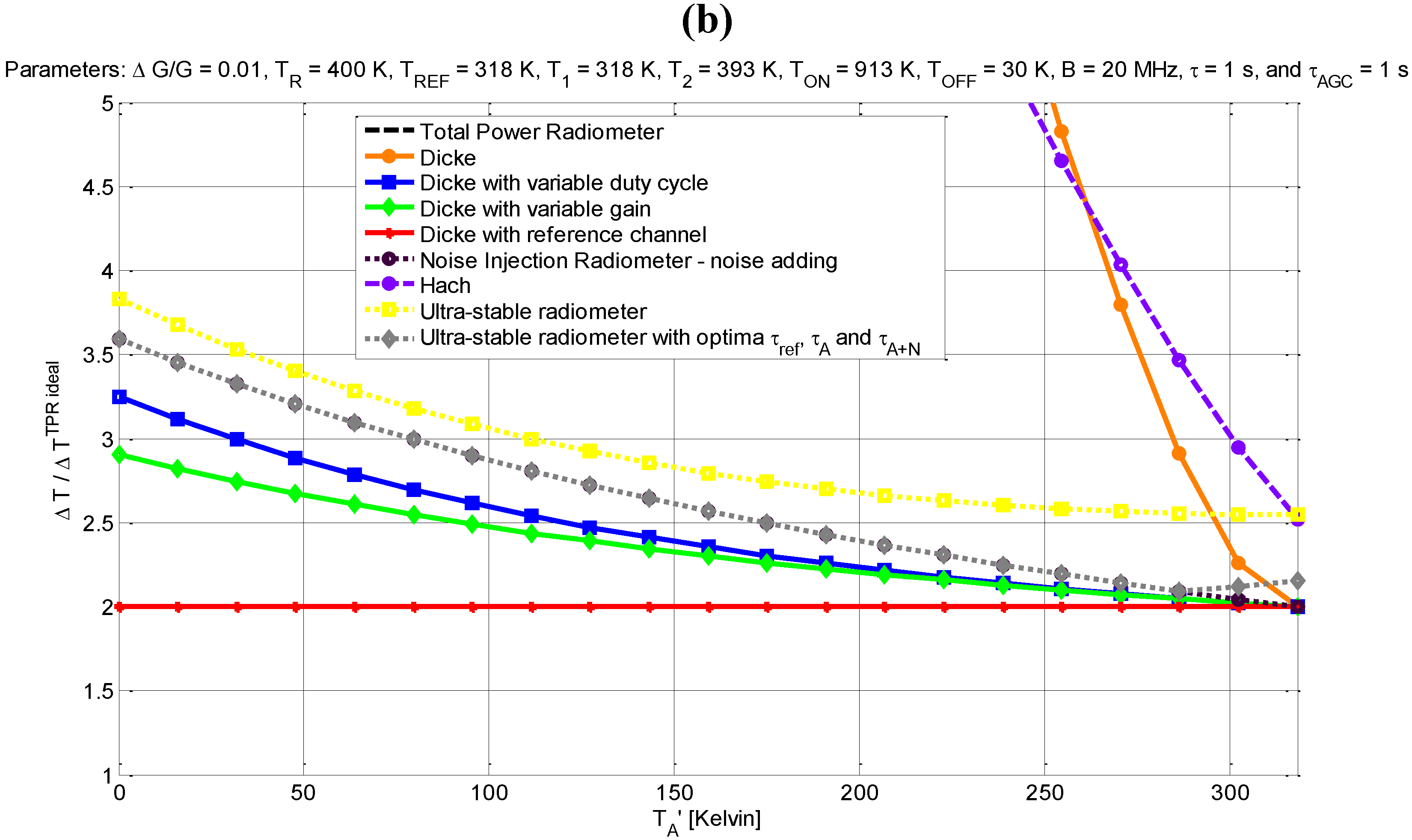
Figure 2a shows the relative performance of the radiometric resolution as compared to that of an ideal total power radiometer. As expected, the worst performance is given by the total power radiometer, which does not compensate the gain fluctuations by any means. This relative performance is constant for all T_A values. In terms of relative performance, the Dicke and Hach radiometers follow, improving with increasing T_A, as they get balanced. For all other radiometer types, their relative performance is very similar and improves with T_A approaching T_REF as the radiometers need less extra noise or can afford larger observation times of the antenna signal (Figure 2b).

Figure 2. (a) Radiometric resolution of different types of microwave radiometers normalized to the one of an ideal total power radiometer ((1) with ΔG/G = 0) with ΔG/G = 0.01, T_R = 400 K, T_REF = 318 K, T₁ = 318 K, T₂ = 393 K, T_ON = 913 K, T_OFF = 30 K, B = 20 MHz, τ = 1 s, τ_AGC = 1 s, (b) Zoom of Figure 2(a).

Figure 2. (a) Radiometric resolution of different types of microwave radiometers normalized to the one of an ideal total power radiometer ((1) with ΔG/G = 0) with ΔG/G = 0.01, T_R = 400 K, T_REF = 318 K, T₁ = 318 K, T₂ = 393 K, T_ON = 913 K, T_OFF = 30 K, B = 20 MHz, τ = 1 s, τ_AGC = 1 s, (b) Zoom of Figure 2(a).

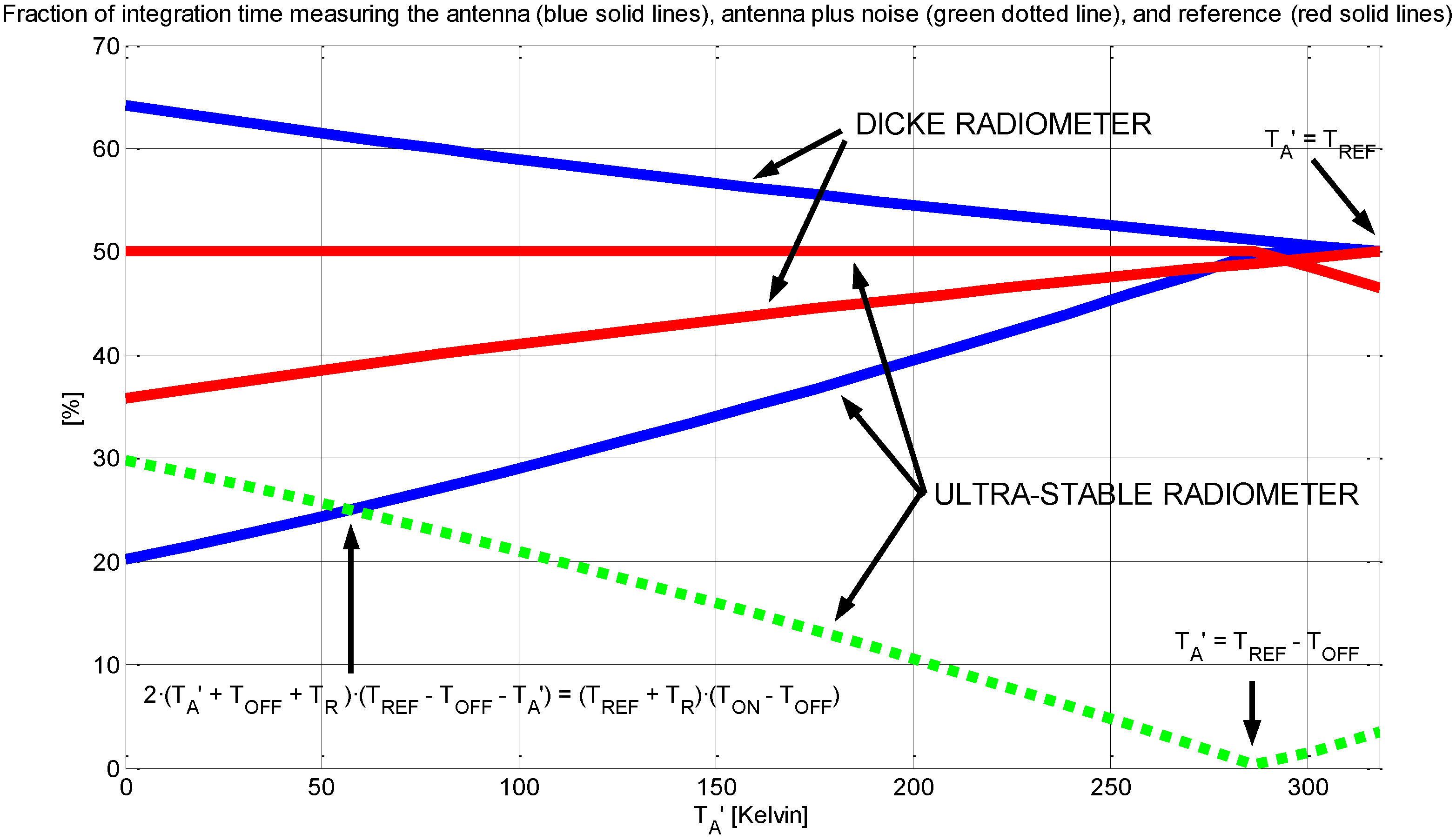
Figure 3 shows the evolution of the relative observation times spent in the antenna (solid blue line), antenna + noise (dotted green line) or reference (solid red line) for the ultra-stable and Dicke radiometers with duty-cycle modulation. For the ultra-stable radiometer, a slope change occurs at T_A = T_REF − T_OFF. Note that the crossing point depends on T_R for the ultra-stable radiometer (among several other parameters). For the Dicke radiometer with duty-cycle modulations the cross-point occurs at T_A = T_REF, below that point, larger observation times are required to the antenna signal, since it is weaker than the reference temperature.

Figure 3. Fractions of integration time spent in the antenna (solid blue lines), antenna + noise (dotted green line) or reference (solid red lines) for the ultra-stable and Dicke radiometers with duty-cycle modulation. For the ultra-stable radiometer a slope change occurs at T_A = T_REF - T_OFF. Note that the cross point depends on T_R for the ultra-stable radiometer (among several other parameters). For the Dicke radiometer with duty-cycle modulations the cross-point occurs at T_A = T_REF.

Figure 3. Fractions of integration time spent in the antenna (solid blue lines), antenna + noise (dotted green line) or reference (solid red lines) for the ultra-stable and Dicke radiometers with duty-cycle modulation. For the ultra-stable radiometer a slope change occurs at T_A = T_REF - T_OFF. Note that the cross point depends on T_R for the ultra-stable radiometer (among several other parameters). For the Dicke radiometer with duty-cycle modulations the cross-point occurs at T_A = T_REF.

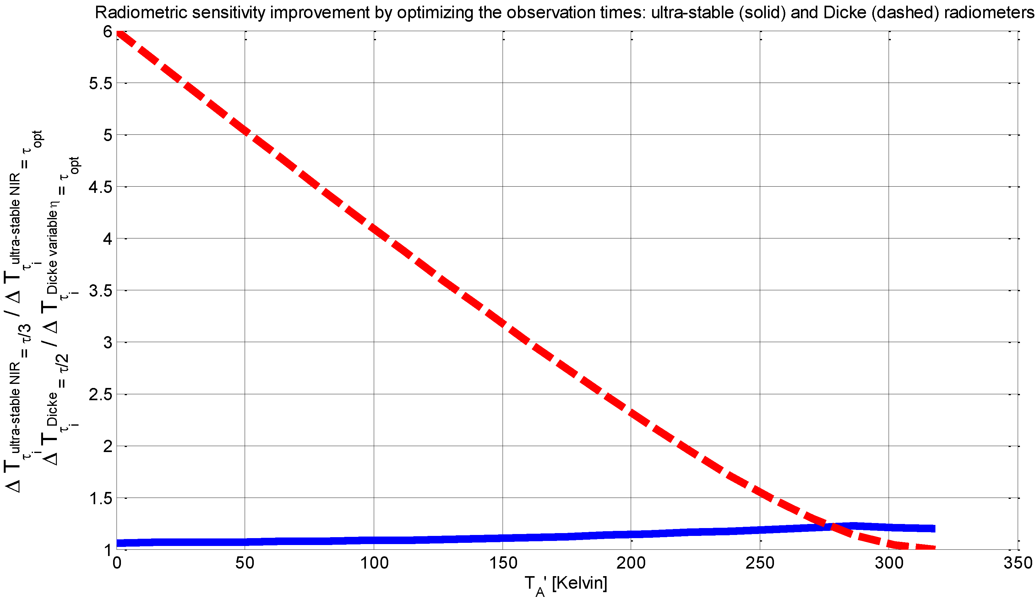
Finally, Figure 4 shows the radiometric resolution improvement for the ultra-stable radiometer (solid line) and the Dicke radiometer with duty-cycle modulation (dashed line). For the ultra-stable radiometer the improvement is moderate, about 6–22%, but not negligible, especially at high antenna temperatures. For the Dicke radiometer the improvement is very significant, especially at low antenna temperatures, when the radiometer is less balanced.

Figure 4. Radiometric resolution improvement for the ultra-stable radiometer. For the ultra-stable radiometer the improvement is about 6–22%, (while for the Dicke radiometer can be a factor of ~11).

Figure 4. Radiometric resolution improvement for the ultra-stable radiometer. For the ultra-stable radiometer the improvement is about 6–22%, (while for the Dicke radiometer can be a factor of ~11).

4. Experimental Results

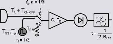
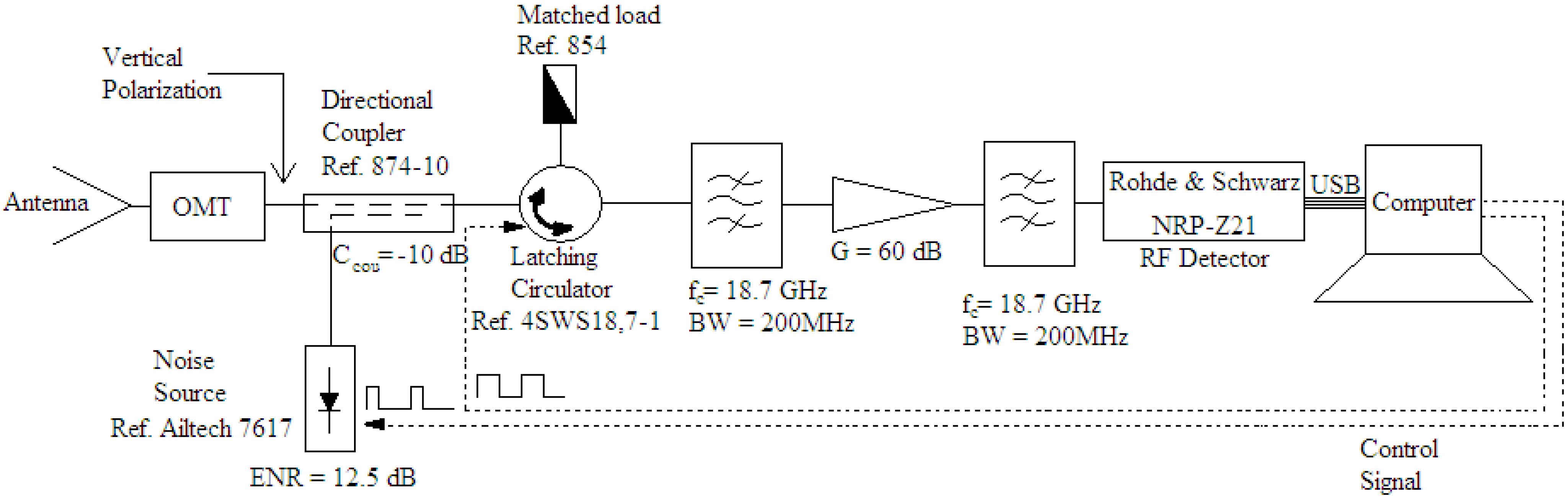
In this section, the radiometric resolution and stability performance of a K-band radiometer designed and implemented for academic purposes are presented. Its performance has not been optimized in terms of stability or radiometric resolution, but rather, it tries to show the different performances in different operation modes. The radiometer’s topology is shown in Figure 5 and it can be operated as a NIR (noise pulses are injected and latching circulator switches between the antenna and the matched load), a Dicke (noise source is OFF, but latching circulator switches between the antenna and the matched load), or a TPR (noise source is OFF and latching circulator connects the antenna to the receiver’s input). In this way, a fair comparison between different radiometer types with exactly the same hardware is performed. The main hardware parameters are: coupling = 10 dB (C = 0.1), receiver’s noise temperature T_R = 957 K, equivalent noise source temperature T_NS = 5,959 K, and T_ph = 318 K. Radiometer’s calibration is performed using the hot-cold load technique [14,15], using a microwave absorber at a known physical temperature as hot load, and a zenith view of the sky in a clear day as the cold load.

Figure 5. A block diagram of the K-band radiometer.

Figure 5. A block diagram of the K-band radiometer.

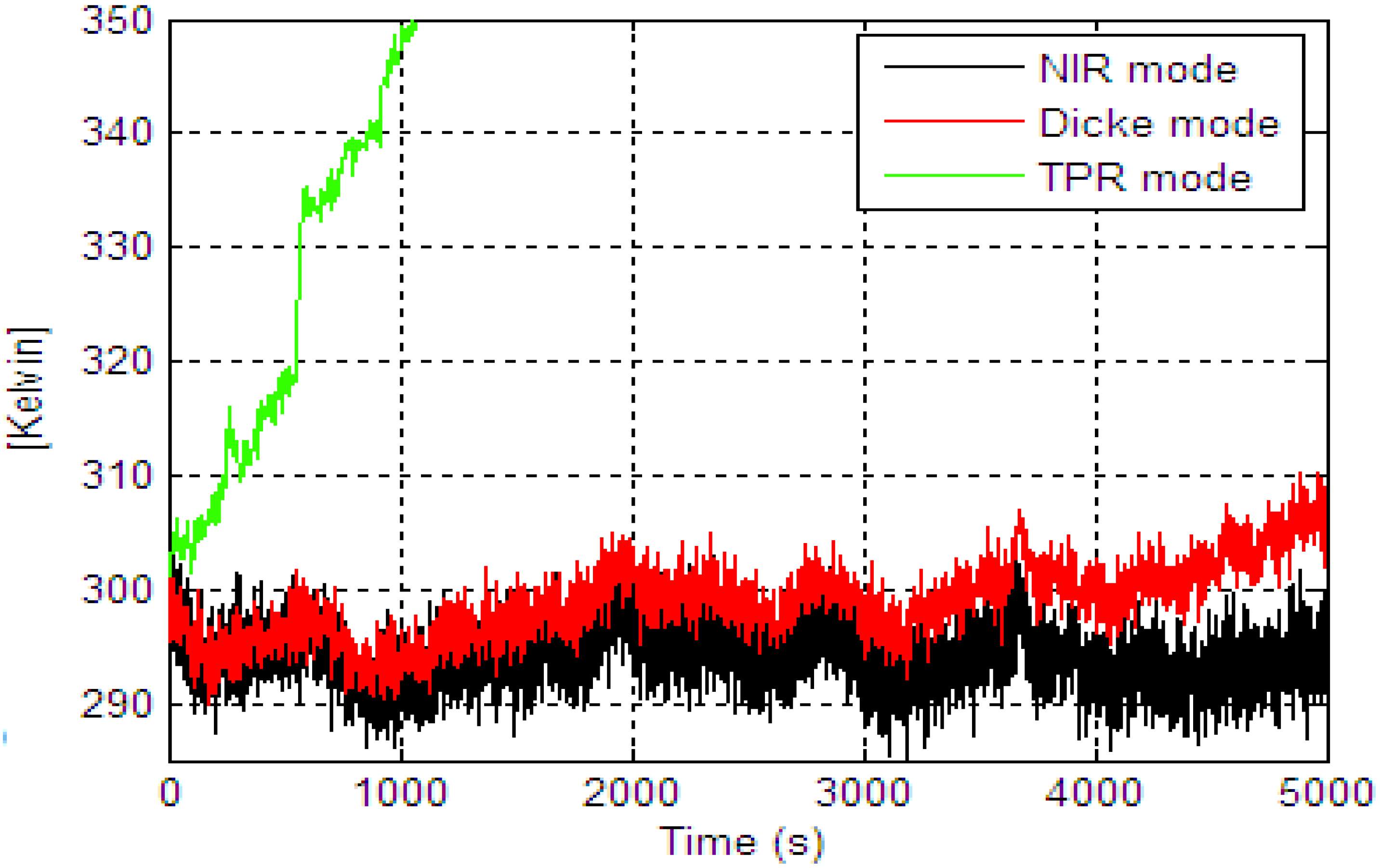
To show the measurement’s uncertainty (including radiometric resolution, non-stationary fluctuations, and calibration errors) at τ = 1 s, an outdoor measurement of 5,000 samples of 1 s of total integration time (10-times the basic integration time τ^NIR = 100 ms) pointing to a microwave absorber was performed.

As can be seen in Figure 6, the stability of the three modes is very different. For the case of the NIR mode, there is a ~4 K/°C thermal drift produced by variations in the physical temperature inside the radiometer box. These variations can only be minimized with a better temperature control and a software compensation knowing the physical temperature at different points of the radiometer box. As expected for the Dicke mode, the drifts are more pronounced than in the NIR case due to the RF amplifiers gain fluctuations, and are about 10 K in 5,000 s. For the TPR case, the drifts are huge, about 50 K in 1,000 s, and frequent absolute calibration is mandatory every few seconds at most.

Figure 6. The measured antenna temperature for the three modes of operation of the K-band radiometer.

Figure 6. The measured antenna temperature for the three modes of operation of the K-band radiometer.

To estimate the radiometric resolution term only, thermal drifts are removed first from the measured antenna temperatures by using a linear de-trend, and finally the rms values are computed. The estimated radiometric sensitivity values for the three modes of operation are: ΔT^NIR = 1.76 K; ΔT^Dicke = 1.21 K; and ΔT^TPR = 0.65 K. The relationships between the sensitivities obtained from the three different modes of operation are very close to the theoretical relationship: ΔT^Dicke/ΔT^TPR = 1.85 and ΔT^NIR/ΔT^TPR = 2.69, quite close to the theoretical values (2 and 2.62) [15].

A measurement of the stability is obtained from the Allan variance (σ_y²) [18], and provides the longest integration time (τ) for which the best radiometric sensitivity can be obtained:

$${{\mathsf{\sigma }}_{\text{y}}}^2\left(\mathsf{\tau }\right)=\frac{1}{2\left(\text{N}-1\right)}{\displaystyle \sum _{i=1}^{\text{N}-1}{\left({\text{y}}_{i+1}-{\text{y}}_i\right)}^2},$$

(26)

where: N is the number of measurements in τ seconds, and y_i is the i^th measurement.

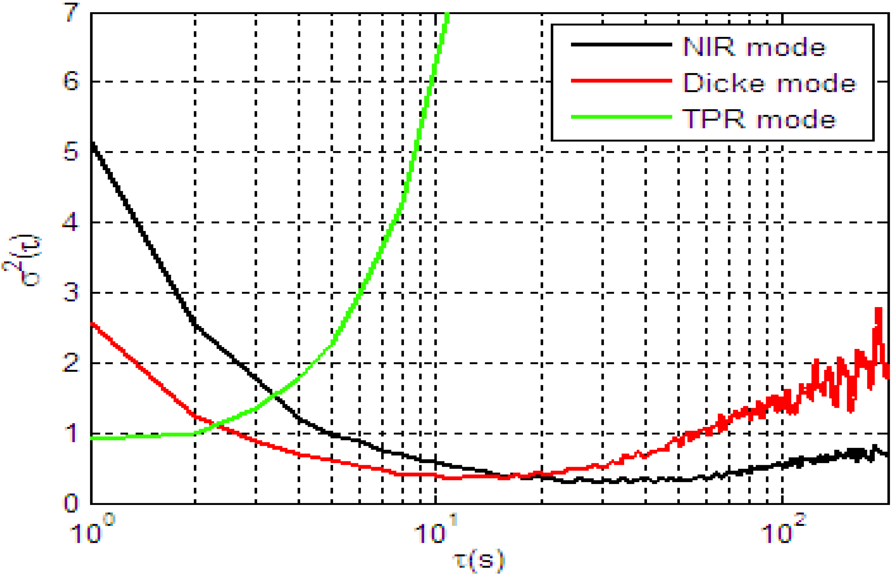
Results are shown in Figure 7, and as it can be observed the TPR mode has the lowest Allan variance value for the shortest integration times (σ² = 0.92 K² at τ = 1s → $\mathsf{\Delta }{\mathrm{T}}_{\text{min}}^{\text{TPR}}=0.96\hspace{0.17em}\text{K}$), followed by the DR mode, for medium integration times (σ² = 0.34 K² at τ = 11s → $\mathsf{\Delta }{\mathrm{T}}_{\text{min}}^{\text{Dicke}}=0.58\hspace{0.17em}\text{K}$), and finally, the NIR mode, which has the lowest Allan’s variance value (highest stability) for longest integration times (σ² = 0.28 K² at τ = 42s → $\mathsf{\Delta }{\mathrm{T}}_{\text{min}}^{\text{NIR}}=0.53\hspace{0.17em}\text{K}$). Note that these integration times have been optimized on a snapshot basis only, and could be improved even further by reference averaging to the whole system [12,19], and for the case of the Dicke mode, gain averaging as well [12].

Figure 7. Allan variance of the antenna temperature for different radiometer operation modes. Lowest Allan variance value are: TPR mode (green): σ² = 0.92 K² for τ = 1 s, ($\mathsf{\Delta }{\mathrm{T}}_{\text{min}}^{\text{TPR}}=0.96\hspace{0.17em}\text{K}$); Dicke mode (red): σ² = 0.34 K² for τ = 11 s, ($\mathsf{\Delta }{\mathrm{T}}_{\text{min}}^{\text{Dicke}}=0.58\hspace{0.17em}\text{K}$); NIR mode (black): σ² = 0.28 K² for τ = 42 s, ($\mathsf{\Delta }{\mathrm{T}}_{\text{min}}^{\text{NIR}}=0.53\hspace{0.17em}\text{K}$).

Figure 7. Allan variance of the antenna temperature for different radiometer operation modes. Lowest Allan variance value are: TPR mode (green): σ² = 0.92 K² for τ = 1 s, ($\mathsf{\Delta }{\mathrm{T}}_{\text{min}}^{\text{TPR}}=0.96\hspace{0.17em}\text{K}$); Dicke mode (red): σ² = 0.34 K² for τ = 11 s, ($\mathsf{\Delta }{\mathrm{T}}_{\text{min}}^{\text{Dicke}}=0.58\hspace{0.17em}\text{K}$); NIR mode (black): σ² = 0.28 K² for τ = 42 s, ($\mathsf{\Delta }{\mathrm{T}}_{\text{min}}^{\text{NIR}}=0.53\hspace{0.17em}\text{K}$).

5. Practical Considerations

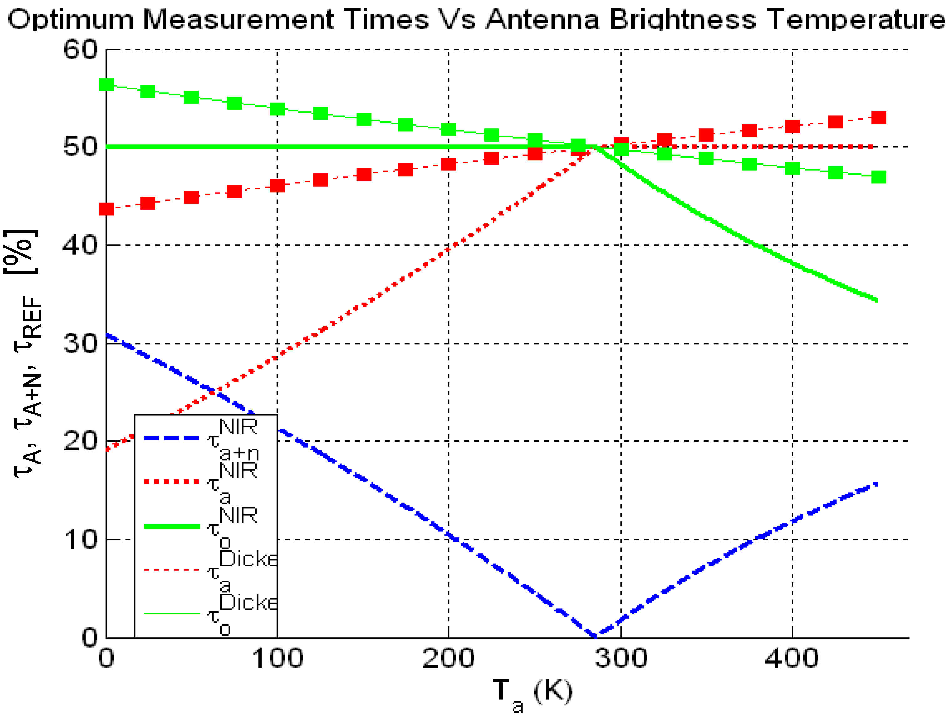
Designing and implementing a microwave radiometer with adjustable integration times for each measurement is not a complex task today thanks to digital technology. However, if—for a given application—the range of antenna temperatures is limited, a set of fixed integration times can be found that closely match the optimum performance with adjustable integration times. For the radiometer parameters listed in Section 4, Figure 8 shows the optimum integration times as a percent of the integration time. For the Dicke configuration, ${\mathsf{\tau }}_{\mathrm{A}}^{\text{Dicke}}$ and ${\mathsf{\tau }}_{\text{REF}}^{\text{Dicke}}$ values are close to the 0.5·τ (50% duty cycle) for all T_A values, which is the usual setting. For the NIR configuration, for ${\mathrm{T}}_{\mathrm{A}}\le {\mathrm{T}}_{\text{REF}}{-\mathrm{T}}_{\text{OFF}}$, ${\mathsf{\tau }}_{\text{REF}}^{\text{NIR}}$ is equal to 0.5·τ, while ${\mathsf{\tau }}_{\mathrm{A}}^{\text{NIR}}$ and ${\mathsf{\tau }}_{\mathrm{A}+\text{N}}^{\text{NIR}}$ vary significantly. However, for ${\mathrm{T}}_{\mathrm{A}}\le 120\hspace{0.17em}\text{K}$, ${\mathsf{\tau }}_{\mathrm{A}}^{\text{NIR}}$ and ${\mathsf{\tau }}_{\mathrm{A}+\text{N}}^{\text{NIR}}$ are close to 0.25·τ, which means that the noise source is switched at a rate twice higher that the latching circulator, so latching circulator control signal can be derived from the noise source control signal by a simple frequency divider.

Figure 8. Optimum measurement times (τ_REF, τ_A, τ_A+N) as a fraction of the total integration time, for the NIR and the Dicke configurations as a function of the antenna temperature (T_A [K]).

Figure 8. Optimum measurement times (τ_REF, τ_A, τ_A+N) as a fraction of the total integration time, for the NIR and the Dicke configurations as a function of the antenna temperature (T_A [K]).

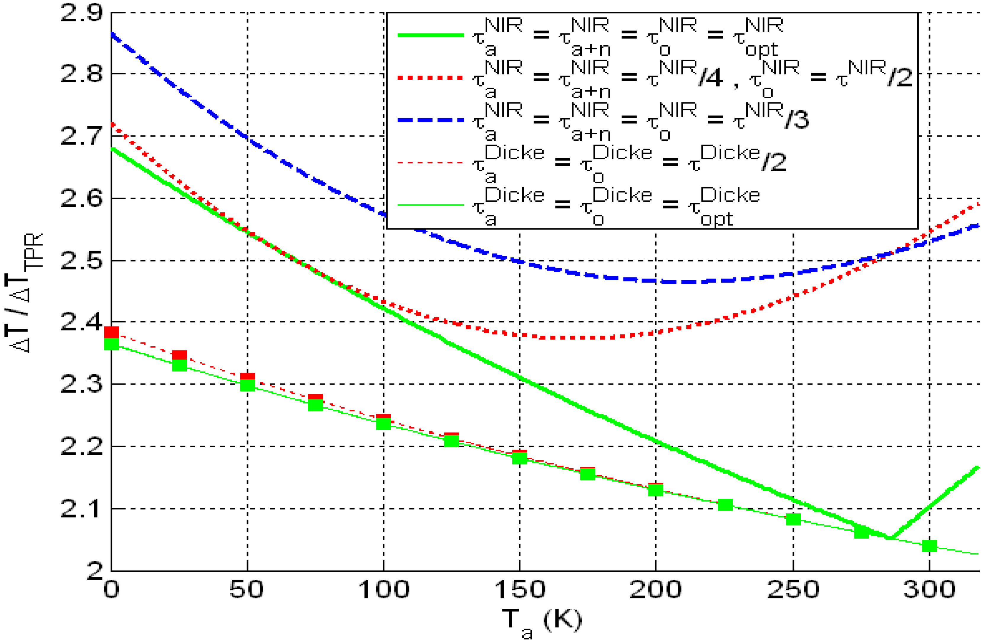
In this case, the normalized performance (relative to the ideal TPR) are shown in Figure 9. As expected, for these hardware parameters, the difference between the 50% duty cycle Dicke radiometer and the optimum Dicke performance is negligible in the whole range of T_A. For the NIR radiometer with τ_A = τ_A+N = τ_REF/2 = τ/4, the differences with the optimum NIR performance is negligible for T_A ≤ 120 K.

Figure 9. Normalized radiometric sensitivity for the NIR and the Dicke configurations as a function of the antenna temperature for optimum measurement times (continuous lines), measurement times used in this work (dashed lines) and if τ_A = τ_A+N = τ_REF = τ/3 (dotted line).

Figure 9. Normalized radiometric sensitivity for the NIR and the Dicke configurations as a function of the antenna temperature for optimum measurement times (continuous lines), measurement times used in this work (dashed lines) and if τ_A = τ_A+N = τ_REF = τ/3 (dotted line).

4. Conclusions and Further Work

Different microwave radiometer topologies have been revised in terms of their radiometric resolution and relative performance. The optimum integration times of the ultra-stable noise injection radiometer and the Dicke radiometer with duty-cycle modulation have been derived:

• The ultra-stable radiometer output does not depend on gain, receiver’s noise temperature and offset, and therefore is insensitive to drifts of these variables. The integration times have been derived as a function of the antenna temperature, the receiver’s noise temperature, and the injected noise temperature.
• The Dicke radiometer with duty-cycle modulation output depends only on receiver’s noise temperature. The integration times depend only on the antenna, reference and receiver’s noise temperatures.

In both cases, the dependence of the fractions of the integration time depends linearly with the antenna temperature.

Depending on the actual hardware parameters, the performance improvement can be significant for Dicke radiometers due to the balancing of the radiometer (~11 factor for the parameters used in this work), and more moderate (6–22%) for the ultra-stable radiometer, but these figures will be smaller if gain fluctuations are reduced.

These optimum integration times have been derived on a snapshot basis. In a real instrument, the of non-stationary effects can be mitigated by reference averaging [13,16], and for the case of the Dicke radiometer with duty-cycle modulation, by gain averaging as well [16].

The different performance and how the radiometric resolution can be improved by adjusting the integration times in the different states have been shown with an academic radiometer prototype that can be operated as TPR, Dicke or NIR. It has also been shown that in many cases, when the range of antenna temperatures to be measured is limited (in the example 0 K ≤ T_A ≤ 120 K) a set of different fixed integration times can be found that achieves a performance close to the optimum one.