Analysis of Properties of Reflectance Reference Targets for Permanent Radiometric Test Sites of High Resolution Airborne Imaging Systems

Abstract

Reliable and optimal exploitation of rapidly developing airborne imaging methods requires geometric and radiometric quality assurance of production systems in operational conditions. Permanent test sites are the most promising approach for cost-efficient performance assessment. Optimal construction of permanent radiometric test sites for high resolution airborne imaging systems is an unresolved issue. The objective of this study was to assess the performance of commercially available gravels and painted and unpainted concrete targets for permanent, open-air radiometric test sites under sub-optimal climate conditions in Southern Finland. The reflectance spectrum and reflectance anisotropy and their stability were characterized during the summer of 2009. The management of reflectance anisotropy and stability were shown to be the key issues for better than 5% reflectance accuracy.

1. Introduction

A modern information society needs reliable and up-to-date data on the environment. Exemplary applications include various monitoring and controlling processes of public authorities, societal decision-making by individual citizens, accurate measurements required to assess climate change or understand the Earth System, and the increasing sector of location-based, personal mobile applications. Geometrically and radiometrically accurate and reliable remote sensing data, ranging from global to local levels, are the basis of these applications. The principal components of accurate data are high-quality instruments and processing methods, and comprehensive testing and calibration in the laboratory. Finally, radiometric and geometric quality assurance of production systems in operational (vicarious) conditions, covering calibration, validation and characterization processes are all required to enable the most optimal and reliable utilization of the remote sensing data [1,2]. Currently, widely accepted quality assurance methods of airborne systems are missing.

This investigation concerns radiometric test sites for high-resolution, at the cm to m level, and locally operated (mostly airborne) imaging systems. Relevant instruments include multispectral photogrammetric cameras and other hyper- and multi-spectral sensors, and laser scanners. The elementary requirements of radiometric test sites are to provide targets or surfaces with traceable radiance and reflectance values and targets for point spread function (PSF) measurement [2,3,4,5,6].

High efficiency is required from the quality assurance processes to make them affordable in relevant occasions during the imaging system life cycle, especially during manufacturing, after the acquisition of the system, after changes and updates to the system (sensor, software, etc.), and during the imaging season. Permanent test sites are becoming of great interest, because they are an efficient and reliable way of conducting operational calibration and validation processes [2,7,8].

A worldwide network of permanent radiometric calibration sites by the Committee on Earth Observation Satellites (CEOS) is already available for satellite systems [9]. Ideally, a network of test sites with similar construction would be available for airborne imaging systems as well. The CEOS network is not functional for locally operated airborne imaging systems. In airborne applications the geometric test sites have mostly been emphasized. In the US, a network of geometric test sites is being developed [7]. In Europe, the idea of a European-wide test site network for geometry and radiometry has been established [8], but currently only individual test site concepts are available [10,11,12]. Existing permanent test sites for the radiometric calibration of airborne systems are the Sjökulla test site of the Finnish Geodetic Institute (FGI) in Finland (Section 3.1) [12] and the Stennis Space Center (SSC) test site in the US [3,4].

Currently, the FGI is planning to construct a new radiometric test site. As shown in our discussion in Section 2.2, one of the fundamental challenges is to find appropriate target materials. In this context, we are carrying out a controlled, comparative monitoring of the temporal performance of various potential permanent reflectance targets. We identified the reflectance spectrum and reflectance anisotropy and their stability under difficult climate conditions in Finland as central research topics. Examined materials include various gravels, and painted and unpainted concrete targets. Our objective in this investigation is to evaluate the performance of these materials using measurements carried out under laboratory conditions in 2008–2009.

We begin by presenting the theoretical foundations of reference targets for vicarious radiometric calibration in Section 2. We present the setup for the empirical investigation in Section 3 and provide the results in Section 4. Section 5 includes a discussion and recommendations.

2. Requirements for Radiometric Test Sites

2.1. Theoretical Background

An aerial camera, similar to any camera, measures brightness and the color of targets. The camera pixels are related to small areas (volumes) in the scene. The observed signal depends upon:

• the position, orientation, and movement of the camera
• the direct and diffuse sunlight reaching the observed surface
• the tilt of the surface (topography)
• the reflectance properties of the surface (or volume)
• the atmospheric absorption and scattering between the target and sensor
• the optics of the camera (lens fall-off, vignetting, stray light, diffraction, aberration, cromatisms, shutter, aperture, and so forth)
• the sensitivity of the sensor, pixel by pixel, spectrally, noise
• processing, digitalization, calibration

Of these, surface topography and reflectance are the primary quantities to extract from the data; all others are disturbances, whose effects must be minimized or corrected as much as possible. The quality is a sum of all the factors in all steps. One way to evaluate it is to use reference targets with a well-known reflectance and orientation. Below, we define more exactly how the reflectances of the targets make a signal in outdoor conditions and, based on this analysis, we derive the requirements for the radiometric calibration targets.

Figure 1. Bidirectional reflectance geometry. θ_i, ϕ_i and θ_r, ϕ_r are angles of incident and reflected light, respectively.

Figure 1. Bidirectional reflectance geometry. θ_i, ϕ_i and θ_r, ϕ_r are angles of incident and reflected light, respectively.

Assume that a (quasi-collimated) flux F₀ from the Sun at direction (θ_i, ϕ_i) is illuminating the target s. The radiation L_s(θ_r, ϕ_r) reflected to direction (θ_r, ϕ_r) can be given as [13]

$$L_s({\theta }_r,{\phi }_r)=R_s({\theta }_i,{\phi }_i,{\theta }_r,{\phi }_r)\cos ({\theta }_i)F_0({\theta }_i,{\phi }_i)$$

(1)

$R_s({\theta }_i,{\phi }_i,{\theta }_r,{\phi }_r)$ is the bidirectional reflectance factor (BRF), defined as the ratio of the radiation reflected by the target of size dA ($L_s({\theta }_i,{\phi }_i,{\theta }_r,{\phi }_r)$), to radiation reflected by an ideal white isotropic (Lambertian) reflector of the same size with similar illumination conditions ($L_{id}({\theta }_i,{\phi }_i)$):

$$R_s({\theta }_i,{\phi }_i,{\theta }_r,{\phi }_r)=\frac{L_s({\theta }_i,{\phi }_i,{\theta }_r,{\phi }_r)}{L_{id}({\theta }_i,{\phi }_i)}$$

(2)

θ_i and θ_r are illumination and reflected light (observation) zenith angles, and ϕ_i and ϕ_r are azimuth angles, as shown in Figure 1 [14,15,16]. Directional reflectance characteristics of most natural objects are highly anisotropic, and the changes in illumination and observation geometry can cause manifold differences in observed reflectance. The reference targets should be as isotropic as possible in the observation direction range of typical airborne photogrammetric and remote sensing sensors (±60°) in order to enable cost-efficient management of the anisotropy.

In normal outdoors conditions, the object reflects also diffuse radiation coming from the atmosphere, clouds and environment/adjacent objects (L_diff), and the part of the solar illumination reflects back to the sensor without reaching the object (the path radiance, L_atm). The atmosphere and aerosols between the target and observer extinct some fraction of light (e), and scatters another part towards the sensor. Symbolically, the radiation entering the sensor (L_{at_sensor}) can be given without too many details:

$$L_{at\_sensor}=e{L}_s+L_{atm}+e{L}_{diff}$$

(3)

All the quantities above depend on the wavelength (λ). In practice, other processes are involved too, but they are not significant in normal airborne imaging conditions [17].

The sensor properties define then how much and how accurately the light is sensed. The most important sensor property is the spectral sensitivity, which tells how large a fraction of each wavelength is sensed. Assuming an otherwise ideal and linear sensor, the observable signal (S_i) of each channel i can be given as:

$$S_i=B{C}_i+G_i{A}_i{\mathrm{\Omega }}_i{t}_i\underset{0}{\overset{\infty }{\int }}{f}_i(\lambda )(e(\lambda )L_s(\lambda )+L_{atm}(\lambda )+e(\lambda )L_{diff}(\lambda ))d\lambda$$

(4)

where BC_i is the black current, G_i is system gain, A_i is area of detector, Ω_i is lens solid angle, t_i is integration or exposure time, f_i(λ) is sensor spectral response and λ is wavelength. In the real world, there are more lenses, sensor and system effects, blurring, diffraction, noise, and nonlinearities, and further correction factors must be introduced, but the remaining discussion here remains the same. Angles of bi-directional geometry are not shown to simplify the equation.

At this point, the testing and validation process very much concentrates on determining how well the above equation (with the potential additional corrections) corresponds to the original target reflectance properties. The procedure can also be used to derive the calibration constants or some atmospheric properties. From Equation 4, one can see that one needs at least one dark and one bright target to determine the two coefficients, and at least one more to test the linearity. In many cases, only G_i is considered in vicarious calibration and BC_i calibration is realized by the sensor hardware; in this case, a single calibration target is sufficient.

There are at least four wavelength-dependent terms: incident light, reflectance, observation path effect, and sensor sensitivity. The spectrum of the incident light can vary in a rather large range, depending on atmospheric properties: water vapor, clouds, and especially aerosols. When the sensor band is wider than the range of incident light variations, as is typical for broadband aerial cameras, the spectral properties of the reference targets start playing a role. If R_s and F₀ vary in the same range, it can cause positive or negative interference, which is difficult to separate. The spectrum of reflectance target should be uniform to minimize the spectral interference error.

2.2. Reference Targets in Existing Radiometric Test Sites

The CEOS network of radiometric calibration sites consists of eight instrumented sites for accurate calibrations and five pseudo-invariant sites for an evaluation of the long-term stability of systems and for cross-comparison of multiple sensors [9,18]. The following have been considered as the general requirements of the surfaces of the CEOS radiometric calibration sites [6]:

• The site surface should have high spatial uniformity, relative to the pixel size. The site should also be centered in an area large enough to accommodate the sampling of a large number of pixels and to minimize the influences of atmospheric adjacency effects.
• The site should have a surface reflectance greater than 0.30 in order to provide a higher signal-to-noise ratio and reduce uncertainties due to the atmospheric path radiance.
• The surface of the site should have a flat spectral reflectance, especially to allow for the cross-calibration of multiple instruments having spectral bands with different response profiles.
• The surface properties of the site (reflectance, anisotropy, spectral) should be temporally invariant. Otherwise, adequate accuracy would be obtained only if these properties were measured for every calibration. This implies that the site should have little or no vegetation.
• The surface of the site should be horizontal and have a nearly Lambertian reflectance to minimize uncertainties due to differences in solar illumination and observation geometries. It should also be flat to minimize slope-aspect effects.
• The site should be located at a high altitude (to minimize aerosol loading and uncertainties due to the unknown vertical distribution of aerosols), far from the ocean (to minimize the influence of atmospheric water vapor), and far from urban and industrial areas (to minimize anthropogenic aerosols).
• The site should be in an arid region to minimize the probability of cloudy weather; this maximizes the probability of imaging the test site by satellite instruments and minimizes the surface reflectance changes due to soil moisture.

Requirements 1–5 are related to the geometric and radiometric properties of site surfaces, while requirements 6 and 7 are related to climate and environmental issues. The spatially and temporally uniform, high surface reflectance areas, including desert sites in North Africa, Saudi Arabia, China, Libya, Mexico, and Peru, the alkali flats, and the ice-surfaces of Greenland and Antarctica, have been studied comprehensively, in multi-year studies, to detect optimal sites [19,20,21]. The desert sand sites have shown the most stable performance [6,21].

With an airborne imaging system test site network, the requirements related to stability, location, terrain height and climate/atmospheric properties are the most difficult to realize. The most serious requirement is related to the location of the test sites. Ideally, test site should be located within a 300 km (1 h) radius of the base stations for survey aircrafts [8]. The presumption is that the test sites have to be built in a sub-optimal environment, which includes such meteorological conditions as rain, dust, pollutions, salinity, snow, frost, heat, or sunshine. The test site should be operational during the imaging season, which typically extends from April to September in Europe [22], but is expected to increase with the new digital imaging sensors.

The SSC test site has concrete and painted concrete targets with a reflectance range of approximately 0.05–0.50 [3]. At the Sjökulla test site, the permanent reflectance and spatial resolution targets are constructed out of gravel and have a reflectance range of 0.05–0.50 as well (Figure 2) [12,23]. The CEOS satellite test sites are bright, large Earth surfaces: sand deserts, dry lakebeds and Antarctica Ice targets [18]. Permanent devices for the in situ measurement of the atmospheric and surface reflectance properties exist in the CEOS test sites intended for the absolute radiometric calibration and in the SSC test site.

The stability issues have been studied especially with CEOS sites; they have shown stable reflectances of better than 5%. The test sites in less optimal conditions have shown daily, seasonal and cyclic changes in reflectance properties [23,24,25,26]. For example, the mature (60 year old) concrete surfaces at the military airfield on Thorney Island in England have shown that reflectance factors have varied by a factor of two during the year, and are highly influenced by biological materials growing over surfaces and their interactions with moisture [26]. At Sjökulla, the gravel targets have shown many advantages, including durability, low maintenance efforts, natural cleaning of the surface by rain, and a fast drying process, but also significant temporal changes [12,23,27].

In the non-ideal conditions, the complete radiative transfer must be accounted for both in the design of materials and in instrumentation for the intended spatial, angular and spectral ranges. The design of durable, stable, spatially uniform, permanent, open-air reference targets become the central question to be solved. Getting better understanding of the performance of various potential materials is the objective of our investigation.

3. Materials and Methods

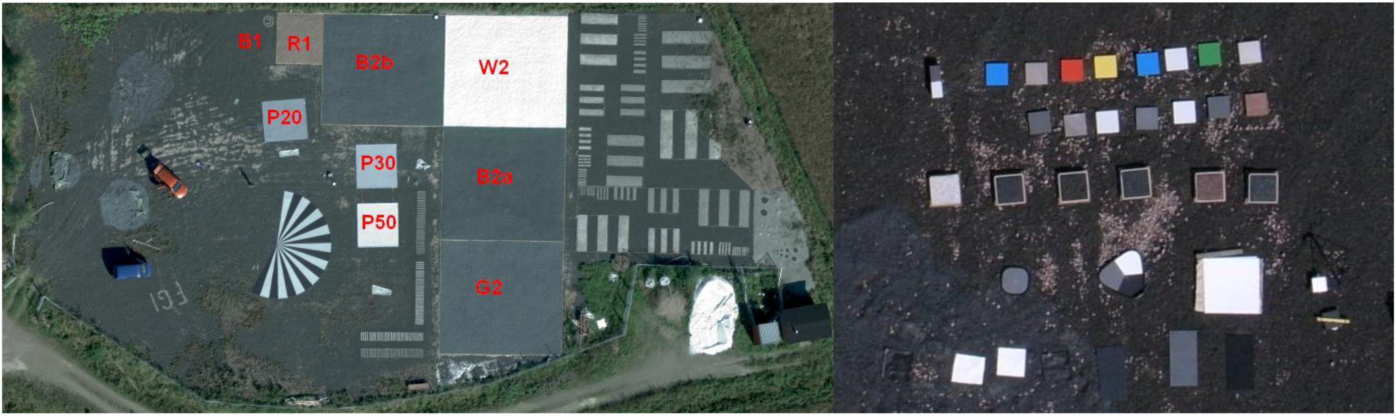
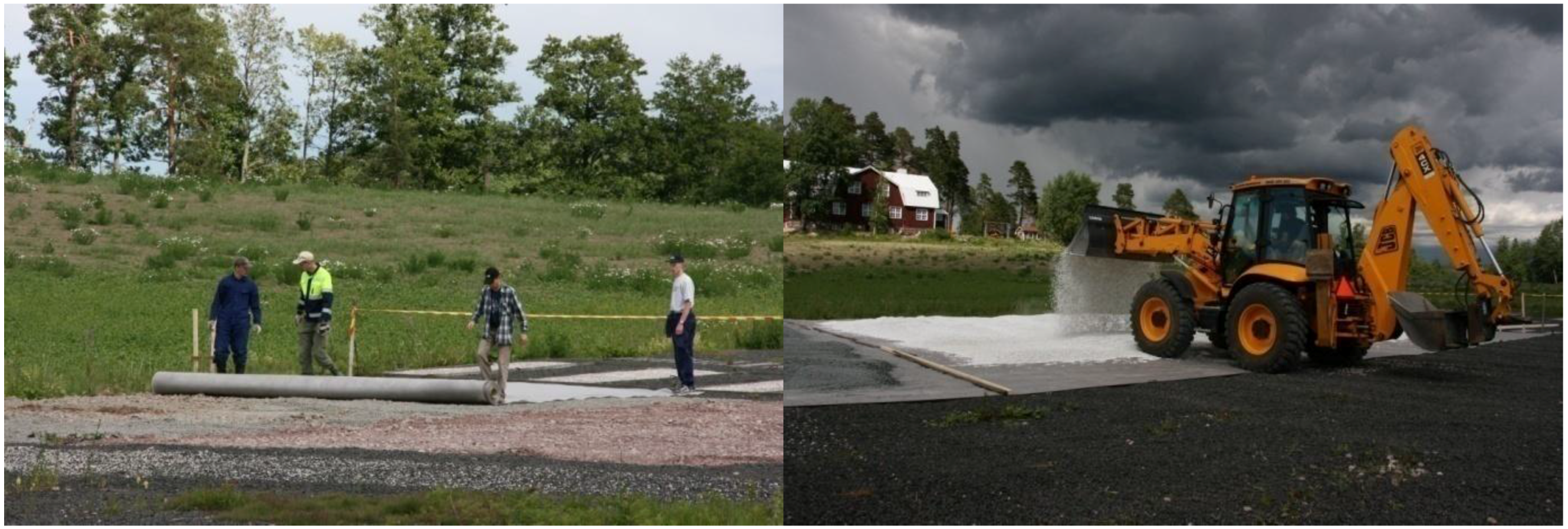
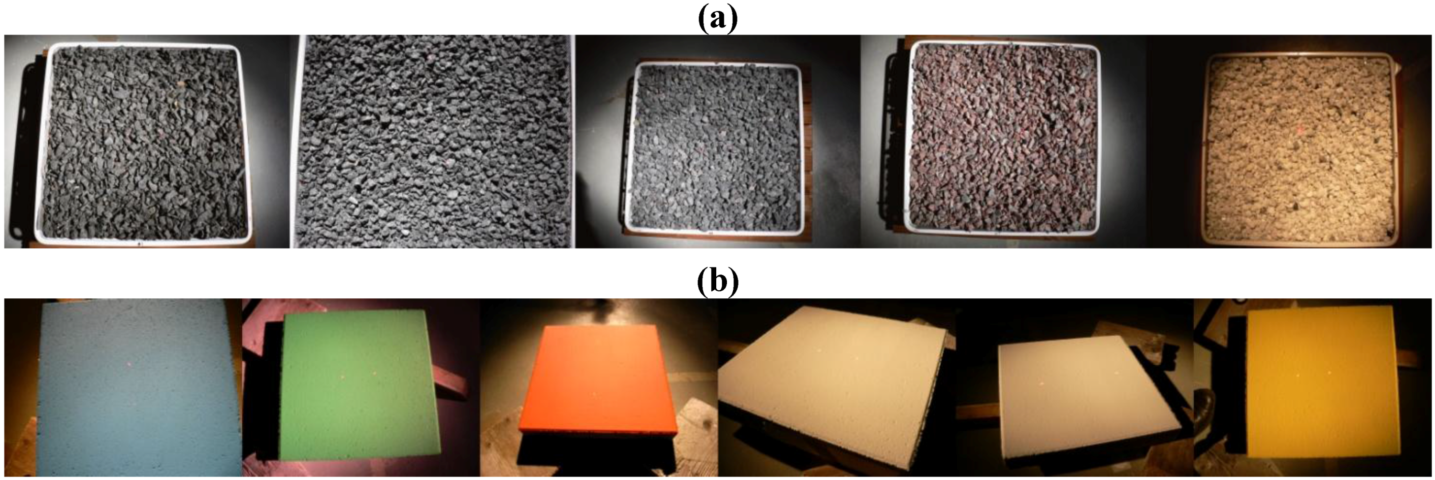
3.1. Reflectance Targets

The FGI constructed the Sjökulla test site (60°14′31, 24°23′1) in 1993 [12,27]. The test site contains reflectance targets for radiometric calibration and edge and bar targets for PSF measurements (Figure 2). It is located in the countryside and surrounded by agricultural parcels. The test site suffers occasionally from dust and pollen from the environment, cloudy weather, and traffic regulations for the main Helsinki airport. Sjökulla is located in Southern Finland, approximately 20 km from the coastline of the Gulf of Finland. The area has a humid continental climate, characterized by four seasons and a large seasonal temperature variance. Summers are warm and humid and winters are cold with persistent snow cover. The yearly temperature variation can be −30 to 30 °C.

We renovated the test site completely in the summer of 2008. Now there are six reflectance targets made of homogeneous gravel. Two smaller squares of black gabro (B1) and red granite (R1), measuring 6 m by 6 m, date from the original construction in 1993. Larger rectangles 14 m by 15 m in size were constructed using new materials: two similar black granites (B2a, B2b), grey granite (G2) and white limestone (W2). All gravels form at least a 5 cm thick layer above the strong root-blocking carpet (Figure 3). Originally, the stones were covered by fine powder. We cleaned them using strong water showers. Rain water has cleaned more of them, but some remnants of dust still remained, especially on the inner stones, and expressed themselves when turning the stones and dragging the surface. For reference and measurement purposes, we filled small transportable boxes, 0.5 m × 0.5 m in size, with the same gravel (Figure 4a). We keep these outside in conditions similar to those of the test site and bring then to laboratory only during measurements.

Figure 2. Left: Permanent Sjökulla image quality test field in September 2008 (with reference target indicators; P20, P30 and P40 are non-permanent targets). Right: Reference target samples at the test site in summer 2009. Colors and brightness are not calibrated or adjusted to the same scale.

Figure 2. Left: Permanent Sjökulla image quality test field in September 2008 (with reference target indicators; P20, P30 and P40 are non-permanent targets). Right: Reference target samples at the test site in summer 2009. Colors and brightness are not calibrated or adjusted to the same scale.

Figure 3. Construction of a test field of gravel. The root blocking carpet is installed (left) and a 5–10 cm layer of gravel spread over it (right).

Figure 3. Construction of a test field of gravel. The root blocking carpet is installed (left) and a 5–10 cm layer of gravel spread over it (right).

To test other alternative materials and coatings, we purchased a set of concrete tiles, 40 cm × 40 cm in size, from a hardware store (Figure 4b). We painted the tiles using a full-matt, alkali-resistant, acrylate socle paint, Yki of Tikkurila, mixed with dark grey, white, blue, green, red and yellow paint pigments. Also, we evaluated unpainted red and grey concrete tiles.

Figure 4. Examples of various target types. (a) Gravel targets of size 50 cm × 50 cm. From left: B1, B2a, G2, R1, W2. (b) Painted concrete targets of size 40 cm × 40 cm. From left: blue, green, red, white, grey and yellow. Colors and brightness are not calibrated or adjusted to the same scale.

Figure 4. Examples of various target types. (a) Gravel targets of size 50 cm × 50 cm. From left: B1, B2a, G2, R1, W2. (b) Painted concrete targets of size 40 cm × 40 cm. From left: blue, green, red, white, grey and yellow. Colors and brightness are not calibrated or adjusted to the same scale.

We selected promising materials for the monitoring experiment, taking into account their technical feasibility, expected behavior and spectral properties especially in the visible to near infrared spectral range. Details of the evaluated materials are given in Table 1.

Table 1. Details of targets, measurement dates and illumination zenith angles. For all targets, the year it was established is given. For gravels, the type and grain size are given. For painted tiles, the tile type, paint type and number of paint layers are given. When more than one illumination height was used the underlined data was analyzed, unless otherwise mentioned. Wet: wet target.

Description	Measurement dates and illumination zenith angles (°)
Gravel
B1: Black gabbro from Hyvinkää, 8–16 mm, 1993	28.10.2008: 26.4°, 44.9°, 69.4°; 5.5.2009: 46°, 65°; 3.8.2009: 48.2°; 25.9.2009: 50.5°
B2a: Black gabbro from Hyvinkää, 4–12 mm, 2008	28.10.2009: 26.5°, 46.8°, 68°; 5.5.2009: 45.1°, 65.1°; 3.8.2009: 48.2°; 25.9.2009: 50.5°
B2b: Same as B2a	28.10.2009: 26.5°, 46.8°, 68°; 5.5.2009: 45.1°, 65.1°; 3.8.2009: 48.2°; 25.9.2009: 50.5°
B2b_wet	25.9.2009: 50.5°
G2: Gray granite from Hyvinkää Harumäki, 8–16 mm, 2008	28.10.2008: 26.8°, 44.8°, 69.1°; 5.5.2009: 45°, 65.5°; 3.8.2009: 48.2°; 25.9.2009: 50.5°
G2_wet	25.9.2009: 50.5°
R1: Red granite from Ridasjärvi, 8–16 mm, 1993	28.10.2008: 26.9°, 45.4°, 68.9°; 5.5.2009: 44.8°, 65.3°; 3.8.2009: 48.2°; 25.9.2009: 50.5°
R1_wet	25.9.2009: 50.5°
W2: White lime stone from Parainen, 8–16 mm, 2008	28.10.2008: 26.2°, 45.5°, 68.9°; 5.5.2009: 44.8°, 65.3°; 3.8.2009: 48.2°; 25.9.2009: 50.5°
W2_wet	25.9.2009: 50.5°
Unpainted concrete tiles
T_R: Red concrete tile, grooves, 2009	10.3.2009: 58.5°; 03.08.2009: 58.4°; 25.9.2009: 57.5°
T_G1: Unpainted grey tile, 2009	10.3.2009: 58.1°; 03.08.2009: 58.4°; 25.9.2009: 57.5°
T_G1_wet	25.9.2009: 57.5°
T_G2: Unpainted grey tile, 2009	10.3.2009: 58.5°; 3.8.2009: 58.4°; 25.9.2009: 57.5°
Painted grey and white concrete tiles
PT_G1: T_G2, Grey TVT 4991, 2 layers, 2009	10.3.2009: 58.5°; 3.8.2009: 58.4°; 25.9.2009: 57.5°
PT_G2: T_G2, Grey TVT 4991, 1 layer, 2009	10.3.2009: 58.5°; 3.8.2009: 58.4°; 25.9.2009: 57.5°
PT_W1: T_G2, White TVT 6500, 2 layers, 2009	4.3.2009: 58.4°; 3.8.2009: 58.4°; 25.9.2009: 57.5°
PT_W1_wet	25.9.2009: 57.5°
PT_W2: T_G2, White TVT 4986, 2 layers, 2009	4.3.2009: 58.4°; 3.8.2009: 58.4°; 25.9.2009: 57.5°
PT_W3: T_G2, White TVT 4986, 1 layer, 2009	10.3.2009: 58.5°; 3.8.2009: 58.4°; 25.9.2009: 57.5°
Painted color concrete tiles
PT_B: T_G2, Blue TVT L358, 2 layers, 2008	4.3.2009: 58.4°; 3.8.2009: 58.4°; 25.9.2009: 57.5°
PT_G: T_G2, Green TVT L380, 1 layer, 2009	4.3.2009: 58.4°; 3.8.2009: 58.4°; 25.9.2009: 57.5°
PT_R: T_G2, Red TVT M320, 3 layers, 2009	4.3.2009: 58.4°; 3.8.2009: 58.4°; 25.9.2009: 57.5°
PT_Y: T_G2, Yellow TVT K302, 2009	4.3.2009: 58.4°; 3.8.2009: 58.4°; 25.9.2009: 57.5°

Table 1. Details of targets, measurement dates and illumination zenith angles. For all targets, the year it was established is given. For gravels, the type and grain size are given. For painted tiles, the tile type, paint type and number of paint layers are given. When more than one illumination height was used the underlined data was analyzed, unless otherwise mentioned. Wet: wet target.

Description	Measurement dates and illumination zenith angles (°)
Gravel
B1: Black gabbro from Hyvinkää, 8–16 mm, 1993	28.10.2008: 26.4°, 44.9°, 69.4°; 5.5.2009: 46°, 65°; 3.8.2009: 48.2°; 25.9.2009: 50.5°
B2a: Black gabbro from Hyvinkää, 4–12 mm, 2008	28.10.2009: 26.5°, 46.8°, 68°; 5.5.2009: 45.1°, 65.1°; 3.8.2009: 48.2°; 25.9.2009: 50.5°
B2b: Same as B2a	28.10.2009: 26.5°, 46.8°, 68°; 5.5.2009: 45.1°, 65.1°; 3.8.2009: 48.2°; 25.9.2009: 50.5°
B2b_wet	25.9.2009: 50.5°
G2: Gray granite from Hyvinkää Harumäki, 8–16 mm, 2008	28.10.2008: 26.8°, 44.8°, 69.1°; 5.5.2009: 45°, 65.5°; 3.8.2009: 48.2°; 25.9.2009: 50.5°
G2_wet	25.9.2009: 50.5°
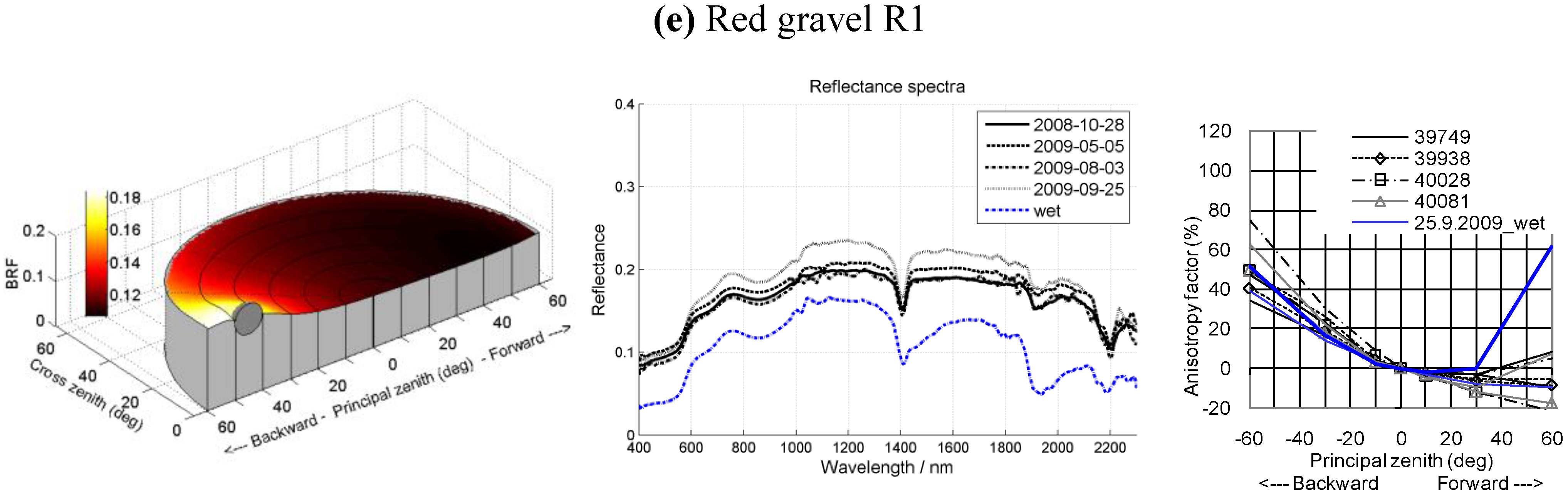
R1: Red granite from Ridasjärvi, 8–16 mm, 1993	28.10.2008: 26.9°, 45.4°, 68.9°; 5.5.2009: 44.8°, 65.3°; 3.8.2009: 48.2°; 25.9.2009: 50.5°
R1_wet	25.9.2009: 50.5°
W2: White lime stone from Parainen, 8–16 mm, 2008	28.10.2008: 26.2°, 45.5°, 68.9°; 5.5.2009: 44.8°, 65.3°; 3.8.2009: 48.2°; 25.9.2009: 50.5°
W2_wet	25.9.2009: 50.5°
Unpainted concrete tiles
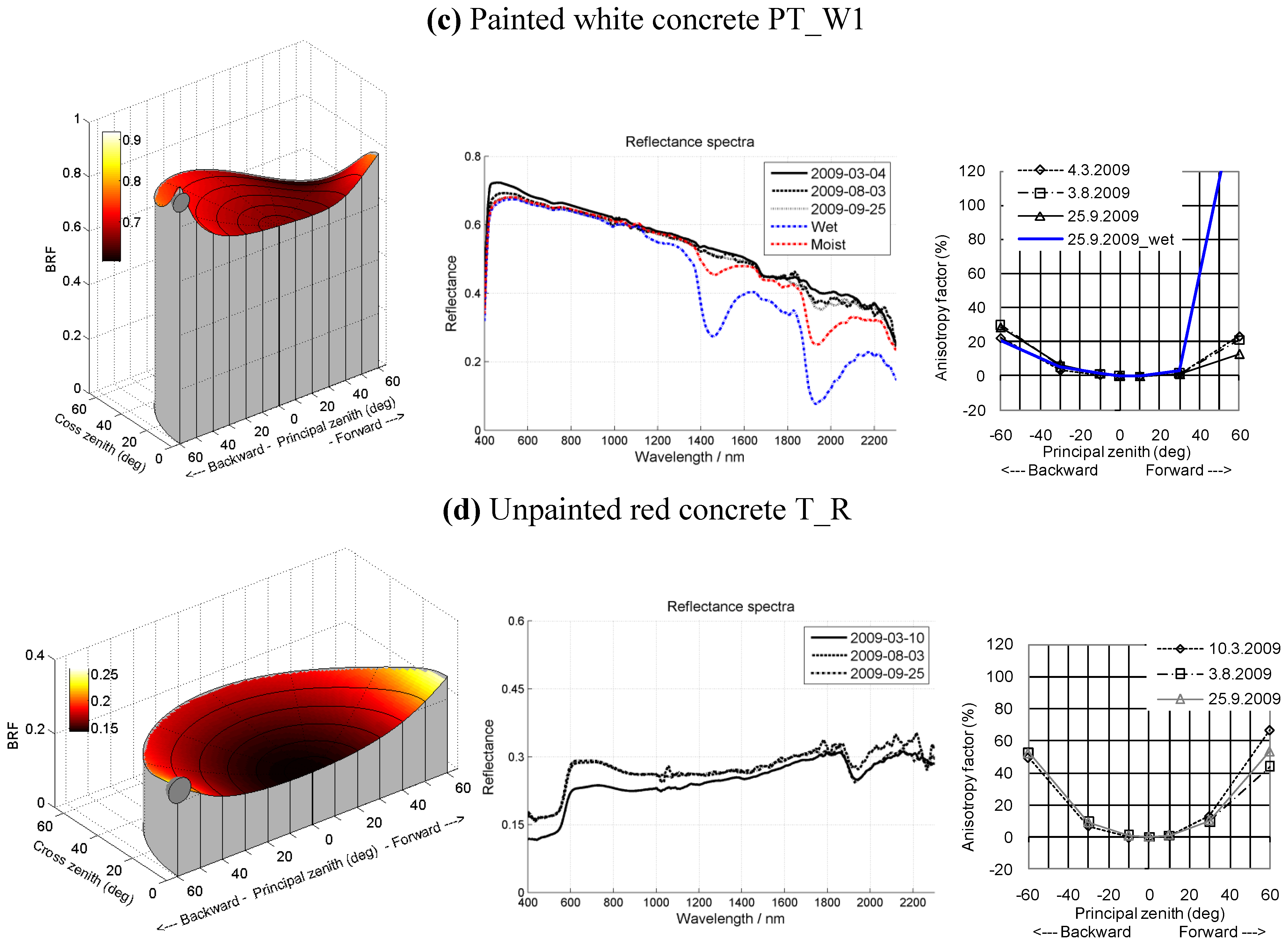
T_R: Red concrete tile, grooves, 2009	10.3.2009: 58.5°; 03.08.2009: 58.4°; 25.9.2009: 57.5°
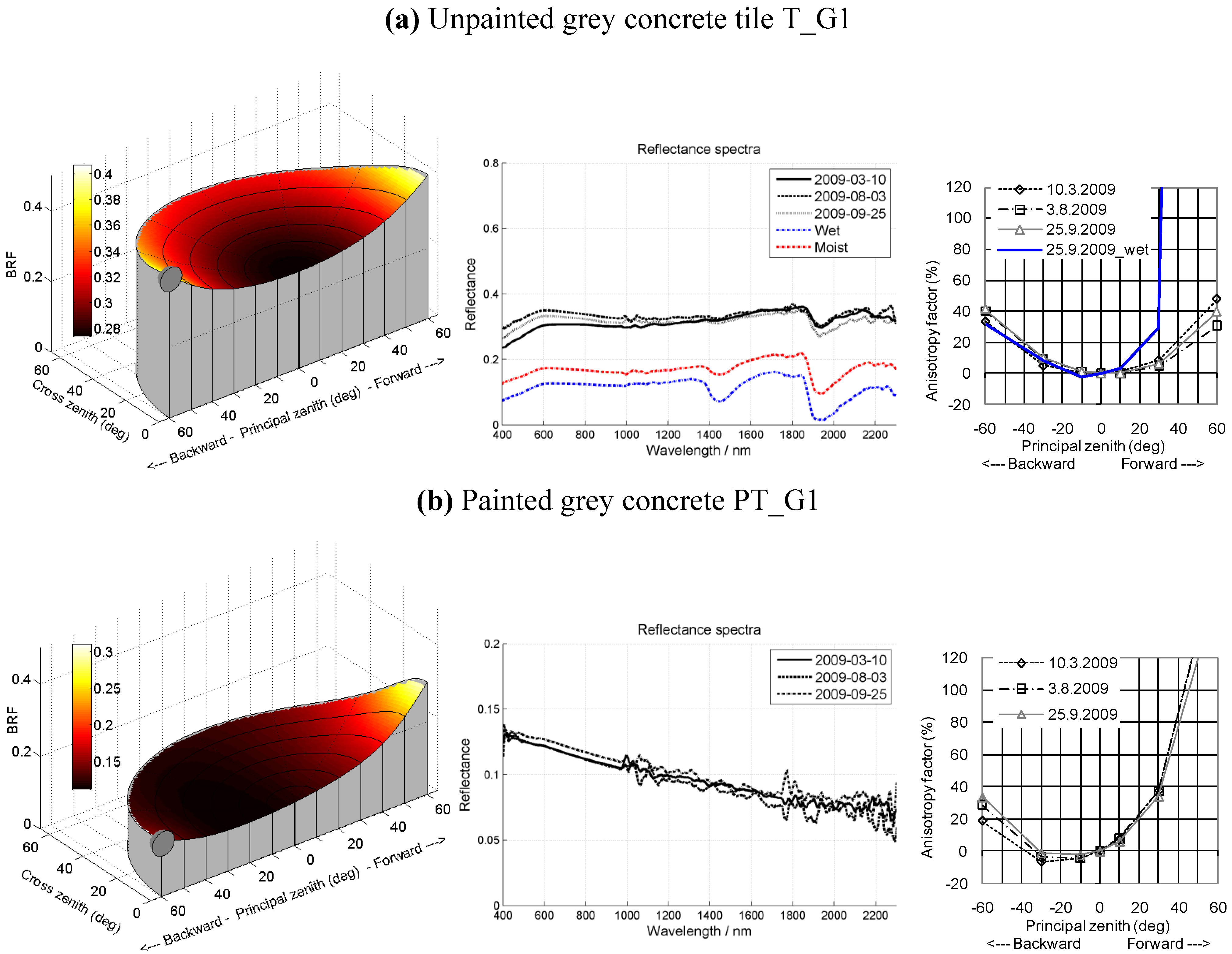
T_G1: Unpainted grey tile, 2009	10.3.2009: 58.1°; 03.08.2009: 58.4°; 25.9.2009: 57.5°
T_G1_wet	25.9.2009: 57.5°
T_G2: Unpainted grey tile, 2009	10.3.2009: 58.5°; 3.8.2009: 58.4°; 25.9.2009: 57.5°
Painted grey and white concrete tiles
PT_G1: T_G2, Grey TVT 4991, 2 layers, 2009	10.3.2009: 58.5°; 3.8.2009: 58.4°; 25.9.2009: 57.5°
PT_G2: T_G2, Grey TVT 4991, 1 layer, 2009	10.3.2009: 58.5°; 3.8.2009: 58.4°; 25.9.2009: 57.5°
PT_W1: T_G2, White TVT 6500, 2 layers, 2009	4.3.2009: 58.4°; 3.8.2009: 58.4°; 25.9.2009: 57.5°
PT_W1_wet	25.9.2009: 57.5°
PT_W2: T_G2, White TVT 4986, 2 layers, 2009	4.3.2009: 58.4°; 3.8.2009: 58.4°; 25.9.2009: 57.5°
PT_W3: T_G2, White TVT 4986, 1 layer, 2009	10.3.2009: 58.5°; 3.8.2009: 58.4°; 25.9.2009: 57.5°
Painted color concrete tiles
PT_B: T_G2, Blue TVT L358, 2 layers, 2008	4.3.2009: 58.4°; 3.8.2009: 58.4°; 25.9.2009: 57.5°
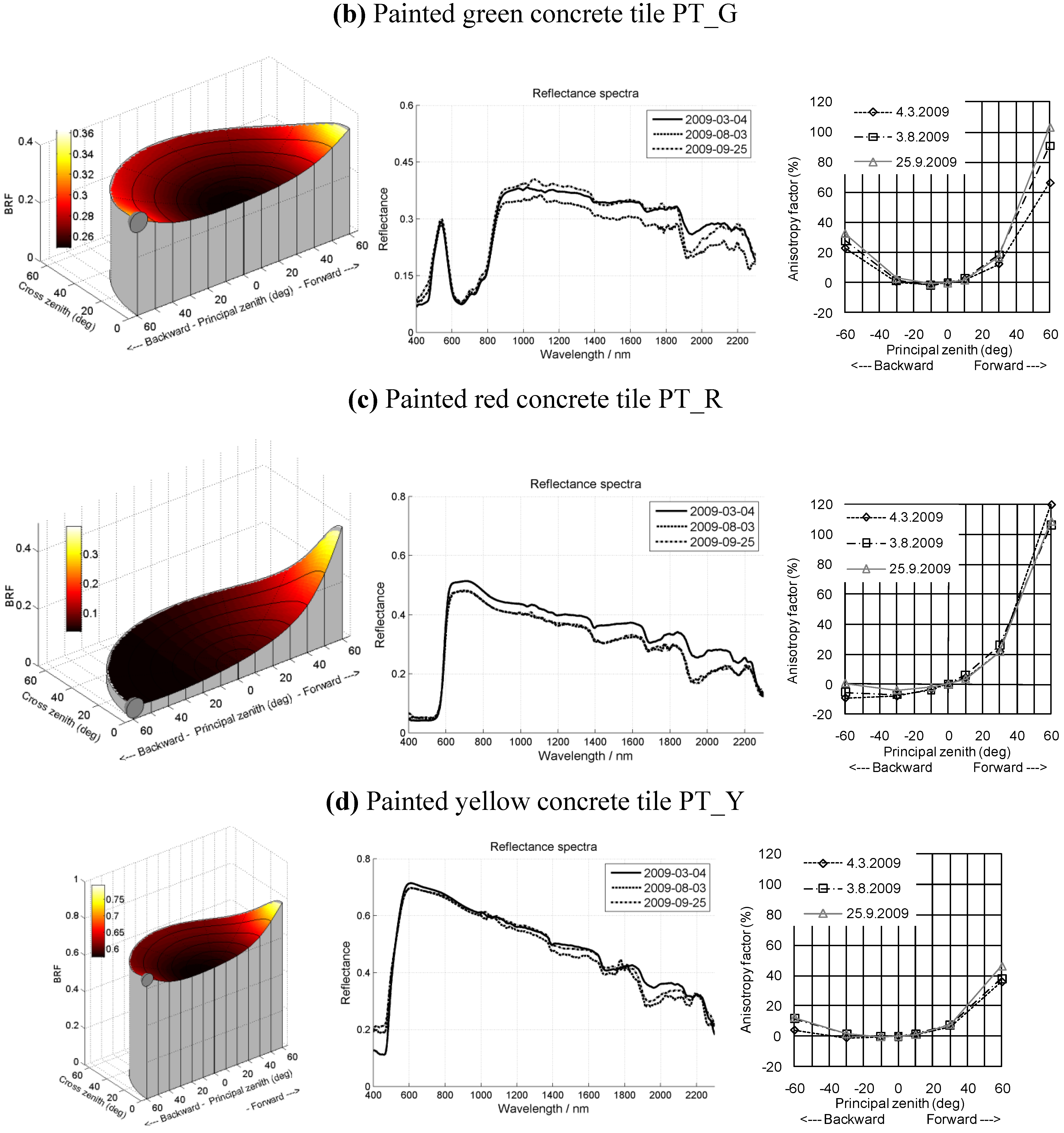
PT_G: T_G2, Green TVT L380, 1 layer, 2009	4.3.2009: 58.4°; 3.8.2009: 58.4°; 25.9.2009: 57.5°
PT_R: T_G2, Red TVT M320, 3 layers, 2009	4.3.2009: 58.4°; 3.8.2009: 58.4°; 25.9.2009: 57.5°
PT_Y: T_G2, Yellow TVT K302, 2009	4.3.2009: 58.4°; 3.8.2009: 58.4°; 25.9.2009: 57.5°

3.2. Reflectance Measurements

We measured the BRFs of the test targets several times in 2008 and 2009. The measurements were mostly taken at the FGI laboratory in Masala, using a Finnish Geodetic Institute field goniospectrometer (FIGIFIGO). We have also measured the old gravels using several other goniospectrometers since 1993 [23].

FIGIFIGO is a lightweight portable instrument for measurement of the BRF of surfaces either in the field or in the laboratory. It consists of a casing, containing an ASD FieldSpec Pro FR spectrometer (Analytical Spectral Devices, Boulder, CO, USA) and assisting electronics, and a turning arm housing the spectrometer optics. A sample is positioned in front of the device and the arm is turned over the sample measuring the reflected radiance from a series of zenith angles. To measure reflectance in full hemisphere, the device is rotated around the sample and the zenith turn sequence repeated from 4 to 10 azimuth angles. Please see [16] for a more detailed description of the device and the measurement sequence. The fore optics used in the presented measurements have a footprint of about 10 cm in diameter on sample in nadir measurement. The usable spectral range in the measurements is from 400 to 2,300 nm.

In the laboratory, the light source was an Oriel quarz-tungsten-halogen Research Light with a power of 1,000 W. The light is collimated using an off-axis parabolic mirror with a diameter of 50 cm. The angle of incidence can be freely set between 15 and 80 degrees. We calibrated the measurements using Labsphere Spectralon panels. The accuracy of the BRF measurements of uniform targets in laboratory conditions is clearly better than 5% [16].

We measured the targets in the spring, summer and autumn of 2009 to get information about their temporal stability. Usually, we measured the BRFs over the full hemisphere, but in some cases we only measured the principal plane (the plane in which the illumination source, the target, and the nadir of the target are; the principal plane typically shows the most distinct characteristics of the anisotropy). We measured the gravel targets using 45–50° illumination zenith angles. The influence of illumination height was characterized in 2008 using illumination zenith angles of 26°, 45° and 69°. We measured the concrete targets using illumination zenith angle of approximately 58°. Details of the measurements are given in Table 1.

We evaluated the influence of moisture on the gravel targets B2b, G2, R1 and W2, the unpainted concrete tile, and the concrete tile painted with white paint (Table 1). First, we measured the BRFs of dry targets. Then, we sprayed targets with water. In the case of gravel targets, we measured the reflectance spectrum over the entire hemisphere once and, in the cases of concrete targets, the measurement over the principal plane was carried out a few times during the drying period.

We assessed the spectral uniformity by evaluating reflectance spectrums and by calculating peak-to-peak variation coefficients (C_{peak_to_peak}) in 50 nm windows over the spectrum at nadir:

C_{peak_to_peak} = 100*(R_max − R_min)/R_average [%]

(5)

where R_max, R_min and R_average are the maximum, minimum and average reflectance in the measurement window, respectively.

We characterized anisotropy using the BRFs over the hemisphere and with anisotropy factors (F_anisotropy):

F_anisotropy = 100*(R_{off_nadir} − R_nadir)/R_nadir [%]

(6)

where R_nadir is the reflectance in the nadir direction and R_{off_nadir} is the reflectance in the off-nadir direction, which is being evaluated. We mostly evaluated the anisotropy of the principal plane in the nadir direction (observation zenith angles 0 and ±10°), in FOV of typical photogrammetric imaging sensors (±30°) and in FOV of special multi-angular imaging systems (±60°).

We assessed the relative differences (changes) of reflectance factors (R_diff) by

R_diff = 100*(R − R _ref)/R _ref [%]

(7)

where R _ref is the reference value and R is the measurement being evaluated.

4. Results

We present the measurement results in Figure 5, Figure 6 and Figure 7. On the left section in the figures, the 3D plots depict the anisotropy of BRF on the green band (550 ± 25 nm), i.e., the plots show the reflectance as a function of observation direction; x-axis is the observer zenith angle at the solar principal plane (principal zenith); y-axis is the observer zenith angle at the plane perpendicular to the solar principal plane (cross zenith); z-axis is the BRF; a left-right symmetry is assumed. The observation directions in the illumination direction are called backward direction and the observation directions opposite to illumination direction are called forward direction. The front edge of the 3D plot shows the reflectance factor in the solar principal plane. The gray ball is positioned in direction of the direct backscatter, where no data is available due to instrument self-shadowing. On the middle section in the figures, reflectance spectra at the nadir observation direction are given for each measurement time. On the right section in the figures, anisotropy factor (Equation 6) on the panchromatic (PAN) channel is depicted in the solar principal plane at observer zenith angles of 0°, ±10°, ±30° and ±60° for each measurement time.

The major analysis was performed over blue (B: 435–485), green (G: 535–585 nm), red (R: 610–660 nm), near infrared (NIR: 835–885 nm) and PAN (450–950 nm) channels; the spectrums on short wave infrared (SWIR: 1,000–2,200 nm) is presented only in Figure 5, Figure 6 and Figure 7. Most of the analysis concerns spectrally uniform targets (grey, black, white), but we also present the results from the color targets.

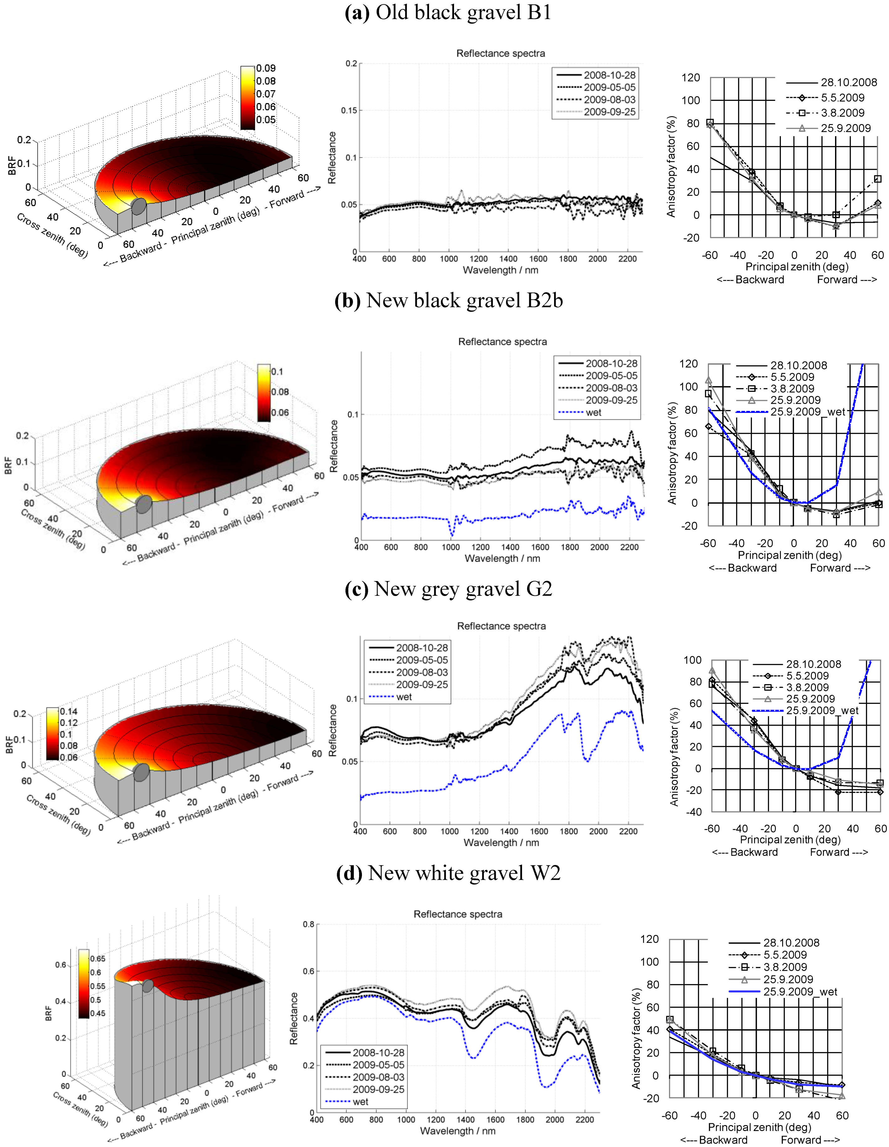
4.1. Spectrum

The spectra of the test targets taken from nadir are shown in Figure 5, Figure 6 and Figure 7, in the middle sections. Basically, the flatter the spectrum the better, except for the fact that color targets will show color. The spectra are shown in full measured range, but most users need only the visible to NIR (VIS-NIR) range, which is about 400–1,000 nm.

The old black gravel (B1) had a rather uniform spectrum, and the new black gravel (B2b) was very close (Figure 5a,b). New grey gravel (G2) was also acceptable in VIS-NIR, but brightened in longer wave infrared. New white gravel (W2) had some curvature, but was still mostly adequate. Unpainted gray concrete (T_G1) was excellent, except for a small drop in blue (Figure 6a). The painted grey and white tiles had a decreasing trend that needs attention when used (Figure 6b,c). The colored tiles had all their specific patterns, which must be taken into account when used (Figure 7).

Peak-to-peak variation (not shown in figures, but can be derived from spectrums) (Equation 5) was less than 5–10% on the PAN channel for grey targets; an exception to this pattern was the unpainted grey concrete tile, for which the reflectance increased relatively steeply up to 600 nm. For all measurements, some noise appeared in the ultraviolet-blue region because ASD spectrometer is rather inaccurate in the 350–500 nm range. The average reflectances (over the PAN spectrum) of the black, grey and white gravels were approximately 0.05, 0.07 and 0.50, respectively. The average reflectances were approximately 0.12 for painted grey targets, 0.60 for painted white targets and 0.20 and 0.30 for the two unpainted concrete tiles.

The properties of the three different red targets (gravel, tile, painted tile) can be compared. The painted red tile had the sharpest and most uniform edge at approximately 600 nm, ranging from a 0.05 to a 0.45 reflectance (Figure 7c). The corresponding step for red concrete produced a range of 0.15 to 0.30 and was relatively sharp (Figure 6d), whereas for red gravel it produced a range of 0.10 to 0.15 and was blunt (Figure 5e). The red gravel was the least favorable for calibration purposes.

Figure 5. Reflectance characterization of gravels (a) B1, (b) B2b, (c) G2, (d) W2 and (e) R1. Left: The BRF of the green channel (550 ± 25 nm). Middle: the spectra at nadir at different measurement times. Right: Anisotropy factors (Equation 6) at the principal plane at different measurement times. Further details of diagrams are given in the text.

Figure 5. Reflectance characterization of gravels (a) B1, (b) B2b, (c) G2, (d) W2 and (e) R1. Left: The BRF of the green channel (550 ± 25 nm). Middle: the spectra at nadir at different measurement times. Right: Anisotropy factors (Equation 6) at the principal plane at different measurement times. Further details of diagrams are given in the text.

Figure 6. Reflectance characterization of concrete tiles: (a) unpainted grey T_G1, (b) painted grey PT_G1, (c) painted white PT_W1 and (d) unpainted red T_R, as in Figure 5.

Figure 6. Reflectance characterization of concrete tiles: (a) unpainted grey T_G1, (b) painted grey PT_G1, (c) painted white PT_W1 and (d) unpainted red T_R, as in Figure 5.

Figure 7. Reflectance characterization of concrete targets (a) blue PT_B, (b) green PT_G, (c) red PT_R and (d) yellow PT_Y, as in Figure 5.

Figure 7. Reflectance characterization of concrete targets (a) blue PT_B, (b) green PT_G, (c) red PT_R and (d) yellow PT_Y, as in Figure 5.

4.2. Reflectance Anisotropy

All the gravel targets were strong backward scatterers (Figure 5) with a moderate bowl shape. With a 45–50° illumination zenith angle, the anisotropy factors were approximately 40–100%, 20–40%, and less than 10% at the principal plane for the observer zenith angles of 60°, 30° and 10° in the backward direction, respectively. The gravel targets were in many cases darker in the forward direction than at nadir; the anisotropy factors were −20–30%, −15–20% and less than −5% at the principal plane for the observer zenith angles of 60°, 30° and 10°, respectively. The general bi-directional reflectance characteristic of black and grey gravels was similar (Figure 5a–c) and the anisotropy was higher than on the white gravel (Figure 5d). The white gravel was the closest to being usable.

The unpainted grey and red concrete targets had a rather symmetric bowl-shaped BRF (Figure 6a,d). With an illumination zenith angle of about 58°, the anisotropy factors were approximately 30–60%, less than 10% and less than 5% at principal plane for the observer zenith angles of ±60°, ±30° and ±10°, respectively. These are clearly the best of all those which we tested.

The painted tiles were all more or less forward scatterers. The brightest ones were the most isotropic and darkest ones the most anisotropic. For the concrete tile with a grey paint, the anisotropy factor was greater than 100–180%, 40% and less than 10% at the 60°, 30° and 10° forward direction at the principal plane with a 57° illumination zenith angle, respectively; in the backward direction the anisotropy factors were 20–40%, less than −5% and less than −5%, respectively, for the corresponding zenith angles. The white painted tiles had a bowl-shaped BRF with anisotropy factors of approximately 20–40%, 5% and less than 2%, in the 60°, 30° and 10° forward and backward observer directions (Figure 6c). The figures were similar with colored tiles, and one has to note that different colors have differing anisotropies.

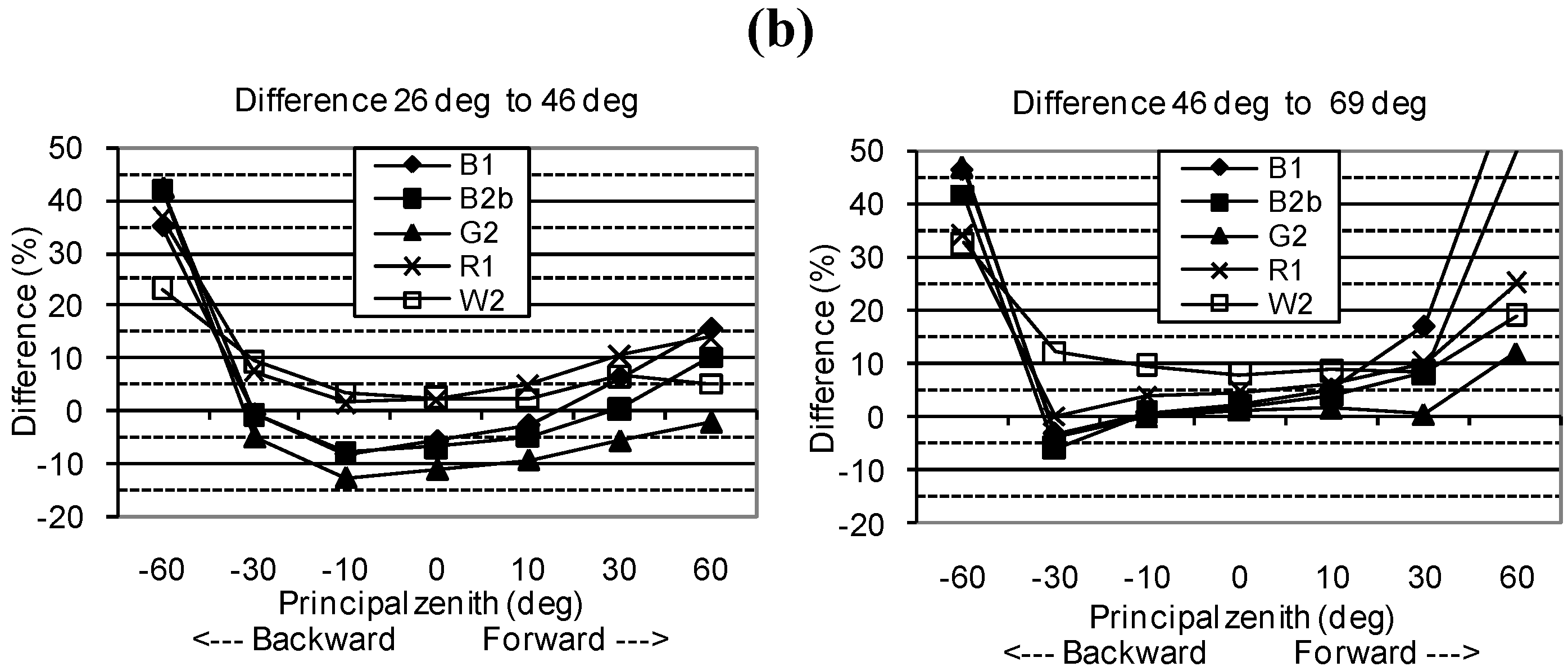
4.3. Influences of the Illumination Zenith Angle

We evaluated the influence of the illumination height on the gravel targets using approximately 26°, 46° and 69° illumination zenith angles (Figure 8).

Figure 8. Influence of illumination height (zenith angles 26° 46° and 69°) on reflectance factors. (a) 3-D BRF plots of black (B2b) (top) and white (W2) (bottom) gravels on green channel (550 ± 25 nm). (b) Relative differences of measurements with 26° and 46° (left) and 46° and 69° (right) illumination zenith angles on the PAN channel at the principal plane (Equation 7; the measurement with smaller illumination zenith angle was used as a reference).

Figure 8. Influence of illumination height (zenith angles 26° 46° and 69°) on reflectance factors. (a) 3-D BRF plots of black (B2b) (top) and white (W2) (bottom) gravels on green channel (550 ± 25 nm). (b) Relative differences of measurements with 26° and 46° (left) and 46° and 69° (right) illumination zenith angles on the PAN channel at the principal plane (Equation 7; the measurement with smaller illumination zenith angle was used as a reference).

All gravel targets behaved rather similarly. The most significant observation was that the bowl shape increased as the zenith angle of illumination increased, that is to say, forward, backward, and sideways scattering increased (Figure 8a). The smallest differences were near the nadir observation direction (observer zenith angles of 0 to ±30°): the reflectance either increased or decreased approximately 5 to 10%, depending on the target (Figure 8b). The differences rose on the 60° backward direction, typically to 25–50%. On the 60° forward direction, the differences were mostly lower than that; but on black gravels B1 and B2b they were higher.

White and red gravels appeared brighter as the illumination zenith angle decreased (Figure 8b). The behavior of black and grey gravels was opposite near the nadir observation directions. With low observation directions (±60°), all targets appeared brighter with a decreasing illumination zenith angle.

Multi-illumination measurements have not been taken for the concrete targets, but based on the gravel and 100 other targets in the BRF database, a similar trend is expected.

These results indicated that the small differences in illumination heights (zenith angles 45–50°) in the measurements of gravels do not influence the analysis for up to ±30° observer zenith angels, and that the results are also representative in comparison to the results for concrete targets (measured using an illumination zenith angle of 58°).

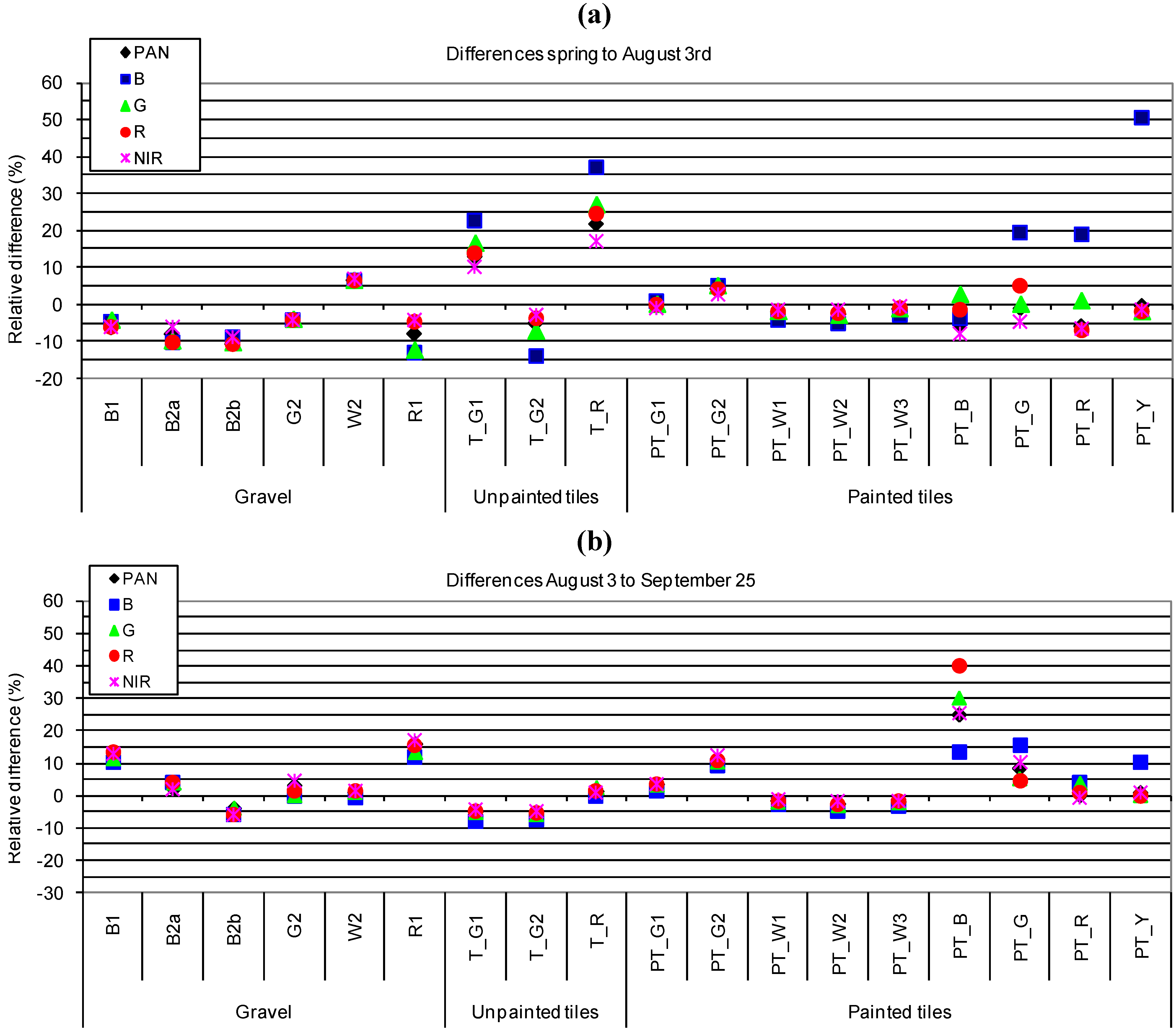
4.4. Temporal Stability

The spectra and anisotropy of the PAN channel in the principal plane, measured at different times, are shown in Figure 5, Figure 6 and Figure 7. We studied further the changes in the B, G, R, NIR and PAN channels at nadir (Figure 9) and the changes over the principal plane in the PAN channel (Figure 10) from May to June, from August to September and from May to September. The earlier measurement was used as reference in Equation 7; the negative values indicate darkening and positive values indicate brightening.

Figure 9. Changes in nadir reflectance of various objects in various channels from (a) May to August and (b) August to September. (Equation 7; the earlier measurement was used as the reference.)

Figure 9. Changes in nadir reflectance of various objects in various channels from (a) May to August and (b) August to September. (Equation 7; the earlier measurement was used as the reference.)

The changes on the different channels during the three-month period from May to August are shown in Figure 9a. The grey and black gravels and red gravel were getting darker and the white gravel was brightening. The changes were on the level of 5–10% for the grey, black and white gravels; for the red gravel the changes were different on different channels and rose up to 15%. For unpainted concrete tiles, the changes were larger at shorter wavelengths (the blue and green channel). One of the unpainted grey concrete tiles was darkening and another brightening during the period; the changes were up to 25% on the blue channel. The unpainted red tile got brighter during the period by 15–40%, depending on the wavelength. The changes to the painted grey and white concrete tiles were on the level of 5%; the white tiles were darkening and one of the grey tiles brightened slightly. For the painted color tiles, the changes were different on different channels; on the red, green and NIR channels the changes were −10% to 5% and on the blue channel up to 50% (the largest changes occurred on the yellow tile).

The changes during the two-month period from August to September are shown in Figure 9b. During this period, the gravels were brightening, excluding black gravel B2b. The changes were on the level of 5% or less on all gravels, excluding old black gravel B1 having differences of 10–15% and old red gravel R1, having differences of 10−20% depending on channel. For the unpainted concrete tiles, the changes were now quite similar in all channels; the grey tiles were darkening by 5–10% and the red tile did not change significantly. The white painted tiles darkened approximately 5% and the grey painted tiles brightened approximately 5% and 10%. For the painted color tiles, the changes were still different on different channels; the targets were brightening and the changes were 15–40% on the blue tile, 5–15% on the green tile, less than 5% on the red tile and 0–10% on the yellow tile.

The changes during the May-July and August-September periods occurred at a similar level and were slightly lower during the latter period. The changes were clearly lower during the August–September period on unpainted concrete tiles and on painted color tiles than in the spring period; a possible explanation for this difference is that the larger changes appeared on concrete when they were for the first time installed in outdoor conditions. In some targets, the changes to the same direction during the two periods indicated darkening and brightening processes. The darkening process appeared on the black gravel (B2b), one unpainted concrete tile (T_G2) and the painted white concrete tiles (PT_W1, PT_W2, PT_W3). The brightening process appeared on the painted grey concrete tiles. The reason for the darkening of the new gravel targets is probably the cleaning process, and the target with the largest change, new black gravel B2b, was probably the dustiest one at the beginning (Section 3.1). Regarding the painted concrete targets, the dark targets got brighter and bright targets got darker; this is known as the fading phenomenon, which occurs as the performance of the targets approaches the underlying concrete.

We studied the changes over the principal plane during all periods; as an example, the results from the May–September period on the PAN-channel are shown in Figure 10. For most targets, the variability in the differences over the observer zenith angles ±30° was relatively uniform, on the level of 5%, over the measurement period. A larger variability appeared on old black gravel (B1), grey gravel (G2), white gravel (W2), on one of the unpainted grey concrete targets, and on the painted grey concrete. For example, in Figure 10, the changes are uniform to a level of 5% over the observer zenith angles ±30° for all gravel targets, excluding grey gravel G2. The linear trend on the grey painted concrete tiles indicated that the targets brightened more in the backward direction than in the forward direction, which could mean that the targets might have lost their coarseness (Figure 10, right). The changes over observer directions of up to ±30° were mostly on the level of ±10% or lower. When we scaled the observations over the principal plane with the nadir observations, the differences were on the level of ±5% or less. Exceptions appeared on previously mentioned materials having larger than 5% variability in the differences over the principal plane. Larger differences appeared at the larger observer zenith angles, which occurred especially with gravel targets, partially due to differences in the illumination geometry (Section 4.3).

Figure 10. Differences of reflectance factors measured in spring and autumn at the principal plane on PAN channel (Equation 7, spring as reference). Left: gravel; center: concrete; and, right: painted concrete.

Figure 10. Differences of reflectance factors measured in spring and autumn at the principal plane on PAN channel (Equation 7, spring as reference). Left: gravel; center: concrete; and, right: painted concrete.

4.5. Influences of Moisture

The measurement results of the wet targets are given in Figure 5 and Figure 6. Moisture dramatically influenced the magnitude of reflectance, reflectance spectra and anisotropy.

The moisture caused a significant decrease of the magnitude of reflectance for all but the brightest targets: white gravel (W2), (Figure 5d), and white painted concrete tile (PT_W1), (Figure 6b). The ratio of dry to wet target was 2.7 for B2b, 2.6 for G2, 1.7 for R1, 1.1 for W2, 2.2 for T_G1 and 1.0 for PT_W1 on the PAN channel. For all targets, a significant drop of reflectance appeared in the water absorption bands at approximately 1400 nm and 1800 nm.

Moisture caused radical changes on anisotropy in the forward direction on all targets except the white gravel (Figure 5d). At the 60° forward observer zenith angle, the anisotropy was 10–40 times higher on wet targets than on dry targets; on white gravel the difference factor was two. At the 60° backward direction, the anisotropy factor decreased slightly, by a factor of 1.3 to 1.7. At the 10° observer zenith angle, the influences were not so serious; the anisotropy factor was less than 5% for all measured targets. Thus, at high observer zenith directions, the wet gravel targets were forward scatterers, excluding the white gravel; the forward scattering was highlighted on the wet concrete tiles.

5. Discussion and Recommendations

We presented the results of a comparative evaluation of various materials for permanent radiometric and colorimetric test sites of airborne imaging systems. The materials were new and old gravels and unpainted and painted concrete and they were characterized three times during 2009 in laboratory conditions using the FIGIFIGO goniospectrometer. We evaluated their reflectance spectra, reflectance anisotropy and stability as well as the influence of moisture.

5.1. Reflectance Properties

The black, grey and white gravel and the concrete and painted concrete materials provided a uniform reflectance spectrum, especially on visual and NIR channels. The average reflectances of the materials were 0.05, 0.10, 0.20, 0.30, 0.50 and 0.60. We also measured the color reference targets.

The anisotropy factors were typically on the level of 40–80% with observer zenith angles of ±60°, 10–30% with observer zenith angles of ±30°, and less than 5–10% with observer zenith angles of ±10°. This means that, if a 5% reflectance accuracy is required, the nadir spectrums could be used for observer zenith angles lower than ±10°; outside this region, the anisotropy has to be taken into account. We obtained these results with an illumination zenith angle of 45–60°, which is a typical illumination level in Finland in test-site calibration campaigns [2]. An analysis of gravel targets showed that, as the illumination elevation decreased, the anisotropy effects increased especially at large observer zenith angles. The results with gravels are consistent with our previous results [23].

5.2. Stability Aspects

We assessed temporal stability by carrying out measurements in spring, summer and autumn. New grey and black gravels were darkening, which was most likely due to the cleaning process of the new materials. Changes in the old black and red gravels were not systematic, indicating another phenomenon. For painted targets, the dark tiles were getting brighter and the bright tiles were getting darker; the reason for this could be that, as the paints wore out, the targets approached the properties of the unpainted concrete tiles. In the cases of concrete targets in particular, the different channels behaved differently. The results showed that for all types of targets changes greater than 5% are to be expected during the summer, but that, typically, changes of lower than 10% are achievable. Much larger changes appeared on the painted color targets.

Moisture caused dramatic changes on reflection properties. It decreased the magnitude of the reflectance spectrum significantly, in many cases more than 100%. Changes appeared in water absorption bands, and moisture also radically changed the anisotropy features.

If reflectance reference targets are kept in open-air conditions, significant changes in reflection properties will take place. Various phenomena can cause these changes. The cleaning process of gravel and the fading of concrete were already mentioned. Other anticipated factors include dirt on the surfaces (fine dust, pollen, etc.) and vegetation growing on the surface (for example, algae, moss, and lichen). Moisture and its interaction with materials (including biological materials) is expected to have the greatest influence [25,26]. All of these contribute in an interaction process causing seasonal, daily and cyclic changes, which are also dependent on weather conditions during the entire year [26]. In the optimum conditions, for example the Saharan deserts, the stability can be well below 5% [6, 21].

Durability and the performance of reflectance targets are dependent on local weather conditions (the amount of rain, sunlight, snow, frost, etc.) and, in general, on the environment (for example dust, pollutions, salinity, humidity), and the possibilities for cleaning and maintenance procedures. It is also possible to minimize the changes by covering targets when they are not used, but this requires a lot of maintenance efforts and is not considered to be a functional approach in Finland. Experience with gravel targets in Sjökulla has shown that white limestone in particular deteriorates over time and must be replaced occasionally, for example at 5–10 year intervals; black, grey and red granite targets keep their properties well and last for a long time, more than 10 years [12,23]. The experience with gravels is that dirt and dust are washed away naturally by rain, thus gravel does not require additional cleaning procedures. Concrete materials require cleaning during the imaging season in most cases. Unpainted concrete is durable but uncolored material does not provide a large reflectance range; positive experiences with red tiles indicate that colored concrete might be a potential approach. For painted concrete targets, re-painting is necessary, possibly every year. Of the evaluated materials, the painted and unpainted concrete tiles appeared to have better reflectance properties, especially in terms of isotropy, than the gravel targets. On the other hand, according to our experiences with challenging climatic and external conditions, the maintenance efforts of the gravel targets are lower than those of the concrete targets. Most of the evaluated targets were brought to field conditions at the beginning of the measurement period, and it is expected that different phenomena will appear with time. We will continue the monitoring process.

5.3. Recommendations

The conclusion in this study, related to the evaluated materials and the conditions, was that in situ measurements of reflectance targets were necessary for obtaining better than 5% accuracy. If calibration and validation were to extend outside the nadir region (±10°), the in situ measurement should be carried out from several directions. The optimal management of BRF should in the dynamic, open-air conditions, be further studied, for example the optimized measurement and modeling of BRF in stand-alone test sites.

Based on our recent results, we give the following recommendations for radiometric test sites of airborne systems (adopted from the CEOS requirements in Section 2.2, [6]):

• Sufficient spatial uniformity is required from the targets and the sizes of the targets should be at least 10 times the GSD. Targets should be located in flat and open areas. The characteristic of the surrounding surfaces should be further considered in order to minimize the influences of atmospheric adjacency effects.
• Targets with a large reflectance range, 0.03–0.90, are desirable, but, for example in photogrammetric applications and systems, a reflectance of 0.50 is often the upper limit, while from the point of view of atmospheric correction a reflectance of at least 0.30 is desired. Recent evaluations have shown that it is preferable to have several reflectance steps to characterize system radiometry over the entire dynamic rage (for example, 0.05, 0.20, 0.30, and 0.50) [28,29].
• A uniform spectrum is required for white and black targets, while for color and spectral targets different properties are of interest.
• Surfaces should be horizontal and they should have tolerable anisotropy. Surface reflectance should be accurately measurable for viewing angles up to ±60° to allow for calibrations of a wide range of photogrammetric and remote sensing systems.
• The stability of the targets should be tolerable against various external factors (for example, sunlight, rain, snow and dirt) and their construction and maintenance should be cost-efficient. The changes in targets are managed using appropriate measurement equipment.

We expect that accuracy of radiometric reference values could be improved to a much better level than 5%, which was aimed at this study, by improving the targets and measurement devices. More ideal targets could be sought by further fine-tuning the paint properties and surface roughness. Composing the surface by different materials might allow for some more optimization, for example when mosaicing black and white targets. The weather and moisture effects could be reduced by using water-repellent materials or heating to enhance drying or protection when not in use. Finally, it is important to realize that the requirements for the calibration and validation processes have to be based on requirements of applications and processes [22,30]; in the future more application-oriented studies are needed.

Analysis in laboratory conditions using a goniometer yields important controlled information on changes in materials, but is laborious when taking frequent measurements. Of interest would be to characterize the targets with an as-high-as-possible temporal resolution. Further analysis should be performed using airborne images collected over the targets. In outdoor conditions greater differences will be expected due to less stable measurement conditions and due to additional factors (especially humidity) influencing the reflectance [23,26]. One of the important topics for the future considerations is the assessment of the spatial uniformity of the materials.

6. Conclusions

We presented here a quantitative analysis of the suitability of various commercially available materials for permanent radiometric test sites. Analysis was performed especially from the point of view of multi-spectral photogrammetric sensors having a field of views of ±30°.

The targets varied significantly by their spectral and anisotropic properties. None of them met all the hoped for requirements, but all performed much better than just a randomly selected surface or paint. The brightest ones were the most isotropic, while the dark targets still pose a challenge. Gravel targets worked best from the nadir to the forward direction, while painted targets worked best from the nadir to the backward direction.

Achieving stability in the field is a challenge for every target. A target subject to weather is always subject to changes and requires regular cleaning and inspection. Wetness in particular caused large changes, and fast drying is one requirement for a field target. Otherwise excellent concrete targets took the longest time to dry.

The evaluated targets can provide a reference at an accuracy of 5–20%. When a higher accuracy is needed, real-time radiometric measurements must be performed. Efficient methods for in situ target reflectance and atmospheric measurements are crucial in addition to accurate targets.

The future challenge is the establishment of traceable reference reflectance values over a wide observation and illumination direction range under challenging climate conditions. This requires development of both materials and measurement equipment.

References

- Johnson, B.C.; Brown, S.W.; Rice, J.P. Metrology for remote sensing radiometry. In Post-Launch Calibration of Satellite Sensors; Morain, S.A., Budge, A.M., Eds.; Taylor & Francis: London, UK, 2004; pp. 7–16. [Google Scholar]
- Honkavaara, E. Calibrating Digital Photogrammetric Airborne Imaging Systems Using a Test Field. Ph.D. Dissertation, Helsinki University of Technology, Espoo, Finland, 2008. [Google Scholar]
- Pagnutti, M.; Holekamp, K.; Ryan, R.; Blonski, S.; Sellers, R.; Davis, B.; Zanoni, V. Measurement sets and sites commonly used for characterizations. In Proceedings of the ISPRS Commission I Symposium, Denver, CO, USA, 10–15 November 2002; In International Archives of Photogrammetry, Remote Sensing and Spatial Information Sciences. ISPRS: Vienna, Austria, 2002; Volume 34(1). [Google Scholar]
- Pagnutti, M.; Ryan, R.E.; Kelly, M.; Holekamp, K.; Zanoni, V.; Thome, K.; Schiller, S. Radiometric characterization of IKONOS multispectral imagery. Remote Sens. Environ. 2003, 88, 53–68. [Google Scholar] [CrossRef]
- Pagnutti, M.; Blonski, S.; Cramer, M.; Helder, D.; Holekamp, K.; Honkavaara, E.; Ryan, R. Targets, methods and sites for assessing the in-flight spatial resolution of EO data products. Can. J. Remote Sens 2010. (submitted). [Google Scholar] [CrossRef]
- Teillet, P.M.; Barsi, J.A.; Chander, G.; Thome, K.J. Prime candidate earth targets for the post-launch radiometric calibration of satellite sensors. In Proceedings of SPIE International Symposium, San Diego, CA, USA, August 2007; Volume 6677.
- Stensaas, G.L. US Geological survey digital aerial mapping camera certification and quality assurance plan for digital imagery. In Photogrammetric Week ’07; Fritsch, D., Ed.; Wichmann Verlag: Heidelberg, Germany, 2007; pp. 107–116. [Google Scholar]
- Cramer, M.; Grenzdörffer, G.; Honkavaara, E. In situ digital airborne camera validation and certification—The future standard? In ISPRS Proceedings of the 2010 Canadian Geomatics Conference and Symposium of Commission I, Calgary, AB, Canada, 15–18 June 2010.
- Chander, G.; Christopherson, J.B.; Stensaas, G.L.; Teillet, P.M. Online catalogue of world-wide test sites for the post-launch characterization and calibration of optical sensors. In Proceedings of IAC International Symposium, Hyderabad, India; 2007. [Google Scholar]
- Cramer, M. 10 Years ifp test site Vaihingen/Enz: An independent performance study. In Photogrammetric Week ’05; Fritsch, D., Ed.; Wichmann Verlag: Heidelberg, Germany, 2005; pp. 79–92. [Google Scholar]
- Casella, V.; Franzini, M. Experiences in GPS/IMU calibration. Rigorous and independent cross-validation of results. In Proceedings of ISPRS Hannover Workshop 2005, High-Resolution Earth Imaging for Geospatial Information, Hannover, Germany, 17–20 May 2005; p. 6.
- Honkavaara, E.; Peltoniemi, J.; Ahokas, E.; Kuittinen, R.; Hyyppä, J.; Jaakkola, J.; Kaartinen, H.; Markelin, L.; Nurminen, K.; Suomalainen, J. A permanent test field for digital photogrammetric systems. Photogramm. Eng. Remote Sensing 2008, 74, 95–106. [Google Scholar] [CrossRef]
- Iqubal, M. An Introduction to Solar Radiation; Academic Press: Waterloo, ON, Canada, 1983. [Google Scholar]
- Nicodemus, F.E.; Richmond, J.C.; Hsia, J.J.; Ginsberg, I.W.; Limperis, T. Geometrical Considerations and Nomenclature for Reflectance; U.S. National Bureau of Standards: Washington, DC, USA, 1977; p. 67. [Google Scholar]
- Schaepman-Strub, G.; Schaepman, M.E.; Painter, T.H.; Dangel, S.; Martonchik, J.V. Reflectance quantities in optical remote sensing—Definitions and case studies. Remote Sen. Environ. 2006, 103, 27–42. [Google Scholar] [CrossRef]
- Suomalainen, J.; Hakala, T.; Peltoniemi, J.; Puttonen, E. Polarised multiangular reflectance measurements using the finnish geodetic institute field goniospectrometer. Sensors 2009, 9, 3891–3907. [Google Scholar] [CrossRef] [PubMed]
- Schowengerdt, R.A. Remote Sensing, Models and Methods for Image Processing, 2nd ed.; Academic Press Inc: San Diego, CA, USA, 1997. [Google Scholar]
- CEOS Catalog of worldwide test sites for sensor characterization. Available online: http://calval.cr.usgs.gov/sites_catalog_map.php (assessed on 30 June 2010).
- Cosnefroy, H.; Leroy, M.; Briottet, X. Selection and characterization of Saharan and Arabian Desert sites for the calibration of optical satellite sensors. Remote Sens. Environ. 1996, 58, 101–114. [Google Scholar] [CrossRef]
- Loeb, N.G. In-flight calibration of NOAA AVHRR visible and near-IR bands over Greenland and Antarctica. Int. J. Remote Sens. 1997, 18, 477–490. [Google Scholar] [CrossRef]
- Smith, D.L.; Mutlow, C.T.; Rao, C.R.N. Calibration monitoring of the visible and near-infrared channels of the Along-Track Scanning Radiometer-2 by the use of stable terrestrial sites. Appl. Opt. 2002, 41, 515–523. [Google Scholar] [CrossRef] [PubMed]
- Honkavaara, E.; Arbiol, R.; Markelin, L.; Martinez, L.; Cramer, M.; Bovet, S.; Chandelier, L.; Ilves, R.; Klonus, S.; Marshall, P.; Scläpfer, D.; Tabor, M.; Thom, C.; Veje, N. Digital airborne photogrammetry—A new tool for quantitative remote sensing?—A state-of-the-art review on radiometric aspects of digital photogrammetric images. Remote Sens. 2009, 1, 577–605. [Google Scholar] [CrossRef]
- Peltoniemi, J.I.; Piiroinen, J.; Näränen, J.; Suomalainen, J.; Kuittinen, R.; Markelin, L.; Honkavaara, E. Bidirectional reflectance spectrometry of gravel at the Sjökulla test field. ISPRS J. Photogramm. Remote Sensing 2007, 6, 434–446. [Google Scholar] [CrossRef]
- Salamonowicz, P.H. USGS aerial resolution targets. Photogramm. Eng. Remote Sensing 1982, 48, 1469–1473. [Google Scholar]
- Wheeler, R.J.; LeCroy, S.R.; Whitlock, C.H.; Purgold, G.C.; Swanson, J.S. Surface characteristics for the alkali flats and dunes regions at white sands missile range. Remote Sens. Environ 1994, 48, 181–190. [Google Scholar] [CrossRef]
- Anderson, K.; Milton, E.J. On the temporal stability of ground calibration targets: implications for the reproductibility of remote sensing methodologies. Int. J. Remote Sens. 2006, 17, 3365–3374. [Google Scholar] [CrossRef]
- Kuittinen, R.; Ahokas, E.; Högholen, A.; Laaksonen, J. Test-field for aerial photography. Photogramm. J. Fin. 1994, 14, 53–62. [Google Scholar]
- Markelin, L.; Honkavaara, E.; Beisl, U.; Korpela, I. Validation of the radiometric processing chain of the Leica ADS40 airborne photogrammetric sensor. In ISPRS TC VII Symposium—100 Years ISPRS; Vienna, Austria, July 5–7, 2010, In International Archieve of Photogrammetry, Remote Sensing and Spatial Information Sciences; Wagner, W., Székely, B., Eds.; ISPRS: Vienna, Austria, 2010; Volume XXXVIII, Part 7A; pp. 145–150. [Google Scholar]
- Markelin, L.; Honkavaara, E.; Hakala, T.; Suomalainen, J.; Peltoniemi, J. Radiometric stability assessment of an airborne photogrammetric sensor in a test field. ISPRS J. Photogramm. Remote Sens. 2010. [Google Scholar] [CrossRef]
- Schaepman, M.E. Spectrodirectional remote sensing: From pixels to processes. Int. J. Appl. Earth Obs. Geoinf. 2007, 9, 204–223. [Google Scholar] [CrossRef] [Green Version]
© 2010 by the authors; licensee MDPI, Basel, Switzerland. This article is an Open Access article distributed under the terms and conditions of the Creative Commons Attribution license (http://creativecommons.org/licenses/by/3.0/).
Share and Cite
Honkavaara, E.; Hakala, T.; Peltoniemi, J.; Suomalainen, J.; Ahokas, E.; Markelin, L. Analysis of Properties of Reflectance Reference Targets for Permanent Radiometric Test Sites of High Resolution Airborne Imaging Systems. Remote Sens. 2010, 2, 1892-1917. https://doi.org/10.3390/rs2081892
Honkavaara E, Hakala T, Peltoniemi J, Suomalainen J, Ahokas E, Markelin L. Analysis of Properties of Reflectance Reference Targets for Permanent Radiometric Test Sites of High Resolution Airborne Imaging Systems. Remote Sensing. 2010; 2(8):1892-1917. https://doi.org/10.3390/rs2081892
Chicago/Turabian StyleHonkavaara, Eija, Teemu Hakala, Jouni Peltoniemi, Juha Suomalainen, Eero Ahokas, and Lauri Markelin. 2010. "Analysis of Properties of Reflectance Reference Targets for Permanent Radiometric Test Sites of High Resolution Airborne Imaging Systems" Remote Sensing 2, no. 8: 1892-1917. https://doi.org/10.3390/rs2081892