1. Introduction
The National Oceanographic and Atmospheric Administration (NOAA) and the National Aeronautics and Space Administration (NASA) have jointly developed a series of Polar Operational Environmental Satellites (POES). These Advanced TIROSN (ATN) spacecrafts are named after the prototype satellites, TIROS-N (Television Infrared Observation Satellites), which have flown since 1978 [
1]. The system consists of pairs of satellites, which ensure that every part of the Earth is regularly observed at least twice every 12 hours from about 800 km altitude. Starting with the NOAA-15 satellite in 1998, the satellites have an upgraded version of the Space Environment Monitor (SEM-2). The SEM-2 contains two sets of instruments that monitor the energetic charged particle environment near the Earth. These detect and monitor the flux of energetic ions and electrons in the atmosphere and the particle radiation environment at the altitude of the satellite.
The particle fluxes vary principally as a result of geomagnetic storms of solar origin, which depend on the temporal response of the magnetosphere plasma to the solar wind speed [
2]. Links between electron fluxes recorded by NOAA satellites and solar activity were studied in connection with geomagnetic storms [
3], under the radiation belts (L < 2) [
4] and in the inner belts (even with L < 2) within the South Atlantic Anomaly (SAA) [
5]. Similar studies have been carried out on NOAA proton fluxes in connection with geomagnetic storms [
6], under the radiation belts [
7] and inside them (L < 4) [
8]. These studies have shown the influence on the particle flux of the solar wind. In addition, the ionosphere is influenced by electromagnetic (EM) emissions of solar flares. Sudden Ionospheric Disturbances (SID) are caused by X-Ray and ultraviolet ionization and are followed by particle precipitation [
9]. SID are also produced by Gamma Ray Bursts as the X-Ray portion of these events will have the same effect as a solar flare X-Ray emissions [
10].
Trapped particles follow gyro- and bounce-motion between the hemispheres, as well as longitudinal drift, conserving the adiabatic invariant associated with the periodic motion [
11]. Longitudinal motion of trapped particles is dominated by the energy-dependent gradient-curvature drift [
12], in opposite directions for electrons and positively charged ions, rather than convection, which dominates the lower energy ring current [
13]. During quiet times, the trapped electrons are distributed into two belts divided by a slot at L = 2.5, around which there is relatively low energetic electron flux.
The SAMPEX satellite has provided a long-term global picture of the radiation belts [
14]. While the outer Van Allen Belt (VAB) (L > 2) varies with the solar cycle, semiannual and solar rotation time scales as well with geomagnetic storms, the inner VAB (L < 2) appears to have only solar cycle variations [
15]. The inner VAB is not in a stationary zone, but is affected by the influence of the magnetic activity, and magnetic storms can induce sudden electron flux enhancements of more than one order of magnitude near L = 2. A crucial point is to verify that contamination by very energetic particle fluxes and significant transport of electrons from the outer belt can be excluded. The NOAA satellite detectors allow an appropriate observation of particle dynamics and fluxes within a large L range and a comparison between the outer and inner VAB within the storm duration [
16].
Ionospheric disturbances linked to seismic activity were first observed around the time of the great Alaskan earthquake [
17] on March 28, 1964. Satellites measurements [
18] have confirmed the potential importance of this research, which provided medium and far field viewing points of lithosphere phenomena with respect to the earthquake (EQ) influence size. Estimations of the size of the EQ preparation zone, which is the same region where non-seismic phenomena have been observed [
19], range from 150 km for magnitude 5 EQs to more than 2,500 km for magnitude 8. A terrestrial observation of non-seismic phenomena linked to strong earthquakes should then produce local perturbations, which are strongly affected by several land and atmospheric variables, including anthropogenic disturbances. A satellite located at Low Earth Orbit (LEO), is at a distance from the Earth’s surface in the range of 200 km to 2,000 km, which is of the same order as the EQ preparation zone. Consequently, it is capable of observations enclosing the entire perturbed area [
20].
An interesting hypothesis based on the observation of Very Low Frequency (VLF) together with seismic activity [
18], suggested an EM link between particle fluxes and EQs, which was recently confirmed by the DEMETER satellite [
21,
22]. Experimental data of high-energy charged particle fluxes, obtained from various near-Earth space experiments (MIR orbital station, METEOR-3, GAMMA and SAMPEX satellites) were processed and analyzed; a 2 to 5 hour precursor effect was observed [
23], although the statistical significance was somewhat limited. A re-analysis of the SAMPEX database also showed a 4 hour precursor effect [
24]. Our analysis method followed the strategy introduced in 2005 for the analysis of SAMPEX data with some modifications [
25], since the NOAA satellites operate at higher orbits and cover different energy range intervals.
2. NOAA Particle Detector and Database Preparation
NOAA satellites contain particle detectors which monitor fluxes of protons and electrons at the altitude of the satellite. The satellites are placed in polar orbit (inclination angles of ~99°) at altitudes between 807 and 854 km [
1]. The particle detectors (Space Environment Monitor—SEM-2) consist of the Total Energy Detector (TED) and the Medium Energy Proton and Electron Detector (MEPED).
The MEPED is composed of eight solid-state detectors measuring proton and electron fluxes from 30 keV to 200 MeV [
26] which include the radiation belt populations, energetic solar particle events (protons) and the low energy portion of the galactic cosmic-ray population. The eight detectors consist of two proton telescopes which monitor the flux in five energy bands in the range 30 keV to 6.9 MeV, two electron telescopes which monitor the flux in three energy bands in the range 30 keV to 2.5 MeV, and four “omnidirectional” detectors sensitive to proton energies above 16 MeV. The opening angle aperture for the four directional telescopes is 30°. The geometric acceptances are ~0.1 cm
2sr. One telescope views at an angle of 9° with respect to the local zenith. The second telescope views in the orthogonal direction.
In comparison, the SAMPEX detector combinations provide low (1–4 MeV) and high (4–20 MeV) energy electron channels with a geometric acceptance of ~1.7 cm
2sr and an opening angle of the telescope of 58°. The elliptical orbit of SAMPLEX [
27] has an inclination angle of 82° with altitudes between 520 and 670 km and the configuration where a correlation appeared was equivalent to that telescope which views angle is 9°. Being so, NOAA detectors are both smaller and more directional than SAMPEX detectors.
The NOAA archive record [
26] represents a measurement period of 32 seconds of data, including a full set of orbital parameters provided every 8 seconds; in addition, satellite latitude and longitude are provided every 2 seconds. The archive record comprises 16 full data collection cycles from the MEPED electron and proton telescope instruments, so they are provided every 2 seconds with a sampling interval of 1 second. A selected portion of the SEM-2 instrument status, temperature, and system health data as well as data quality and ancillary information, are included. The first step in the preparation of NOAA data consists in the transformation of all binary files into Ntuples [
28]. Daily average geomagnetic and ionospheric activities were included in the Ntuples with the respective indexes Ap and SID to consider solar influence. Data were downloaded respectively from the National Geophysical Data Center (NGDC) at
ftp://ftp.ngdc.noaa.gov/STP/GEOMAGNETIC_DATA/APSTAR/apindex and from the American Association of Variable Star Observers (AAVSO) at
http://www.aavso.org/observing/programs/solar/sidbase/. Furthermore, we added the minimum L-shell mirror point altitudes obtained with the UNILIB libraries [
29] to determine if particles were precipitating.
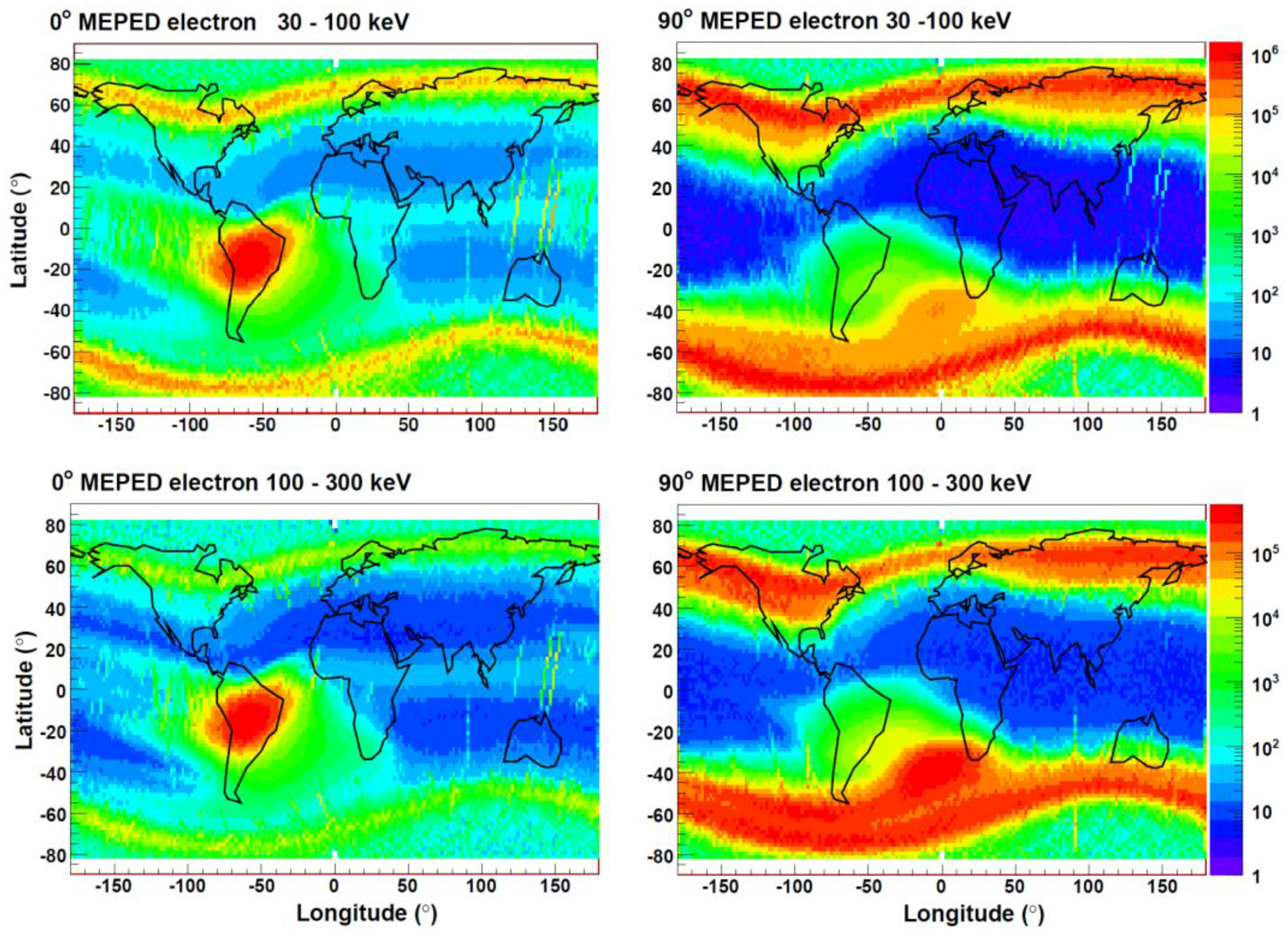
As all sets of orbital parameters are provided every 8 seconds, we chose this value as the basic time step for our study. Consequently, all other variables were defined with respect to the 8 second step. Thus, 8 second averages of counting rate (CR), latitude, longitude, MEPED and omnidirectional data were calculated. Unreliable counting rates with negative values were labeled and excluded from the analysis. Since the energy detected for the electrons is a cumulative sum over three thresholds equal to E1 = 30 keV, E2 = 100 keV and E3 = 300 keV, we defined new energy channels derived from the difference of the energies thresholds to obtain electrons detected in the intervals 30–100 keV, 100–300 keV and >300 keV, which are similar to the proton energies channels and are shown in
Figure 1. Unreliable CRs were defined and excluded when E2 − E1 < 0 and when E3 − E2 < 0.
Figure 1.
The average electron flux (cm2s−1sr−1MeV−1) in geographical coordinates. Channels are defined in orientation directed towards the zenith (0°) and perpendicular to the direction of the satellite motion and zenith, in energy with respect to the bands 30–100 keV and 100–300 keV. The scale on the right indicates the average annual (2003) electron flux. The red spot of the 0° electrons (left) represents the SAA where the satellite go through the inner VAB (L < 2) and so the detected electrons are trapped particles. Similarly, near the poles, trapped particles are also visible with the lobes in the 90° electrons (right), differences in shape was given from the pitch angle selection.
To correlate seismic activity with NOAA data we created a Ntuple, which contains EQs data including: event time, location, magnitude and depth. These data were downloaded from the Earthquake Center of United States Geological Survey (USGS) at
http://neic.usgs.gov/neis/epic/epic.html. The values of the corresponding L-shells of the EQ epicenter projected to different altitudes were also calculated by UNILIB and included in the Ntuples. This was done to determine the presence and location of a possible link between EQ and particle fluxes and will be explained in
Section 4.
3. NOAA Data Analysis
We calculated the daily averages of CRs and then defined the condition for which a CR fluctuation was not likely due to possible statistical fluctuations with a probability larger than 99%, the particle burst (PB). According to previous work [
23,
24,
25], the daily averages of CRs were calculated in the invariant coordinates space. This choice was very useful to obtain more stable results, as particle motion is strongly variable along the satellite orbit. Together with the L-shell and the pitch angle α, it was necessary to take into account the CR amplitudes and variation
versus geomagnetic coordinates, since the spatial gradient of particle fluxes near the SAA is too large. The geomagnetic field magnitude B can be considered a suitable parameter for delimiting the transition region between inner and outer radiation belts [
30] where large gradients are located and sub intervals of the B are defined, so to limit the CR amplitude variations. Nonetheless, some regions remain where the particle fluxes and their variations were very high, when the satellite went through the VAB in the polar regions and in the SAA. In this analysis, the SAA was excluded by choosing B > 20.5 μṬ; and external VAB were excluded by choosing L < 2.2.
Then the averages were calculated in every sector of a three–dimensional matrix formed by the shell, pitch angle and geomagnetic field intervals. The L-shell bin’s width was set to 0.1 as in the past analysis [
24] and the range chosen between 0.9 and 2.2. In this study, the pitch angle is equal to the difference between the particle telescope and geomagnetic field directions. The SEM-2 detectors, however, have a finite aperture of 30°, thus we chose a bin width of 15°. The geomagnetic bin width was fixed to be dependent on shorter intervals going through the radiation belts, because we need to compensate for the non–linear increases in CR when the satellite goes near the SAA. The following six B bins were used to calculate averages: 20.5–22.0 μΤ, 22.0–25.0 μΤ, 25.0–29.0 μΤ, 29.0–33.0 μΤ, 33.0–37.0 μΤ and 37.0–41.0 μΤ. To obtain a reliable statistic, we demanded that the satellite passed at least 20 times a day through the same cell.
In
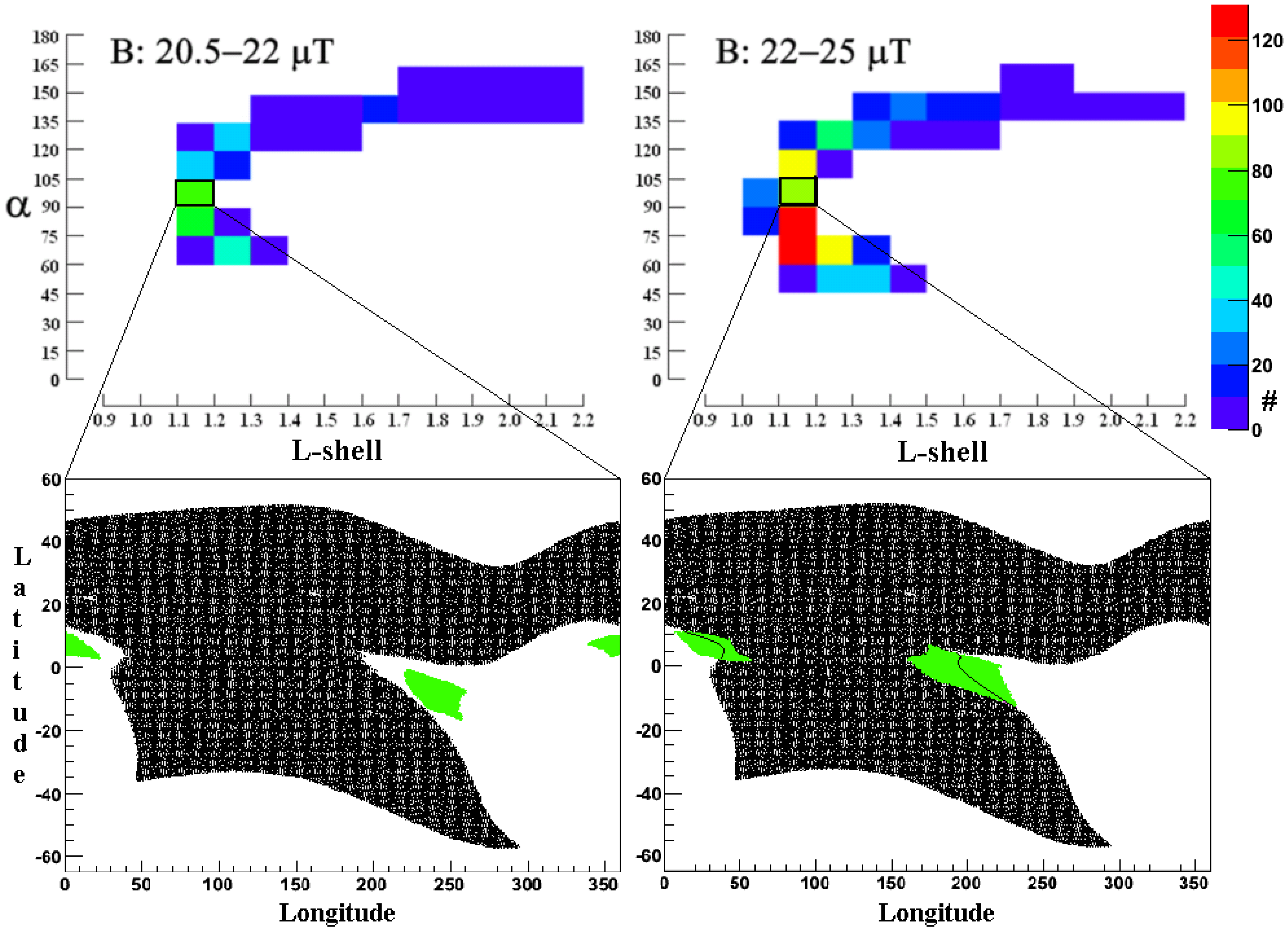
Figure 2 the satellite positions used in the analysis with the corresponding bin occupation in (L, α, B) are shown. The black area indicates the satellite locations corresponding to observed particle precipitation, the green area shows the satellite geographical positions corresponding to the cells where B = 20.5–22.0 μT and B = 22.0–25.0 μΤ, with 1.1 < L < 1.2 and 90° < α < 105°. Only CRs in the intersections between black and green areas were considered to study perturbations to VAB as they are precipitating particles that will be released from the trapping. CR distributions inside such areas are compatible with a Poisson distribution in agreement with earlier works [
24]. We introduced a threshold in sigma [
25] so that the amplitude of the CRs must exceed the average value to define the conditions for which a CR is a non-poissonian fluctuation with 99% probability as shown in
Figure 3.
Figure 2.
Top, the data distribution in L, α for two selected B-field values. Bottom, the data distribution in latitude and longitude, and for the two selected (L, α, B) bins (green), and the precipitating particle distribution (black).
Figure 2.
Top, the data distribution in L, α for two selected B-field values. Bottom, the data distribution in latitude and longitude, and for the two selected (L, α, B) bins (green), and the precipitating particle distribution (black).
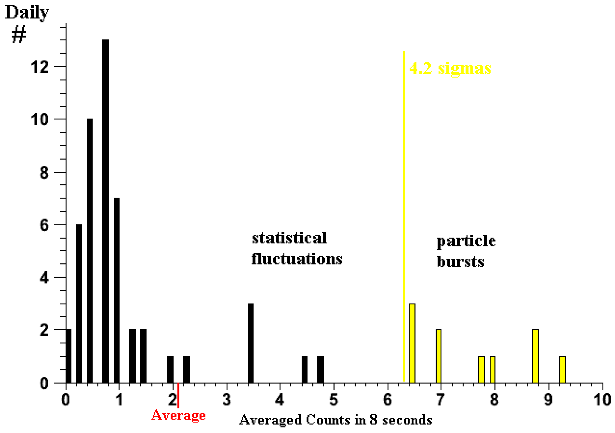
Figure 3.
CR distribution in the green cell of
Figure 2, where 1.1 < L < 1.2, 90° < α < 105° and 22.0 μΤ < B < 25.0 μΤ. As the CR was the average of 4 CRs in 8 seconds, the fractional values and significance must be redefined [
25]. To have <1% probability to be a poissonian fluctuation, CRs must exceed the 4.2 sigmas threshold.
Contiguous PBs were defined from 8 second PBs by simply joining a continuous set of PBs, up to a maximum duration of 600 seconds [
31]. Because VAB are densely populated and strongly influenced by solar activity, we were interested in anomalous particle fluxes outside VAB, detected during solar quiet days. The NOAA satellites go through the VAB in the SAA and polar regions, thus these regions can be excluded by selecting respectively a minimum L-shell mirror point altitudes ≤ 100 km and L ≤ 2.2. SAA region corresponds to the white area at medium and low latitudes of
Figure 2, within this area particles are trapped at NOAA satellite altitudes, CR increase quickly and we are not able to extract information about the weak disturbances of the VAB.
Particle precipitation from the lower boundary of the radiation belts can be described as a result of pitch angle diffusion and drift around the Earth along an L-shell [
32]. Along the drift, the altitude of the mirror points varies and when the particles fall below 100 km they interact with the atmosphere and are lost. With the UNILIB software we calculated the minimum L-shell bouncing altitudes H
mirror, so we could select particle precipitation events by the condition H
mirror ≤ 100 km. An example of selected PBs from the NOAA-15 database is shown in
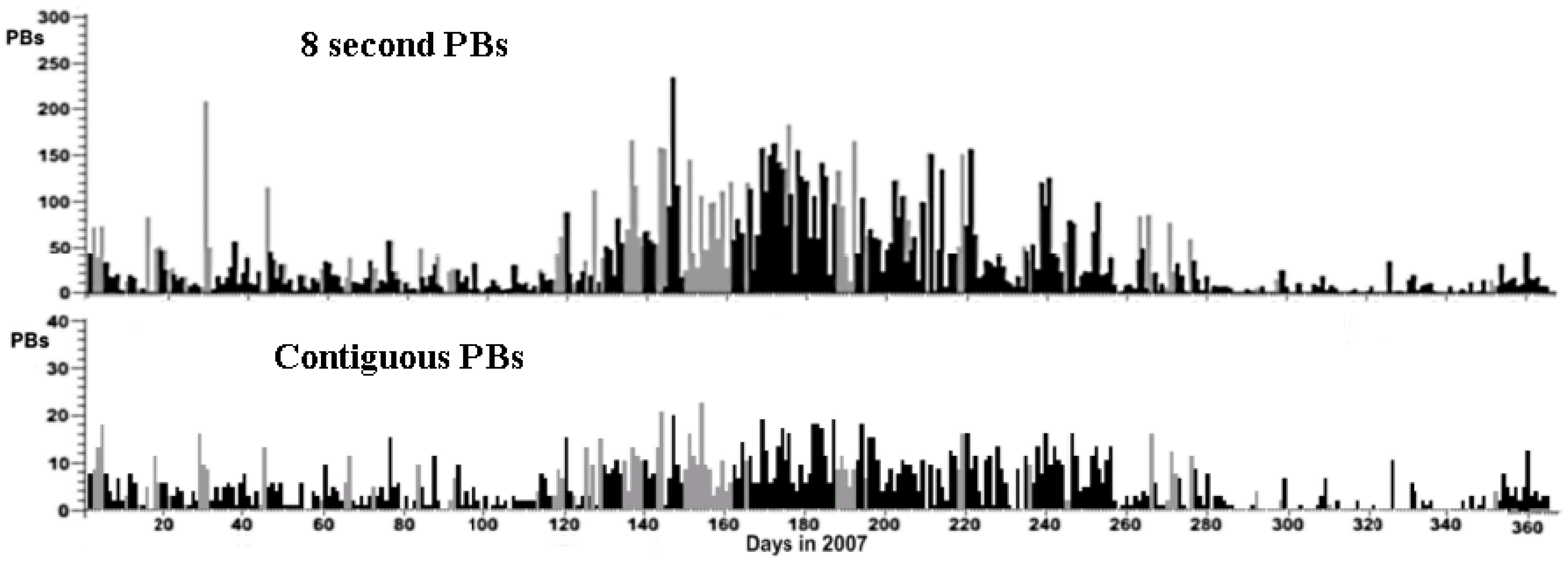
Figure 4 for the year 2007, 8 second and contiguous precipitating PBs are represented in black to identify quiet solar periods (Ap ≤ 15 and SID = 0) and in gray for the solar perturbed periods (Ap > 15 and SID = 1), as we stated in a previous work [
25]. A summary of the electron contiguous PB activity during 11 years of NOAA-15 database was shown for the 0° detector, with electron energy from 30 keV to 100 keV [
31].
Figure 4.
The daily distribution of elementary (8 second) and contiguous PBs during solar quiet (black) and solar perturbed (gray) periods in 2007 of the NOAA-15 electron detector at 0°, in the energy range 30–100 keV.
Figure 4.
The daily distribution of elementary (8 second) and contiguous PBs during solar quiet (black) and solar perturbed (gray) periods in 2007 of the NOAA-15 electron detector at 0°, in the energy range 30–100 keV.
4. Correlations between Particle Bursts and Earthquakes
To calculate the correlation we followed the methods used in the past [
23,
24]. We supposed that the possibility of EM wave-particle interaction may have taken place within the lower boundary altitude of the inner radiation belt, ranging between 200 km and 2,400 km. We used the L-shell value LEQ corresponding to the EQ projection epicenter as a parameter, which defines the altitude influence of seismic activity, considering in this case only strong EQs with magnitudes M ≥ 5. Given that the VAB is a system in which regions with the same L-shells behave in the same way when responding to external stimuli, we calculated the L
PB values of the detected PBs at the satellite altitude and compared them with the corresponding L
EQ values of EQs, see
Figure 5. This was possible because precipitating particles drift longitudinally around the Earth along a fixed L-shell, eastwards for electrons, and the L-shell is not modified after the EM wave-particle interaction. The EQs and PBs L-shells were calculated through UNILIB by using EQ epicenters and satellite co-ordinates.
Now we considered the subsets of EQs and PBs which meets the condition
which plays the role of simulating the physical interaction, whatever it is, and was imposed to select PBs and EQs. The meaning of (1) puts in relationship EQs and all PBs whose particles passed at a well defined altitude above the EQ epicenters, even if the satellite detects them at different latitudes, longitudes and altitudes. In other words, every EQ is considered in connection to all the precipitating particles which belong at the same shell of the VAB, this shell has a precise altitude above the EQ epicenter. This implies that an indirect or mediated action perturbs the particle motion, consistent with an EM disturbance [
24].
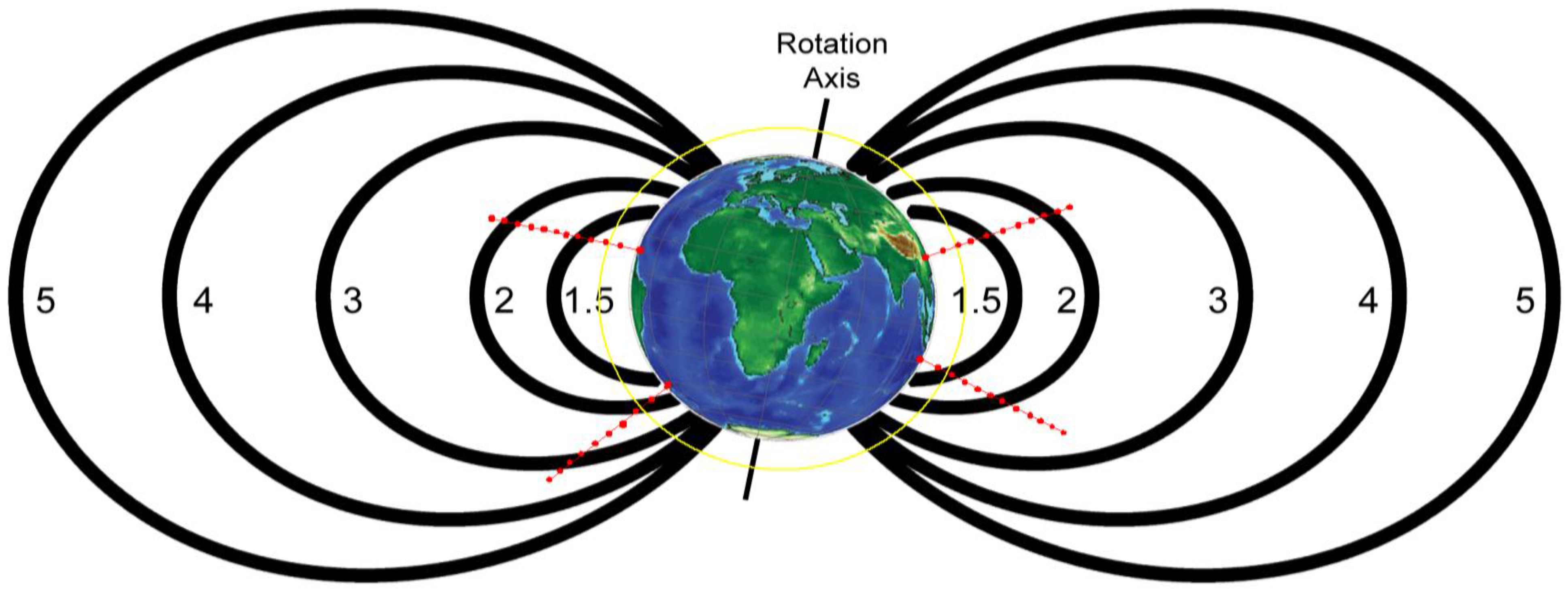
Figure 5.
A sketch representing the satellite orbit (yellow) and earthquake epicenter projections (red) with respect to the L-shells. We can see that the satellite passes through high L-shells at the poles, while EQ epicenters projections cover only low L-shell values as the EQ epicenters at high latitudes are rare.
The time differences T
EQ − T
PB between seismic and particle precipitation events collected in the Ntuples, which satisfied the L-shell conditions defined above for different EQ altitude projections, are in the ranges |T
EQ − T
PB| ≤ 3, 30 and 150 days in filling the correlation histograms. The complete 11 year NOAA-15 database, from the beginning of July 1998 to the end of June 2009, was processed and correlated to the same period EQ events, and the histogram distributions were generated for several cases. Use of the Root facilities [
33] permitted any Ntuple variables to be used as an additional parameter; for example, by further selection on the magnitude of the EQs and the L-shell differences. Given that the PB selection algorithm was limited to regions with low particle fluxes, the resulting EQ positions to be taken in account were restricted to ±25° from the equator. Thus, the analysis principally concerned EQs of Indonesian and Peruvian regions where typically EQs are stronger.
Correspondingly, the L-shell limits restricted the analysis to the inner VAB. Furthermore, the selected PBs occupied primarily the positions west of the excluded SAA region, and near the equator. Since the inner VAB mirror points cross the trajectory of the satellite, consequently electrons drifting eastward are detected by the NOAA instruments before they precipitate in the SAA. If the longitude of PB detections and EQ epicenters are different, their physical link remains since electrons moving eastward along the same L-shell allow the perturbed particles over the EQ epicenters to be detected when their pitch angle and the detector orientation are compatible, see
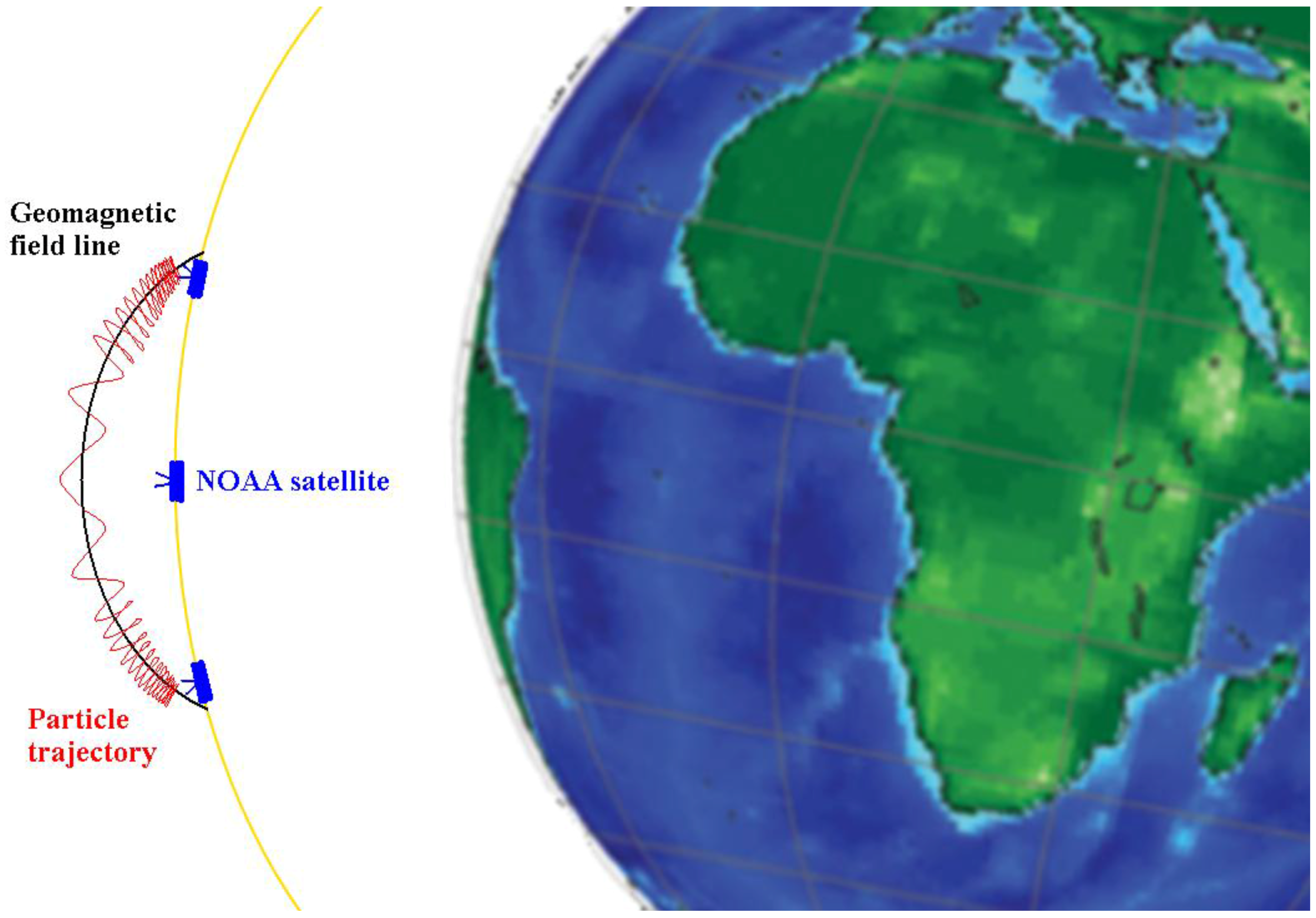
Figure 6.
Figure 6.
In the region just west of the SAA, the satellite orbit (yellow) crosses the mirror points of the geomagnetic line (black) of the internal VAB. In this region, the particle trajectories (red) can be detected by the 0° detector which has an aperture of 30°. At different longitudes the orbit crosses the same shell at different points.
We initially evaluated the fluctuations obtained from both the 8 second and contiguous PBs of
Figure 4. The results between the two definitions were very different as the 8 second PB distributions produced very large correlation fluctuations and this led us to discard the former PB definition. The continuous PB definition was acceptable as the fluctuations were compatible with the Poisson processes. However, this was true only within well defined parameter ranges, while in general fluctuations were greater due to the sensibility of the NOAA satellites to solar activity [
34]. To exclude effects due to solar activity, we used the Ap index value equal to 15 [
25,
31]. We describe the cases where significant correlations appear.
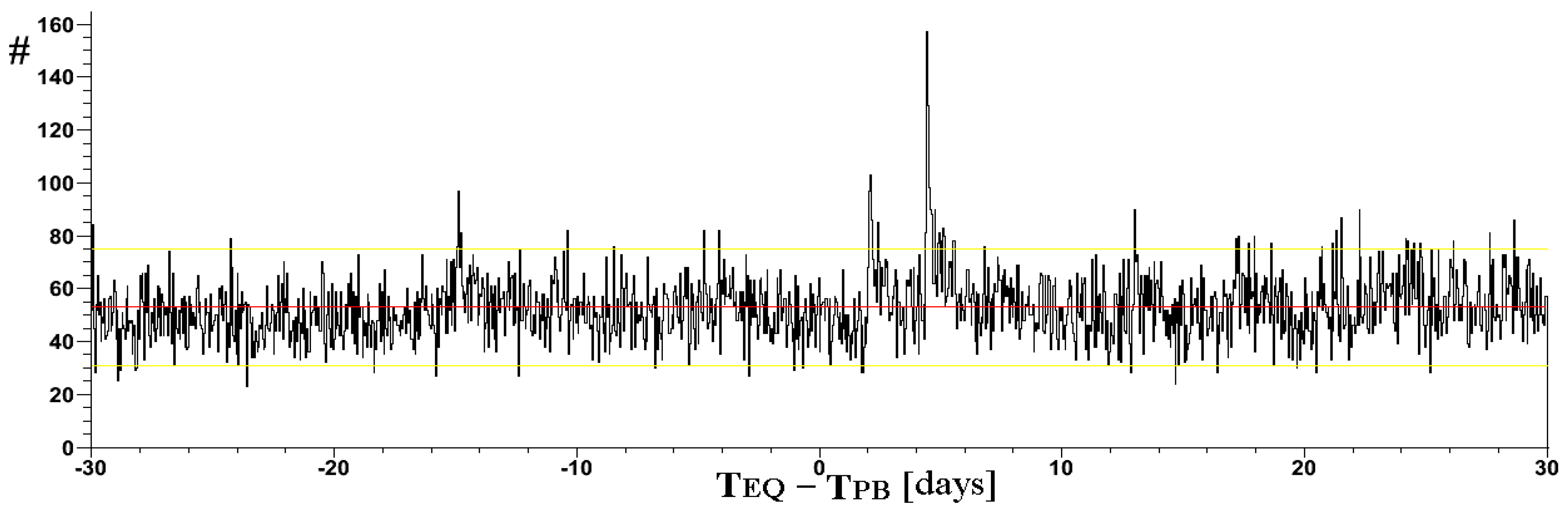
The first case occurred between EQs of magnitude M ≥ 5 for altitudes greater than 1,000 km in the 0° electron energy range of 100–300 keV (
Figure 7). The correlation is found 4.4 days before EQs. It appeared over several low altitude EQ projections and the 1,400 km projection altitude of the EQ epicenters was the most significant for all projections. This fluctuation was more than 12 sigmas above the average (red) and the distribution was not flat; in
Figure 7, the three sigma significance (yellow) for a Poisson process is also indicated. Also, the channel of 0° electrons in the energy range of 30–100 keV correlated positively with the same EQs: 6 day after and 10.6 day prior to, with respect to the EQs for 400–600 km EQ epicenter projections, and more complicated structures for higher altitudes.
Figure 7.
Correlation time within 30 days of global EQ activity and NOAA 15 PBs. EQs and PBs were selected from an 11 year database, from July 1998 to July 2009, with the condition |LEQ − LPB| < 0.1. In this plot, EQ epicenters were projected at 1,400 km and mirror altitudes PBs were less than 100 km. The red line shows the average and the yellow lines show the 3 sigmas significance. Binning was 1 hour.
It was revealed that the 4.4 day peak was principally produced by the Sumatra seismic events in December 26, 2004, which consisted in several strong EQs in a small time window or, in other words, an EQ cluster. Other correlations were shown to be linked to the same Sumatra and other big EQ clustering. The 4.4 day correlation can be explained as a combination of clustering and selection rules. In fact, every EQ is characterized by a longitude and, due to the asymmetry of the geomagnetic field, different longitudes select different L-shells at same altitude projection. So, clustering of EQs define many EQs with the same L-shell for the same altitude projection in a small time interval while few EQs of M ≥ 5 in a day are usually characterized by different L-shells. The link with PBs is established by their nearer L-shell, which is very infrequent and usually performed with only one EQ, for this reason the correlation with a cluster is an exceptional case.
To remove the clusters from the EQ database we used the program CLUSTER 2000 [
35]. It was downloaded from
ftp://ehzftp.wr.usgs.gov/cluster2000/cluster2000x.f and updated as to include years after 2000, in this way we are able to label the aftershock events and discard them. We used this software with the variation of unique parameter that was the number of crack radii [
36], it was fixed initially equal to 10.
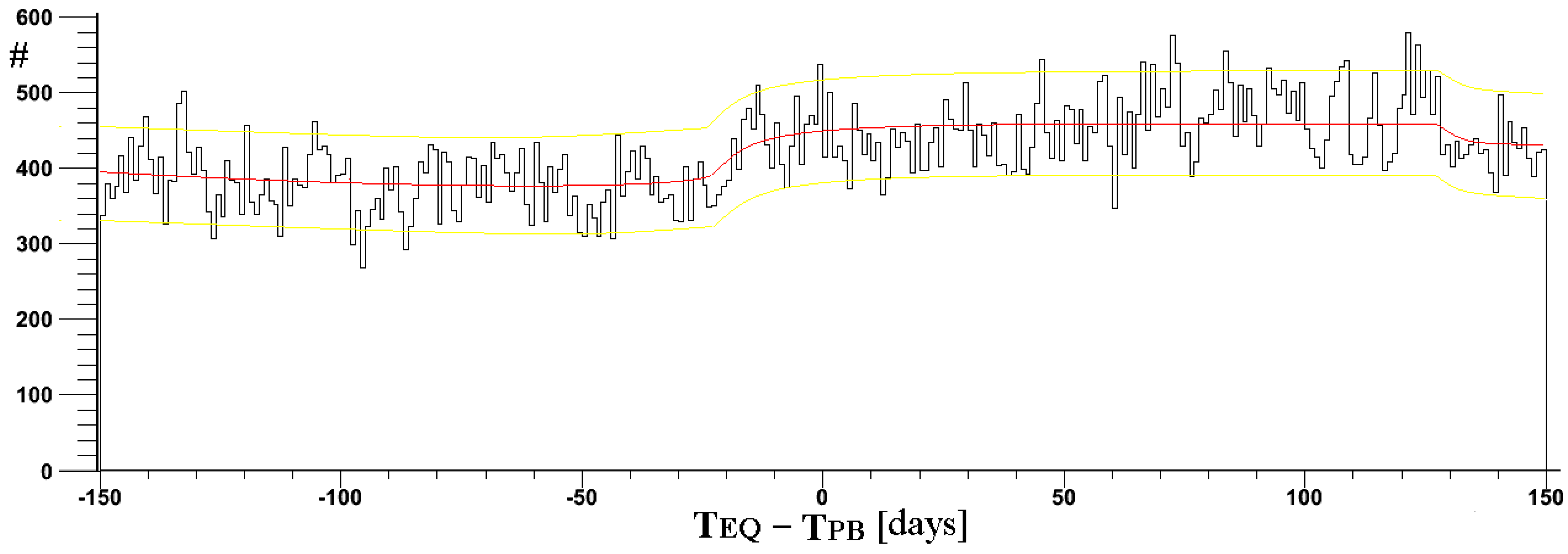
Figure 8.
If PB electrons in the energy range of 30–100 keV were compared with M ≥ 6.2 EQ epicenters projected to 800 km, a step correlation appears which has a seasonal time length. The red line represents the average while the yellow lines represent ±3 sigmas from the average. Distributions binning was of one day.
Another less evident, but relevant correlation appeared between EQs and PBs when analyzing larger time intervals. A step in the correlation distribution was noted around −20 days for electron PBs in the energy range of 30–100 keV when projecting EQ epicenters at 800 km. The greater correlation with increasing time difference remained for a long period from −20 up to 130 days, it is more evident for magnitude M ≥ 6.2 EQs (shown in
Figure 8) where the time difference between the EQs and PBs was 150 days. It can be described as a step in the correlation which increased the correlation average for several months; the increase appeared to have a seasonal period. This correlation was evident for EQ epicenters altitude projections between 200 and 1,400 km. The EQ and PB frequency comparison showed an association between a group of large EQs and the boreal summer increase of PBs. In this case, a small increase in global high seismic activity correlated with summer increase of PBs, shown in
Figure 4. The binning of the correlation was chosen to be one day to enhance the effect, but similar results are obtained with binning of one hour; the correlation at 4.4 days also appears with the binning of one day.
The correlations in
Figure 8 revealed some strong seismic events which were still clustered. Such aftershocks concerned big EQs where fault lengths were very much greater than their depths. Therefore, they were completely removed by increasing the number of crack radii up to 1,000. The new EQ database was used to calculate the EQ-PB correlation distributions which were finally free from these influences and ready for further analysis. To take in account the summer increase of the PBs, and considering that the daily number of PBs is very high in the summer (
Figure 4), a new definition of correlation was given, in which PBs are harmonically modulated between 1/2 and 1/3 from May to September. The weight function was chosen to be
where Dy is the day of year and D is the total number of days in the year. It was equivalent to calculate a weight correlation where the weight was less than 1 for the summer months.
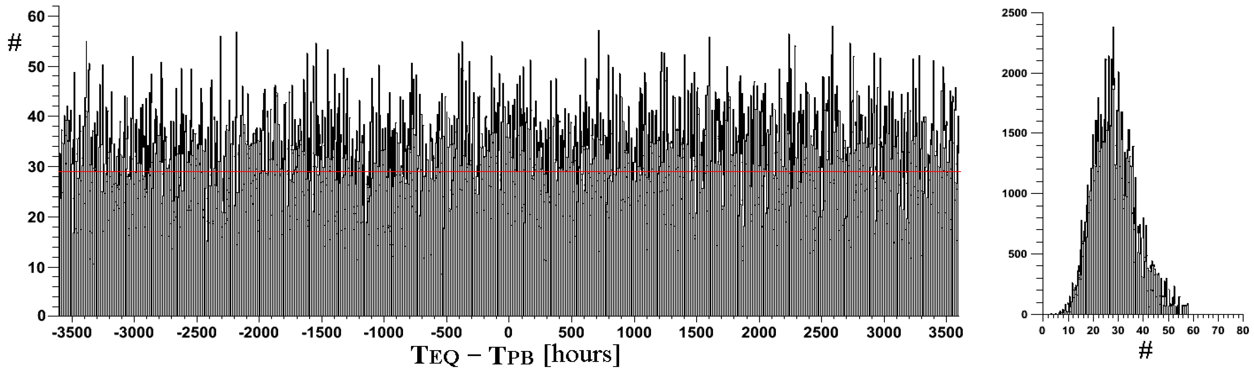
Through this new definition, the step in the distribution disappeared and a flat correlation was obtained for all the altitude EQ epicenter projections compared with the lower energy channel of electron data, in
Figure 9 the example of 800 km EQ altitude projections is given. The binning of this correlation was one hour. The average correlation was 28.19 and sigma was 7.97, so that we have sigma greater than root square of the average. The same ratio between sigma and average was also verified for the correlations calculated by all the others EQ altitude projections. Correlation distributions were compatible with a super-poissonian distribution which fit in a better way the fluctuation distribution on the right of
Figure 9. In all studied cases of correlations of different EQ altitude projections, no significant correlation appeared for EQ magnitude M ≥ 5 at this stage of the analysis.
Figure 9.
Correlation between M ≥ 6 EQs and continuous PBs where EQ epicenters were projection to 800 km and time differences was considered up to 150 days (left). The binning in this case was one hour. The red line is the average. The fluctuation distribution is shown on the right, it is a super-poissonian distribution.
