1. Introduction
Remote sensing applications for natural resources using unmanned aircraft systems (UAS) as the observing platform have grown considerably in recent years. This increase has been observed not only in practical applications, but also in the peer-reviewed literature. Two recent special issues on UAS for environmental remote sensing applications in the journals Geocarto International [
1] and GIScience and Remote Sensing [
2] as well as other recent publications reflect the growing acceptance by the remote sensing community of UAS as suitable platforms for acquiring quality imagery and other data for various application such as wildfire mapping [
3,
4], arctic sea ice and atmospheric studies [
5], detection of invasive species [
6], rangeland mapping [
7,
8,
9], hydrology and riparian applications [
10,
11,
12], and precision agriculture [
13,
14,
15,
16]. Due to limited payload capacities on small unmanned aerial vehicles (<50 kg), consumer digital cameras are often used. Such configurations have been employed successfully for mapping Mediterranean forests [
11], arid rangelands [
17,
18], aquatic weeds [
19], soils [
20], and crops [
13]. Using texture and/or the intensity-hue-saturation components can compensate for the low radiometric and spectral resolution of consumer cameras [
9,
21], although the lack of a near infrared band poses certain limitations for vegetation characterization. Quality lightweight multispectral sensors suitable for use on small UAS have not been widely available in the past, and one alternative has been to alter consumer cameras to acquire images in the near infrared band [
14,
22,
23]. A multispectral sensor that captures data over a range of relatively narrow wavelength bands is preferable for vegetation applications because of the potential for quantitative remote sensing, retrieval of biophysical parameters, better differentiation of vegetation species, and greater suitability for comparison with satellite imagery. Despite the potential of UAS to acquire high spatial resolution multispectral data, research in this area is relatively limited, and only a few applications have been reported in the literature.
Huang
et al. [
24] used a compact multispectral camera (ADC, Tetracam Inc.) to acquire data in the red, green, and near infrared bands for agricultural applications. The authors listed as pros the low cost and light weight of the camera, but reported that slow imaging speed, band saturation, and low image quality limited its applications and potential for true radiometric correction of the data. The same camera was used on an unmanned helicopter by other researchers, who reported more favorable results, including high correlations for field and image-based estimates for rice crop yield and biomass [
25].
A higher quality multispectral sensor (MCA-6, Tetracam, Inc.) was used for retrieving various biophysical parameters and detecting water stress in orchard crops and the researchers concluded that quantitative multispectral remote sensing could be conducted with small UAS, although the area covered was limited by the endurance of the UAS [
15,
16]. Turner and Lucieer [
26] presented promising preliminary results using imagery acquired from an unmanned helicopter equipped with visible, thermal, and multispectral sensors for precision viticulture applications. While individual image acquisition costs vary depending on the platform, required personnel, and legal restrictions [
27], it is generally agreed that, compared to piloted aircraft, the major advantage of a UAS-based approach is the ability to deploy the UAS repeatedly to acquire high temporal resolution data at very high spatial resolution.
A UAS-based image acquisition commonly results in hundreds of very high resolution (cm to dm pixel size), small footprint images that require geometric and radiometric corrections and subsequent mosaicking for use in a Geographic Information System (GIS) and extraction of meaningful data. An efficient workflow is necessary for the entire processing chain so that end products of a given accuracy can be obtained in a reasonable time. The position and attitude data acquired from UAS often suffer from lower accuracy compared to data acquired with piloted aircraft, and various custom approaches have been developed for orthorectification and mosaicking of UAS imagery [
28,
29,
30,
31]. Radiometric correction can also be challenging due to the (potentially) large number of individual images, image quality, and limits over the control of image acquisition parameters [
24]. Obtaining radiometric ground measurements for calibration can be time consuming and costly, even with piloted aerial image acquisitions [
32]. Empirical line calibration methods have been used for radiometric normalization of multispectral UAS imagery to obtain quantitative results for various crop applications [
16,
33,
34], but no multispectral UAS applications have been reported for rangelands.
This study builds on previous work on development of workflows for UAS-based image acquisition, processing, and rangeland vegetation characterization using low-cost digital cameras [
8,
17,
18]. The goal of this study was to develop a relatively automated and efficient image processing workflow for deriving geometrically and radiometrically corrected multispectral imagery from a UAS for the purpose of species-level rangeland vegetation mapping. The methods for orthorectification and mosaicking of the multispectral imagery follow closely the approaches we developed for low-cost digital cameras [
8,
29]. The main focus of this paper are the description of challenges and solutions associated with efficient processing of hundreds of multispectral UAS images into an orthorectified, radiometrically calibrated image mosaic for further analysis. We detail the batch processing methods, compare two approaches for radiometric calibration and report on the accuracy of a species-level vegetation classification for a 100 ha area. In addition, we provide a comparison of spectral data obtained from UAS imagery and a WorldView-2 satellite image for selected vegetation and soil classes. There is great potential for upscaling high resolution multispectral UAS data to larger areas, and the WorldView-2 imagery with its relatively high resolution and eight bands is well suited for this purpose.
2. Methods
2.1. UAS, Sensors and Image Acquisition
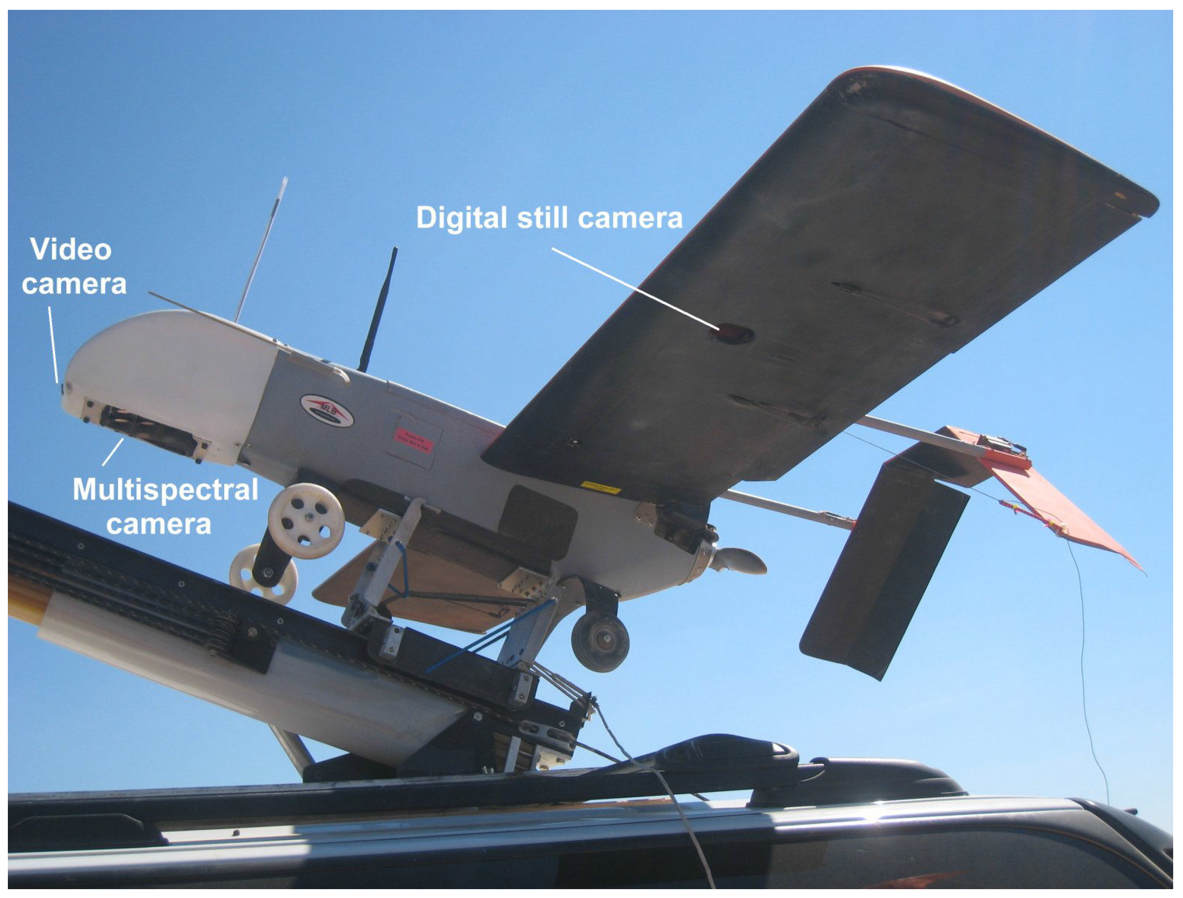
We used a BAT 3 UAS (MLB Co., Mountain View, CA, USA) for aerial image acquisition (
Figure 1). The BAT 3 weighs 10 kg, has a wingspan of 1.8 m, and is catapult launched from the roof of a vehicle. The BAT 3 has an endurance of up to six hours, but the camera’s data storage capacity usually limits flights to approximately two hours.
The aircraft is equipped with three sensors: a forward looking color video camera, used for live video downlink, and two cameras, a Canon SD 900 ten megapixel compact digital camera in the wing, and a Mini MCA-6 (Tetracam, Inc., Chatsworth, CA, USA) in the modified nose of the aircraft. Both still cameras acquire imagery simultaneously with a 75% forward lap and 40% side lap for photogrammetric processing. The image acquisition, processing, and analysis based on the Canon SD 900 imagery has been reported previously [
8,
9,
18]. In this paper, we are focusing on the processing and analysis of the multispectral images acquired with the Mini MCA-6 (MCA hereafter (for multi-camera array)).
Figure 1.
BAT 3 unmanned aircraft systems (UAS) positioned on the catapult on the roof of the launch vehicle. The UAS is equipped with a small video camera, a Canon SD 900 digital camera in the wing, and a Mini MCA multispectral camera in the nose.
Figure 1.
BAT 3 unmanned aircraft systems (UAS) positioned on the catapult on the roof of the launch vehicle. The UAS is equipped with a small video camera, a Canon SD 900 digital camera in the wing, and a Mini MCA multispectral camera in the nose.
The MCA is a light-weight (700 g) multispectral sensor (cost of US $ 15,000) designed for use on a small UAS. Six individual digital cameras with lenses with a focal lens of 8.5 mm and a 1.3 megapixel (1,280 × 1,024 pixels) CMOS sensor are arranged in a 2 × 3 array. Images can be acquired with 8-bit or 10-bit radiometric resolution and are stored on six compact flash (CF) cards. The cameras have interchangeable band pass filters (Andover Corp., Salem, NH, USA), and for this study, we used filters with center wavelengths (band widths at Full Width Half Maximum in brackets) at 450 (40), 550 (40), 650 (40), 720 (20), 750 (100), and 850 (100) (all in nm). Image acquisition is triggered automatically by the flight computer based on the desired overlap and input flying height. A data file with position and attitude data for each image acquisition location is downloaded from the aircraft’s flight computer after landing. We acquired imagery at 210 m above ground, resulting in a ground resolved distance (GSD) of 14 cm for the MCA images.
The UAS imagery was acquired in southern New Mexico at the Jornada Experimental Range, a 780 km
2 research area owned by the USDA Agricultural Research Service (
Figure 2). The UAS flight areas (SCAN, TFT, TW) were located in restricted (military) airspace, and the flights were conducted with permission of White Sands Missile Range, who controls the airspace. Flying in military airspace offers greater flexibility than operating with a UAS in the National Airspace, which requires operating under a Certificate of Authorization (COA), issued by the Federal Aviation Administration.
The times and locations of image acquisitions are shown in
Table 1. The UAS imagery for the TW site was acquired in November 2010, two weeks after the acquisition of the WorldView-2 satellite image. Approximately ¾ of the area of the TW UAS image mosaic was covered by cloud and cloud shadow in the WorldView-2 image. However, there was sufficient coverage to conduct a spectral comparison for selected targets in both images. The UAS images acquired in May of 2011 were used to test the efficiency of the image processing approach on a relatively large dataset of 624 images acquired over the three sites (SCAN, TFT, TW) during a single flight.
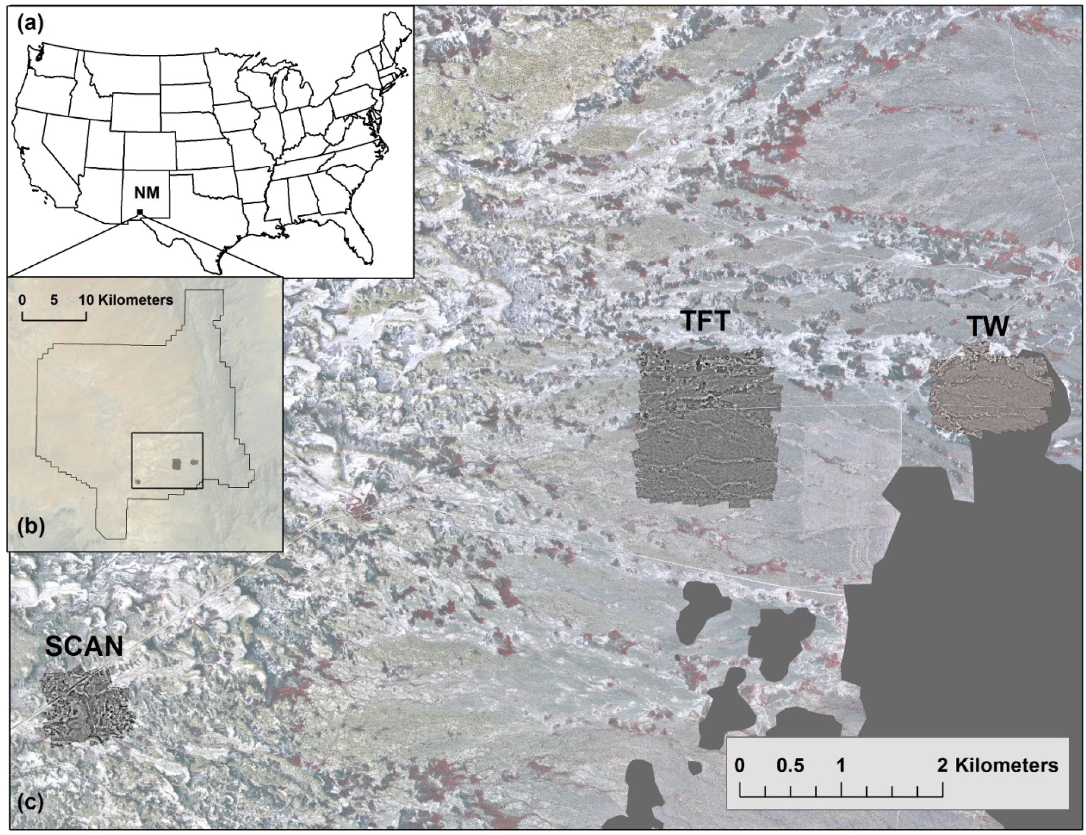
Figure 2.
Locations for UAS image acquisitions in southern New Mexico (a) at the Jornada Experimental Range (light grey outline) (b). The rectangle in (b) is shown in greater detail in (c) with the three UAS image mosaics (SCAN, TFT, TW) displayed over the WorldView-2 image. Dark grey areas in the WorldView-2 image are masked out areas of cloud and cloud shadow.
Table 1.
Image acquisition details.
Table 1.
Image acquisition details.
| Image type | Sites | Date | Number of UAS Images |
|---|
| World View-2 | Western Jornada | 26 October 2010 | |
| UAS Aerial | TW | 10 November 2010 | 160 |
| TW | 25 May 2011 | 160 |
| SCAN | 77 |
| TFT | 387 |
2.2. Image Processing
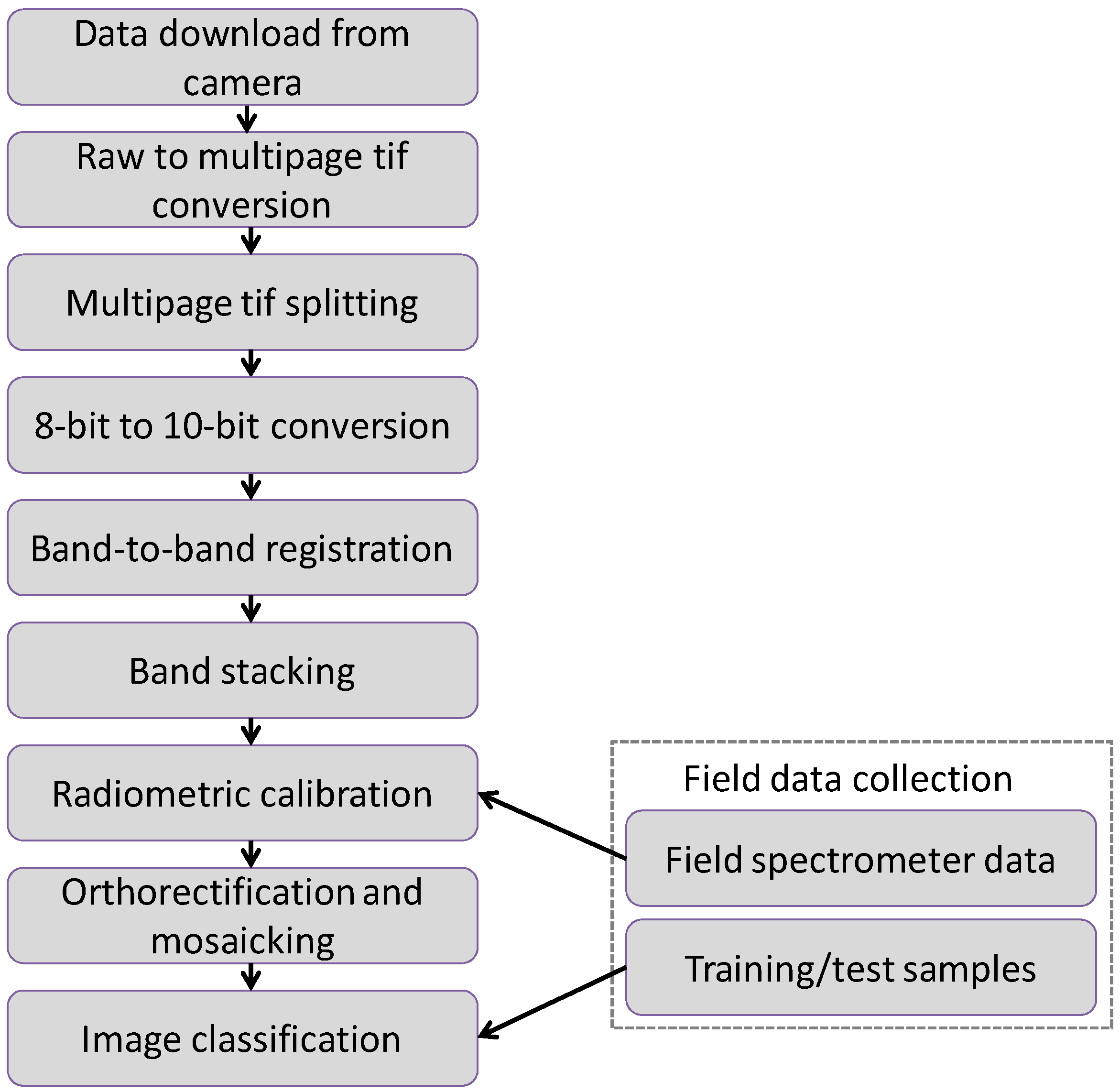
The image processing workflow from data acquisition through image classification is shown in
Figure 3. Each of the steps is described in detail in the following sections.
Figure 3.
Workflow for processing raw UAS-acquired MCA imagery into an orthorectified, radiometrically calibrated image mosaic and vegetation classification product.
Figure 3.
Workflow for processing raw UAS-acquired MCA imagery into an orthorectified, radiometrically calibrated image mosaic and vegetation classification product.
2.2.1. Data Import and File Conversion
The image data are stored in raw format on the six CF cards on the MCA camera. Data can be downloaded either by loading the CF cards in a card reader and copying the data, or by using the USB connection on the camera and downloading the data via an interface provided with the Tetracam software PixelWrench 2 (PW2). While relatively slow, the USB download is preferable in the field in order to minimize dust entering the interior of the camera, because the control boards are partially exposed when removing the CF cards. While most downloading occurs in the office, in some cases image quality needs to be checked in the field after the flights. We compared the times required for downloading using both methods.
The PW2 software provides a batch file conversion from raw to multipage TIF. While the multipage TIF file format allows for scrolling through the six image bands within the PW2 software, this file format is incompatible (either opening or importing) with image analysis programs commonly used with multispectral imagery (Erdas, ENVI, ArcGIS,
etc.). Only 3-band, 8-bit images can be exported from PW2. In order to access the bands in TIF format and preserve the 10-bit data range, we used the program Tiffsplitter 3.1 (
http://www.tiffsoftware.com) which has a batch process to split the multipage TIF files into the six bands in TIF format readable by other software.
2.2.2. Band-to-Band Registration and Bit Conversion
Although the image data are acquired in 10-bit raw format, the PW2 software cannot store 10-bit data in TIF format. Instead, for each band, the 10-bit data is distributed across the 3 bit planes (Red, Green, Blue) of the TIF file by dividing the original 10-bit value by 4 and storing that value in the Red and Green bitplanes, and the remainder of the division in the Blue bitplane. This allows for reconstructing the 10-bit values using the formula:
where
G and
B are the 8-bit values in the Green and Blue bitplanes. This conversion results in a panchromatic 16-bit TIF file.
The band-to-band registration is a crucial aspect of image pre-processing, because with six cameras, band mis-alignment can strongly affect spectral image analysis results. The PW2 software provides a band-to-band registration step as part of the raw to multipage TIF file conversion by using an alignment file that contains information about the translation, rotation, and scaling between the master and slave cameras. The process to determine the band alignments in PW2 consists of first determining rotation and scaling by measuring length and angle of a line between two target points on each respective master/slave band combination. In a second step, the translation is determined by calculating the X,Y positions for a single point on the master/slave band combination. The translation, rotation, and scaling information is stored in an alignment file that can be applied to a series of images. We determined that this band-to-band alignment method lacked robustness due to the paucity of points used to determine the offsets. The method resulted in relatively fair alignment at the center of the image, but poor alignment at the edges, most likely due to lens distortion and variability in alignment between the individual lenses and their sensors. However, since the band alignment is already part of the raw to multipage TIF file conversion, using PW2 is rather convenient and we wanted to compare the results with other approaches. In order to improve the alignment, we first tested a band-to-band registration approach based on 85 tie points between master and slaves. The resulting polynomial model was applied in batch processing mode to all images. While the results were superior to the PW2 method, band misalignments were still apparent and could potentially affect accuracy of image analysis results.
To further improve the band alignment, we developed a new automated band-to-band registration algorithm using a local weighted mean transform (LWMT), which is better able to compensate for locally varying pixel misalignments between bands than a polynomial approach. The algorithm automatically derives statistics for the mis-registration between the master (band 6) and the slaves (bands 1–5). The LWMT algorithm is based on the phase-correlation registration assessment method [
35]. First, the mis-aligment between bands is estimated across each image in 128 × 128 pixel blocks and compared to the reference band. This provides an estimate of the local variation of the registration. Next, outliers are filtered to remove locations where the registration estimate failed due to lack of features in the image. Finally, a local averaging operation is used to estimate the mis-alignment across the entire image. While it can be assumed that the band-to-band alignment does not change from image to image within the same flight, it is advantageous to assess the band mis-registration for a large number of images to reduce the random error in the registration estimate. In this study, the mis-registration estimate was further defined by averaging the mis-registration statistics of all 624 images in the dataset and applying the results in the band-to-band registration. Once the refined mis-registration estimate was complete, the registration correction was applied to each image using bilinear resampling. The LWMT algorithm is applied in a batch mode using parallel processing across multiple CPU cores for optimal use of the available computing power and to minimize processing time.
Registration results obtained from PW2 and the LWMT algorithm were evaluated using statistics evaluating pixel mis-alignment, spatial profiles, and visual assessments. After band co-registration, the bands were stacked using a batch processing procedure in Erdas modeler (Erdas, Inc., Norcross, GA, USA) to obtain a 6-band 10-bit image in ERDAS IMG file format for subsequent radiometric calibration.
2.2.3. Radiometric Calibration
For radiometric calibration, we used two calibration targets (each 2.4 m × 2.4 m), painted with black flat paint and white paint. The average reflectance of the black and white targets was 0.02 and 0.85 respectively. The black and white targets were constructed out of eight 1.2 m × 1.2 m panels of whiteboard that were laid over a leveled PVC frame to raise the targets above the ground. The frame and targets are sufficiently lightweight to be easily transported and assembled for use on multiple UAS flights. An ASD FieldSpec Pro (ASD Inc., Boulder, CO, USA) was used to obtain radiance measurements of the calibration targets and selected vegetation and soil targets during the 10 November 2010 UAS flight. Target reflectance was calculated using measurements of irradiance acquired over a Spectralon® panel. The FieldSpec Pro acquires data in multiple narrow bands (3–10 nm spectral resolution) with a spectral range of 350–2,500 nm. These near-continuous data were resampled using a weighted mean based on the relative spectral response of each of the six MCA bands. An empirical line calibration method [
36] was used to derive coefficients to fit the digital numbers of the MCA imagery to the ground measured reflectance spectra.
Test flights prior to the November 2010 image acquisitions had been conducted to determine the optimum exposure settings. In spite of this, variations in reflectance from image to image remained due to illumination and viewing geometry. For this study, we did not attempt to derive parameters for the Bidirectional Reflectance Distribution Function (BRDF), because it would add considerable time and complication to the processing and would not be a feasible option for multiple UAS image acquisitions. The images also had a relatively strong anisotropic vignetting effect. The PW2 software has a vignetting correction function that was applied during the file conversion, however, the correction does not handle anisotropic effects well, and some vignetting effects remained. We determined that additional color balancing was necessary to produce a seamless mosaic, and an image dodging process was applied in Erdas during the mosaicking process. The dodging process uses grids to localize problem areas within an image (dark corners due to vignetting, hotspots), and applies a proprietary algorithm for color balancing. While this process was successful in eliminating the remaining vignetting effects, this manipulation affected the radiometric values of the images.
For that reason, we tested two methods of applying the empirical line calibration for radiometric correction. For the first radiometric calibration method (RC-IND), we obtained digital numbers for the black and white targets from a single image, then applied the radiometric correction to every individual image, and subsequently mosaicked the images, using an image dodging approach to produce a seamless mosaic. For the second radiometric calibration method (RC-MOS), we first mosaicked the un-calibrated images using the same image dodging method, then obtained digital numbers from the black and white targets from the image mosaic, and subsequently applied the radiometric correction to the image mosaic. A validation of the two methods was performed by evaluating the correlation between the ground reflectance acquired with the FieldSpec and reflectance values derived from the RC-IND and RC-MOS image mosaics for vegetation and soil patches.
2.2.4. Orthorectification and Mosaicking
The same approach we developed for orthorectification and mosaicking of the UAS-acquired RGB images with the Canon camera was applied to the processing of the MCA imagery. Details have been described elsewhere [
8,
29]. Briefly, the process used automatic tie point detection applied to a 3-band image, and a custom image matching algorithm (PreSync) applied to the UAS imagery and a 1 m resolution digital ortho image. A 5 m resolution digital elevation model (DEM) derived from Interferometric Synthetic Aperture Radar (IfSAR) data provided elevation information. Although exterior orientation data (position, attitude) from GPS and Inertial Measurement Unit (IMU) are provided by the UAS’ flight computer, the data have a low level accuracy that requires refinement. This was achieved in PreSync using an iterative optimization approach involving initial tie point alignment, rigid block adjustment, individual image adjustment, and realignment of tie points. Additional inputs included the camera’s interior orientation parameters (radial lens distortion, principal points, focal length) derived from a camera calibration procedure performed using PhotoModeler (Eos Systems, Inc., Vancouver, Canada). The output of the PreSync process was a data file with improved exterior orientation parameters and tie points with X,Y,Z information, which were used as input for the orthorectification and mosaicking process in Leica Photogrammetry Suite (LPS) (Erdas, Inc., Norcross, GA, USA). Our approach minimizes or eliminates the need for manual input ground control points, which commonly increase the cost and time of image processing. Geometric accuracies achieved with this approach have resulted in root mean square errors (RMSE) of 0.6–1.1 m for mosaics composed of 150–250 images with a GSD of 6 cm [
8]. For this study, we evaluated the geometric accuracy of the image mosaic by comparing target coordinates acquired with real time kinematic differential GPS with image coordinates.
2.3. Field Measurements
We collected training and validation samples for the vegetation classification of the TW image within two weeks of the UAS flight. Previous tests of different methods for training sample collection for very high resolution UAS imagery have shown that on-screen digitizing of the samples over the image mosaic was most suitable for an object-based image classification [
9]. This approach was used here, and the samples were selected in the field by walking the entire study area and selecting samples based on proportional cover of individual species. For shrubs, the samples consisted of the entire shrub, while for grasses, patches of a minimum of 0.2 m
2 were selected. We collected a total of 1,083 samples (0.2% of all image objects) for eight vegetation species (sample numbers in brackets): honey mesquite (
Prosopis glandulosa Torr.) (shrub) (184), Sumac (
Rhus L.) (shrub) (67), Creosote (
Larrea tridentata (DC.) Coville) (shrub) (331), Tarbush, (
Flourensia cernua DC. ) (shrub) (96), Mariola (
Parthenium incanum Kunth) (shrub) (137), Broom snakeweed (
Gutierrezia sarothrae (Pursh) Britton&Rusby) (sub-shrub) (165), Tobosa grass (
Pleuraphis mutica Buckley) (grass) (57), Bush muhly (
Muhlenbergia porteri Scribn. Ex Beal) (grass) (46), as well as bare ground, and sparse vegetation on bright and dark soils. Using a random selection process, half of the samples were used to train the classifier, and half were retained for accuracy assessment.
2.4. Image Classification
An object-based image classification (OBIA) approach using eCognition 8.64 (Trimble GeoSpatial, Munich, Germany) was used. OBIA is highly suitable for very high resolution imagery, where pixel-based classification is less successful due to the high spatial variability within objects of interest. In its most basic form, OBIA consists of classification of image objects, but more commonly a recursive approach is implemented using image segmentation, classification of image objects, merging of objects, re-segmentation and re-classification using a combination of expert knowledge, fuzzy classification, and the incorporation of spectral, spatial, and contextual features for extraction of meaningful image objects [
37]. Rule sets are saved as process trees and can be applied and adapted to other images. In this case, we used a rule set developed for the image mosaic acquired over the same site with the Canon camera. Adaptations detailed below were made to account for the greater number of spectral bands and difference in spatial resolution. The OBIA steps were as follows:
- (1).
The mosaic was segmented at two scales based on visual assessment: a finer multi-resolution segmentation (scale parameter 20, color/shape 0.9/0.1, compactness/smoothness 0.5/0.5), and a coarser spectral difference segmentation (max spectral difference 100) to aggregate adjacent objects with similar spectral information while retaining spectrally unique shrub and grass patches.
- (2).
A rule-based classification was used to define the classes shadow, vegetation, and bare/sparse vegetation in a masking approach. Brightness was used to define shadow, and the normalized difference vegetation index (NDVI) was used to define the vegetation and bare/sparse vegetation classes.
- (3).
Objects within the vegetation and bare/sparse vegetation classes were merged and re-segmented using a combination of chessboard and spectral difference segmentation to better delineate shrub canopies and patches of bare, grass, and sparse vegetation.
- (4).
A rule-base classification was used for the bare/sparse vegetation class to differentiate between bare, sparse vegetation on bright soils, and sparse vegetation on dark soils using a threshold for the mean of the blue band.
- (5).
In the vegetation class, the re-segmentation clearly defined individual shrub canopies and grass patches for further classification. The field-collected samples for the vegetation classes were used as training samples for a nearest neighbor classification, using the most suitable features determined from the following two-step feature selection process.
For each sample segment, we extracted information for 15 features: the means and ratios of the six bands, NDVI, area, and roundness. We used predominantly spectral features, because aside from the Broom snakeweed, which is relatively small and round, all other shrub and grass species had no discernable spatial features. The feature selection process consisted of (1) a Spearman’s rank correlation analysis to retain only those features with correlation coefficients smaller than 0.9, and (2) a decision tree analysis using CART (Salford Systems, San Diego, CA, USA ) [
38] to determine the optimum features based on the variable importance scores of the primary splitter in the decision tree. The variable importance scores reflect the contribution of the features in predicting output classes and range from 0 to 100. This two-step feature selection method proved to be an efficient and objective method of reducing input features and selecting the most suitable features based on training sample data for other UAS-acquired imagery [
9]. Using half of the field-collected samples, we conducted a classification accuracy assessment to obtain overall, producer’s, and user’s accuracies, and the Kappa index [
39].
2.5. Comparison with WorldView-2 Data
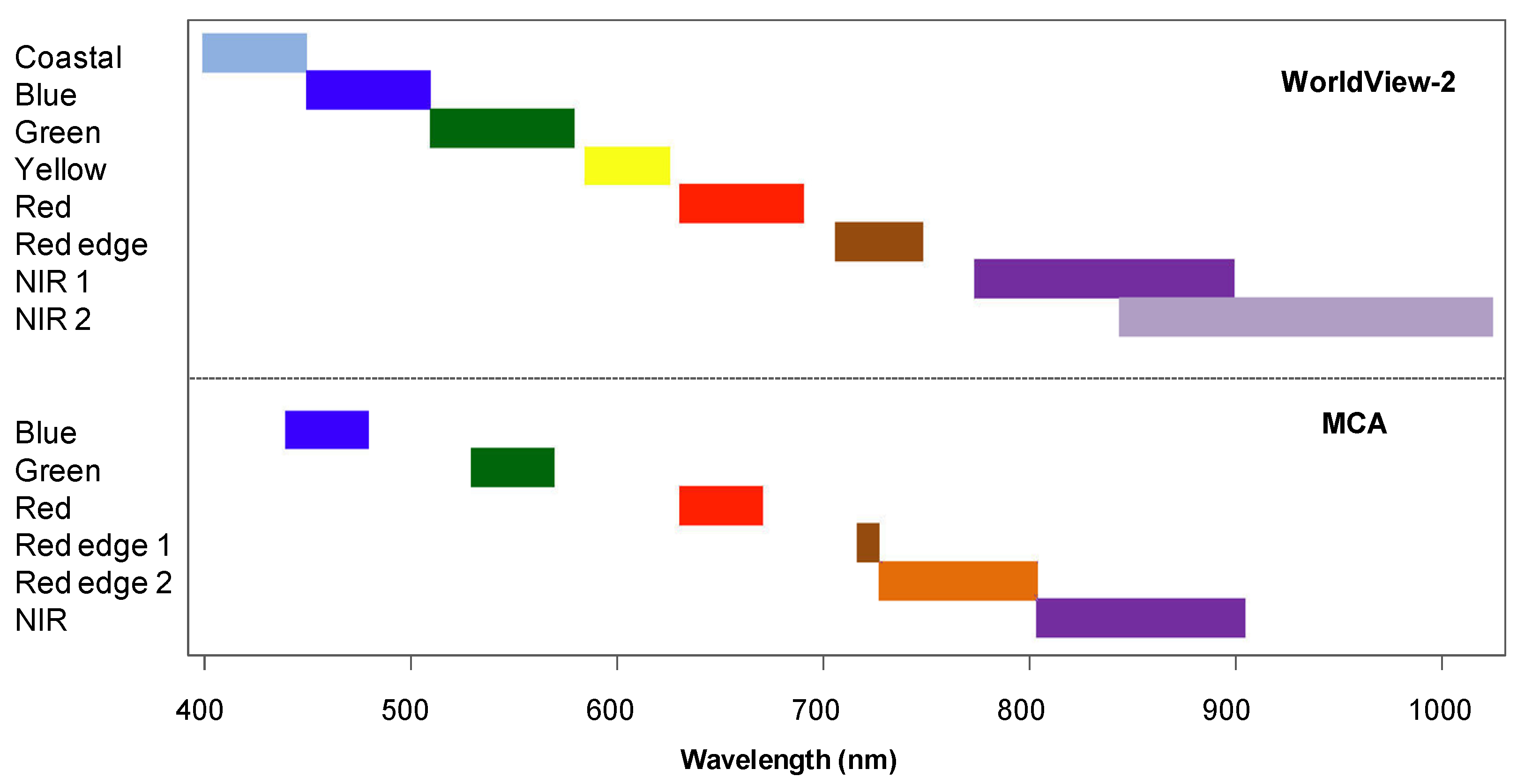
The WorldView-2 satellite acquires imagery in one panchromatic and eight multispectral bands ranging from 425 nm to 950 nm (center wavelengths). Spatial resolution is 50 cm for the panchromatic and 2 m for the multispectral bands. The band widths and band distribution for the MCA and WorldView-2 multispectral data (
Figure 4) are sufficiently similar to allow for a comparison of the spectral information acquired from both sensors. The WorldView-2 multispectral image was orthorectified using a 1 m resolution digital ortho image mosaic and a 5 m resolution Interferometric Synthetic Aperture Radar (IfSAR) DEM. The image was radiometrically and atmospherically corrected using ATCOR2 for Erdas (Geosystems GmbH, Germering, Germany), employing the coefficients provided by DigitalGlobe (Longmont, CO, USA) [
40].
With both image products corrected to reflectance, we compared spectral information for bare soil, sparse vegetation, and six vegetation species (Mesquite, Sumac, Creosote, Mixed grass, Dense Tobosa grass, and Sparse Tobosa grass) for the following bands: blue, green, red (for both sensors), red edge (WorldView-2) vs. red edge 1 (MCA), and NIR 1 (WorldView-2) vs. NIR (MCA). The objective was not to conduct an in-depth comparison, but rather to evaluate the spectral responses of vegetation and soil in the different bands graphically, and to determine the correlation of spectra for the sensors to draw general conclusions about the potential for upscaling of the MCA imagery in future studies.
Figure 4.
MCA and WorldView-2 band widths (full-width at half maximum) and band distribution. For this study, we compared vegetation and soil spectra in the blue, green, and red bands of both sensors, the red edge (WorldView-2) vs. red edge 1 (MCA), and the NIR 1 (WorldView-2) vs. NIR (MCA) bands.
Figure 4.
MCA and WorldView-2 band widths (full-width at half maximum) and band distribution. For this study, we compared vegetation and soil spectra in the blue, green, and red bands of both sensors, the red edge (WorldView-2) vs. red edge 1 (MCA), and the NIR 1 (WorldView-2) vs. NIR (MCA) bands.
3. Results and Discussion
3.1. Assessment and Efficiency of Processing Workflow
A breakdown of the time required for the batch processing steps from data download to radiometric correction is shown in
Table 2. Details of the remaining image processing steps (orthorectification, mosaicking, classification) are described in subsequent paragraphs. All processing was performed on a workstation with 4 GB of RAM and two dual-core 2.6 GHz processors. Copying the CF cards by removing them from the camera was considerably faster (0.2 s/band, including switching the cards) than using the USB download (2.6 s/band [not shown in
Table 2]), which was relatively slow due to the USB 1.1. Version. For 624 images, using the USB download took 2 h, 29 min. In most cases, this may not be a limiting factor, as this process runs unassisted, but if the images require a quick assessment after the flight to determine image quality, copying the CF cards is more efficient.
Both the raw to multipage TIF conversion and the multipage TIF splitting were run in batch processing mode and required only initiating the process in the respective programs (PW2 and Tiffsplitter). The band-to-band registration and bit conversion step listed in
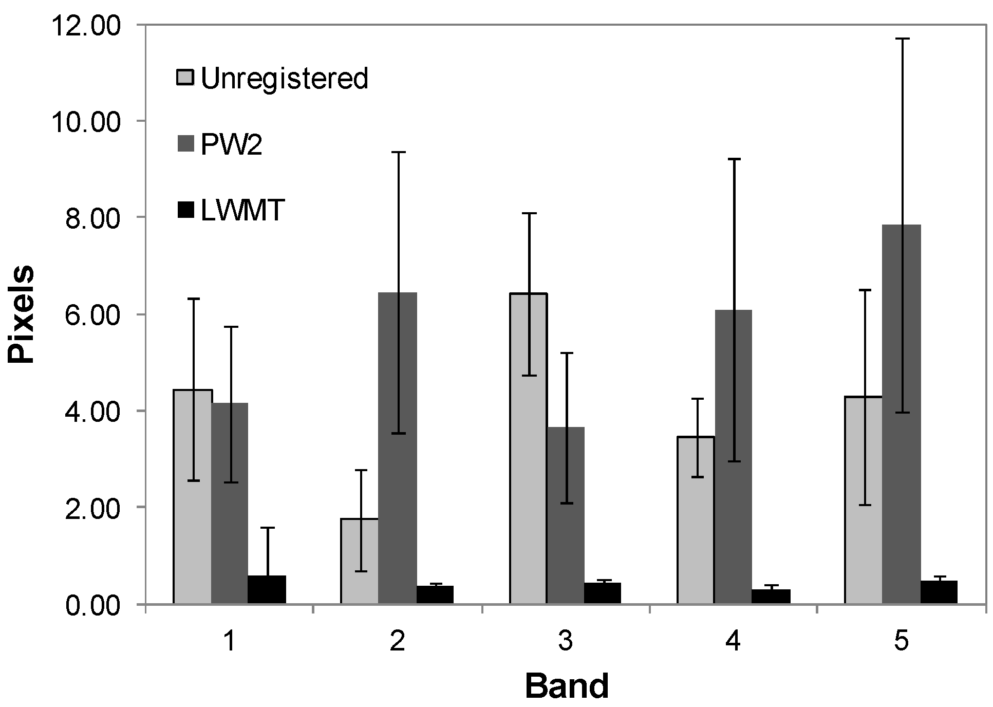
Table 2 is for the LWMT method we used for this dataset. The band co-registration method implemented in PW2 is part of the raw to multipage TIF conversion algorithm, and thus would not increase processing times. However, the results of the LWMT band-to-band registration were far superior to the process implemented in PW2, and therefore LWMT was the preferred method. A comparison of the statistics for the pixel mis-alignment of the unregistered bands, and after band-to-band registration using PW2 and LWMT demonstrated a considerably lower band mis-alignment for the LWMT method with a mean of 0.5 pixels compared to the PW method, which had relatively poor results and a greater variation for the bands (
Figure 5). No obvious systemic errors were observed in the band co-registration.
Table 2.
Time required for multispectral image batch processing steps per band, per image, and for the 624 images from the May 25, 2011 flight.
Table 2.
Time required for multispectral image batch processing steps per band, per image, and for the 624 images from the May 25, 2011 flight.
| Processing step | Per Band
(s) | Per Image
(s) | 624 Images
(h:min) |
|---|
| Data download from camera (copy CF cards) | 0.2 | 1.2 | 0:12 |
| Raw to multipage TIF conversion | 1.1 | 6.6 | 1:08 |
| Multipage TIF splitting | 0.2 | 1.4 | 0:14 |
| Band-to-band registration and bit conversion | 1.6 | 9.6 | 1:39 |
| Band stacking | | 4.0 | 0:41 |
| Radiometric correction (RC-IND method) 1 | | 5.0 | 0:52 |
| Total | 3.1 | 27.8 | 4:49 |
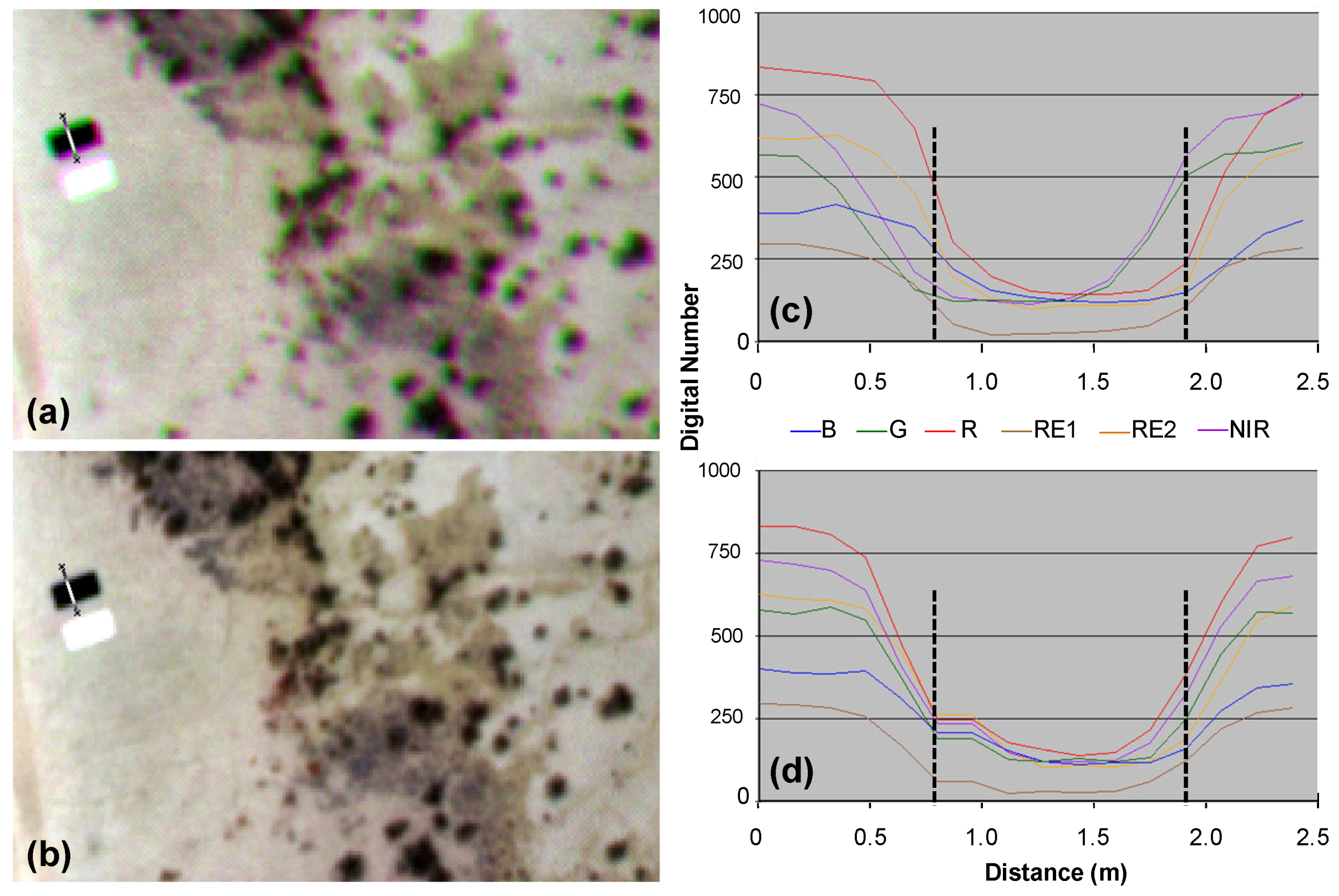
The band-to-band registration results were also examined visually and using spatial profiles (
Figure 6). Using the PW2 band-to-band registration approach resulted in noticeable halos around image objects (shrubs and targets) and noise in the homogenous portions of the image (
Figure 6(a)). With the LWMT approach, the halos were eliminated, and the noise in the soil and grass patches was reduced (
Figure 6(b)). The band mis-alignment in PW2 was obvious when examining the spatial profile across the black radiometric target (
Figure 6(c)), while in the LWMT approach, the bands were well aligned (
Figure 6(d)).
Figure 5.
Mean and standard deviations of pixel mis-alignment between bands 1–5 (slaves) compared to band 6 (master) for unregistered bands, and band-to-band registration approaches using PW2 and local weighted mean transform (LWMT).
Figure 5.
Mean and standard deviations of pixel mis-alignment between bands 1–5 (slaves) compared to band 6 (master) for unregistered bands, and band-to-band registration approaches using PW2 and local weighted mean transform (LWMT).
Figure 6.
Images and spatial profiles depicting comparison of band-to-band registration using the approach implemented in PW2 and the LWMT. The PW2 approach (a) resulted in halos around shrubs and target; the LWMT approach (b) had improved band alignment. The spatial profiles (2.5 m long) for PW2 (c) and LWMT (d) were taken across a black radiometric target. The dotted lines in and indicate the edges of the black target. The improved band-to-band alignment for the LWMT approach is apparent by the lack of halos around shrubs and targets, and the reduced noise in the soil background. The band order in the images is Near Infrared, Red, Green.
The band-to-band alignment is expected to remain relatively constant unless one of the camera’s sensors is physically removed or one of the filters is changed, which would necessitate a new mis-registration assessment. To date, we have applied the band-to-band registration approach using the same statistics on data acquired during subsequent flights with equally good band registration.
Having close alignment for the bands is crucial for subsequent image analysis, especially when spectral signatures for specific vegetation species are extracted. Many of the shrubs are relatively small, and if the bands are not well aligned, the signatures may include pixels not belonging to the shrub canopy. Using a band-to-band registration method with sub-pixel accuracy ensures high accuracy results.
3.2. Radiometric Calibration Results
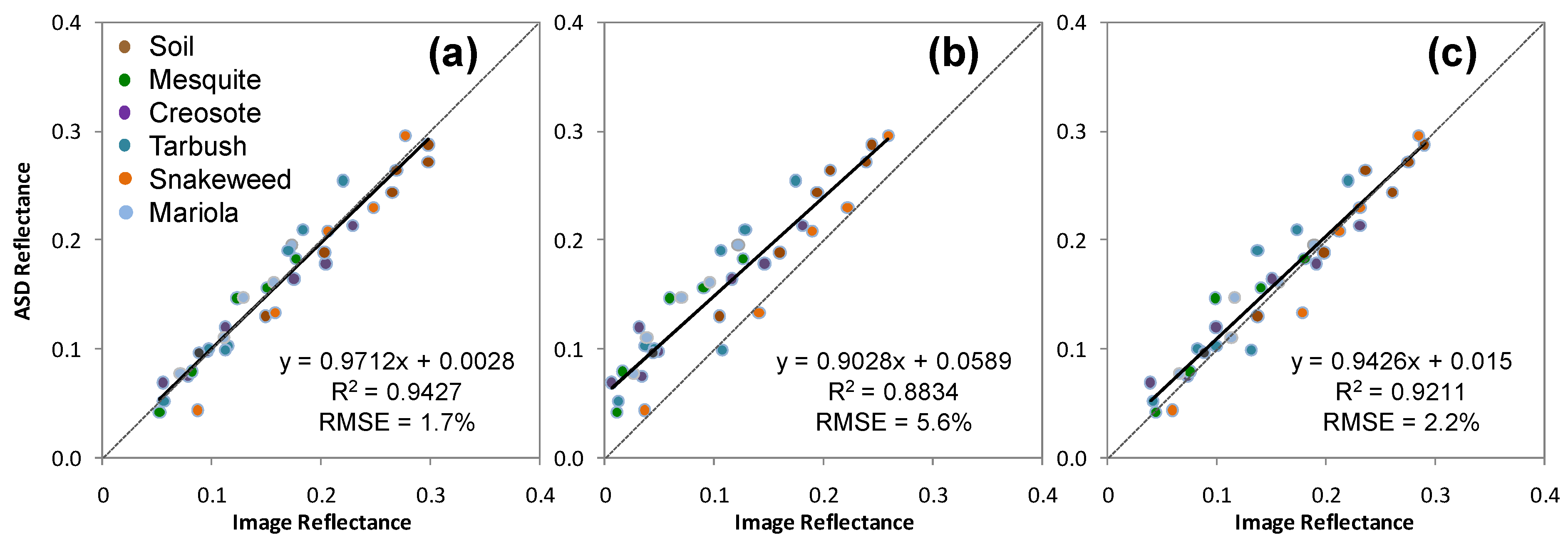
The validation of the radiometric calibration showed high correlation (R
2 = 0.94, RMSE = 1.7%) between ground reflectance and image reflectance after applying the empirical line calibration to the single image covering the calibration targets (
Figure 7(a)). The agreement between image reflectance and ground reflectance was inferior for the RC-IND method (
Figure 7(b)) than the RC-MOS method (
Figure 7(c)). The larger error in the RC-IND method was likely associated with the image-to-image differences in illumination and viewing geometry, and the vignetting effects.
Figure 7.
Evaluation of radiometric calibration depicting correlations between ground reflectance from the field spectrometer and MCA image reflectance for 5 shrub species and bare soil for 6 spectral bands. In (a), reflectance values for a single image are depicted, in (b) the image reflectance values were extracted from a mosaic composed of individually radiometrically calibrated images (RC-IND method), and in (c), radiometrically un-calibrated images were mosaicked first, followed by radiometric correction of the mosaic (RC-MOS method).
When the empirical line calibration corrections were applied to each image, the underlying image-to-image variations remained, resulting in less than accurate reflectance values. In the RC-MOS method, a seamless mosaic was produced before radiometric correction, and the vignetting effects and image-to-image variations were largely eliminated before the radiometric correction was applied to the image mosaic. As mentioned, we did not attempt a BRDF correction for this dataset, because obtaining the required parameters can be time consuming and would add considerably to the image processing time. However, BRDF correction would likely reduce the image-to-image variations we observed, and potential methods adapted to UAS-acquired imagery have been described elsewhere [
22,
41].
For our purposes, we concluded that the RC-MOS method yielded satisfactory results, and in addition resulted in a decrease in processing time. Compared to the RC-IND method, which required 5 s/image or 52 min for 624 images to apply the empirical line calibration to each image (
Table 2), the MOS method only required a total of 8 min to apply the calibration to all three image mosaics. Note that the determination of the calibration coefficients was not included in the time estimate in
Table 2, but would add approximately 30 min to the total processing time.
The orthorectification and mosaicking was largely identical to the process we had developed for the imagery acquired with the Canon camera [
8]. In some images, additional tie points were required to achieve a satisfactory image to image alignment. The PreSync portion took the bulk of the processing time at 100 s/image. The process was run overnight, and the general turnaround time for producing an orthorectified image mosaic was 1–2 days, depending on the number of images. The extent of the orthomosaics was 9,187 × 9,778 pixels (TFT), 9,318 × 5,343 pixels (TW), and 6,268 × 5,417 pixels (SCAN). A comparison of the coordinates of 12 targets visible in the TW mosaic and measured with real time kinematic differential GPS resulted in an RMSE of 0.84 m, reflecting the kind of accuracy we generally achieve with the orthorectification approach without the use of ground control points. Although the UAS does not have a highly accurate GPS/IMU, and the absolute accuracy of the image coordinates at time of capture is relatively poor, the image matching procedure to a DOQ in PreSync compensates, resulting in relatively good internal geometric accuracies of the orthomosaics.
3.3. Image Classification and Accuracy
The two-step feature selection process reduced the 15 input features to eight optimum features based on the variable importance scores of the primary splitter in the decision tree. The optimum features were (feature followed by variable importance score in brackets): NDVI (100), Mean Near Infrared (93.68), Ratio Blue (90.93), Ratio Green (59.19), Mean Red (40.15), Mean Blue (32.31), Area (31.95), and Ratio Red edge 1 (28.45). The feature Area was only associated with the Broom snakeweed class in the decision tree. This was consistent with our expectations and with previous studies where Area had been an important feature associated with this shrub. Based on this information, we chose the seven spectral features for all classes, and in addition included the feature Area for the Broom snakeweed class.
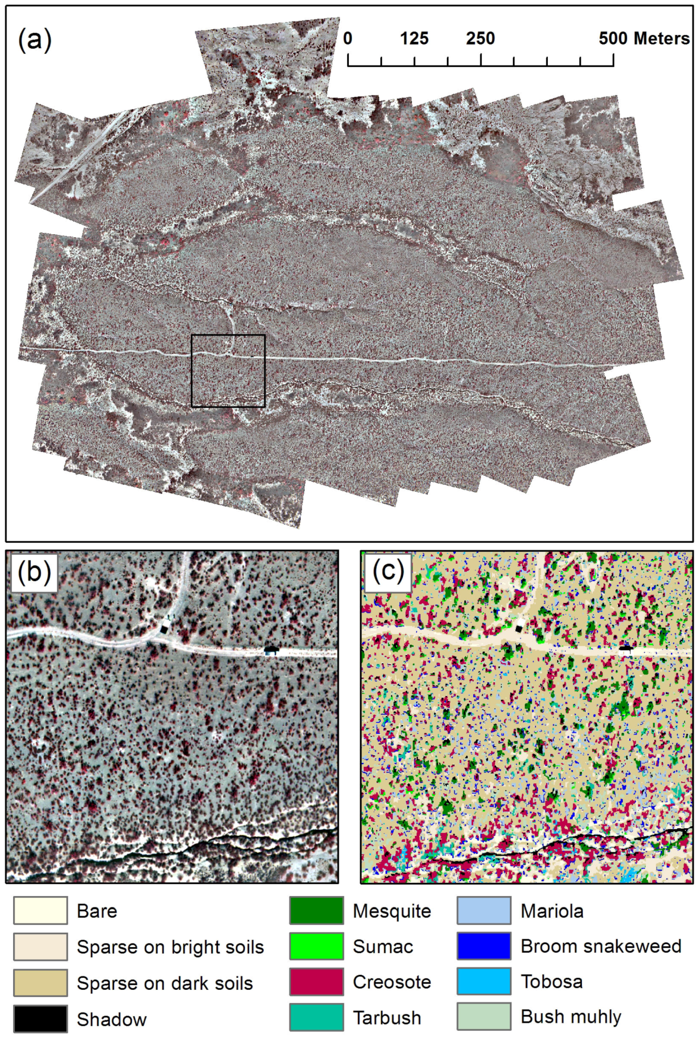
The resulting classification provided fine scale detail, and a visual assessment showed good differentiation for the chosen classes (
Figure 8). Overall classification accuracy for the vegetation classes was 87%, with producer’s accuracies ranging from 52% to 94%, and user’s accuracies from 72% to 98% (
Table 3). The omission errors for Tarbush were mostly due to confusion with Creosote due to spectral similarity. Likewise, there was confusion between Sumac and Mesquite. Closer inspection of the mislabeled objects showed that the errors could be attributed to a canopy segmentation that was less than ideal for selected objects for these species. Due to the structure of the Mesquite and Sumac shrubs, brighter and darker portions of the canopy occurred in different segments instead as a single segment, which resulted in the omission errors in the Sumac class.
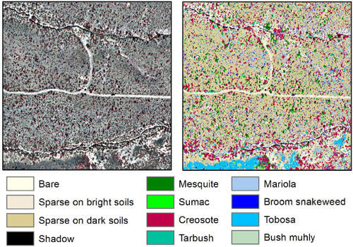
Figure 8.
UAS image mosaic of TW site (a), detailed view of a 130 m × 130 m area in the black box (b), and vegetation classification (c).
Figure 8.
UAS image mosaic of TW site (a), detailed view of a 130 m × 130 m area in the black box (b), and vegetation classification (c).
A good segmentation is crucial for a highly accurate classification, and while the segmentation quality was good overall, and shrubs were delineated well in the remaining classes, the canopy structure and brightness variations of Mesquite and Sumac led to a less suitable segmentation for some shrubs in these classes. Possible improvements would include editing of selected segments to merge adjacent segments in the same shrub canopy, which would likely improve the accuracy results. For this study, however, we wanted to assess the classification accuracy without editing in order to evaluate the rule set.
An OBIA rule set has the potential to be applied repeatedly to image mosaics of the same area, or, with adjustments, to mosaics of other areas. Transferring rule sets reduces the time spent on image classification, increases efficiency, and is objective [
9,
42]. For this study, we adapted a rule set from an image mosaic of the same area, but acquired with the Canon camera. The major steps of analysis remained the same: segmentation at two scales, masking of shadow, vegetation, and bare/sparse vegetation, merging and re-segmentation of the vegetation and bare/sparse vegetation classes, followed by sample selection, feature selection and nearest neighbor classification. Edits were required for the segmentation parameters, the threshold values in the masking process, choice of features and site-specific samples. These edits were minimal compared to developing a completely new rule base, and the resulting classification accuracy demonstrated that this was a viable approach for UAS-based multispectral image classification.
Table 3.
Error matrix for classification of TW site. Rows represent classification data, columns represent reference data. Values are in pixels. Bold numbers are correctly identified pixels.
Table 3.
Error matrix for classification of TW site. Rows represent classification data, columns represent reference data. Values are in pixels. Bold numbers are correctly identified pixels.
| Tarbush | Broom Snakeweed | Creosote | Bush Muhly | Mariola | Mesquite | Sumac | Tobosa |
|---|
| Tarbush | 1,047 | | 140 | 68 | | | | |
| Broom snakeweed | 13 | 1,129 | 28 | 65 | 205 | | | 99 |
| Creosote | 520 | | 11,810 | 485 | 38 | 1,865 | 184 | |
| Bush muhly | 293 | 10 | 90 | 3,687 | 322 | | | 687 |
| Mariola | 23 | 281 | 75 | 345 | 3,353 | | 38 | |
| Mesquite | 132 | | 399 | | | 15,840 | 776 | |
| Sumac | | | | | | 37 | 956 | |
| Tobosa | | 150 | | | | | | 9,776 |
| Producer’s Acc. (%) | 52 | 72 | 94 | 79 | 86 | 89 | 49 | 93 |
| User’s Acc. (%) | 83 | 73 | 79 | 72 | 81 | 92 | 96 | 98 |
| Overall Acc. (%) | 87 | | | | | | | |
| Kappa index | 0.83 | | | | | | | |
3.4. Spectral Reflectance Data from MCA and WorldView-2
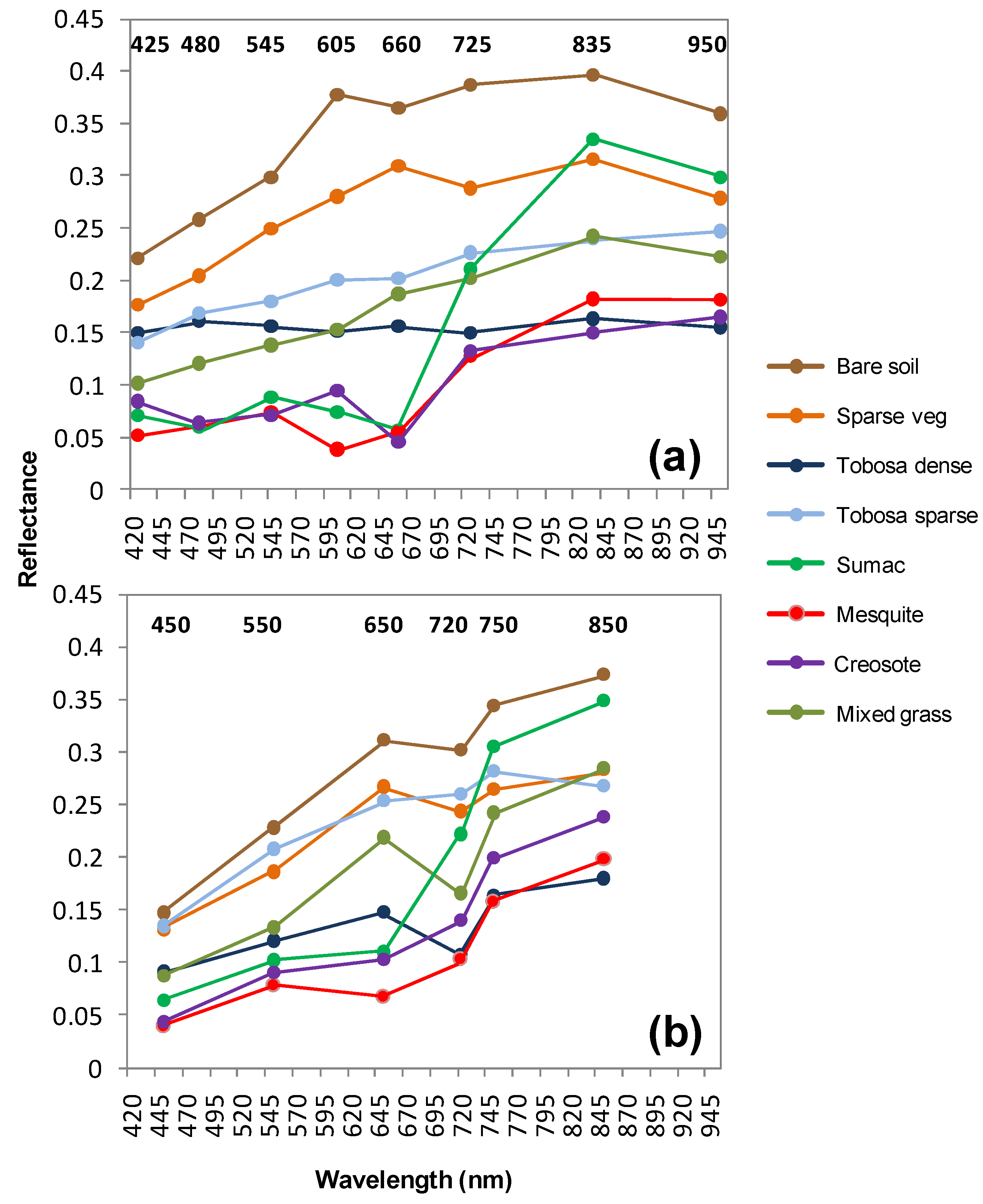
The comparison of the spectral reflectance data extracted from the MCA image mosaic and the WorldView-2 satellite image over the TW site showed relatively good agreement for the spectral responses of the vegetation and soil targets (
Figure 9 and
Figure 10). Most of the targets showed similar spectral responses for the two sensors, although some differences were apparent, most noticeably lower reflectance values for Tobosa sparse compared to Sparse vegetation in the WorldView-2 image (
Figure 9(a,b)). In general, the correlation of spectra for the two sensors was high, with somewhat lower reflectance values for the WorldView-2 image than the MCA image for the same target (
Figure 10). This can likely be attributed to the fact that although the ranges and centers of the sensors’ wavelengths were sufficiently close to draw comparisons, they were not identical (
Figure 4). Other sources of the variation in the reflectance values for the two sensors may include the different methods for calculating reflectance, as well as the resolution difference (14 cm for the MCA, 2 m for the WorldView-2). For small shrub species that are at the edge of the detection limit in the satellite image (
i.e., Creosote), discrepancies in reflectance may arise. This was reflected in the relatively low R
2 value for Creosote (
Figure 10). We were also somewhat limited in selecting suitable targets on the WorldView-2 image, because approximately ¾ of the TW site was occluded by cloud and cloud shadow in the satellite image.
Nevertheless, the data were sufficient to demonstrate the potential for either using the MCA data for ground truth of WorldView-2 data, or for upscaling fine detail information in the MCA imagery to larger areas using the satellite imagery. This could be accomplished by using the UAS to fly over key areas to capture detailed information for dominant vegetation communities, so that landscape scale mapping could be conducted using the WorldView-2 image.
Figure 9.
Comparison of spectral reflectance data for eight vegetation/soil targets extracted from WorldView-2 (a) and MCA (b). Five bands were compared (Blue, Green, Red, Red edge, Near Infrared).
Figure 9.
Comparison of spectral reflectance data for eight vegetation/soil targets extracted from WorldView-2 (a) and MCA (b). Five bands were compared (Blue, Green, Red, Red edge, Near Infrared).
4. Conclusions and Future Work
In this paper, we have described an efficient workflow for processing multispectral imagery acquired with an unmanned aircraft into orthorectified, radiometrically calibrated image mosaics for subsequent vegetation classification. We identified several challenges in the process, including file format incompatibilities, as well as software and camera limitations. There are few multispectral cameras available that are light weight enough for use on small UAS, and there is a need for high quality multispectral sensors as well as workflows that support fast turnaround times for quality remote sensing products. We envision that the limitations we discovered and the described solutions may lead to future improvements in software and hardware.
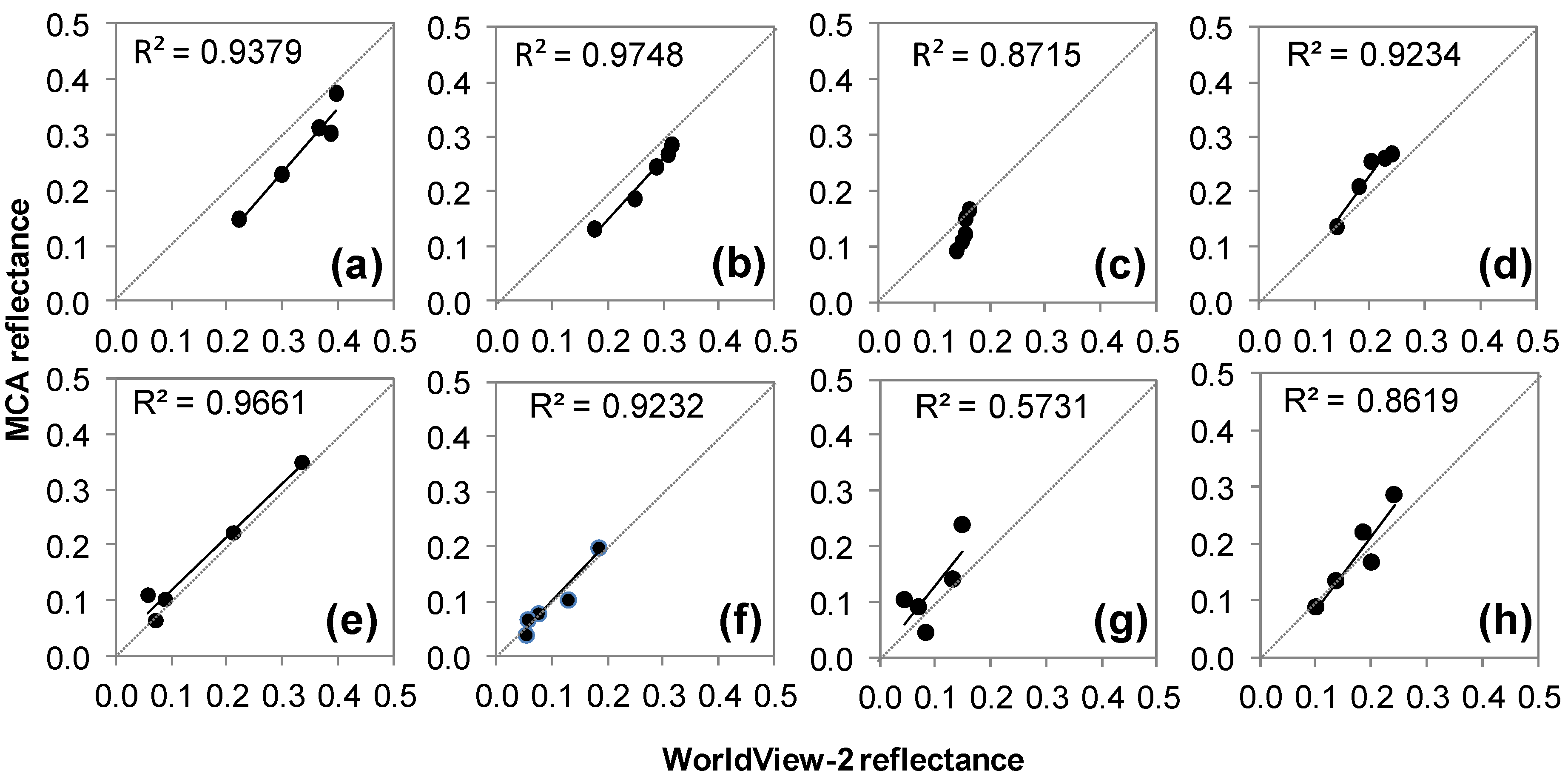
Figure 10.
Correlation of reflectance measurements for eight vegetation/soil targets extracted from WorldView-2 and MCA in the five bands that were compared (Blue, Green, Red, Red edge, Near Infrared). The graphs depict: Bare soil (a), Sparse vegetation (b), Tobosa dense (c), Tobosa sparse (d), Sumac (e), Mesquite (f), Creosote (g), and Mixed grass (h).
We developed several automated batch processing methods for file conversion, band-to-band registration, and radiometric correction, and these batch processes are easily scalable to larger number of images. The band-to-band-registration algorithm greatly improved the spectral quality of the final image product, leading to better agreement between ground- and image-based spectral measurements, especially for small shrub canopies. Deriving radiometric calibration coefficients from the image mosaic resulted in higher correlations between ground-and image-based spectral reflectance measurements than performing radiometric corrections on individual images. An orthorectified image mosaic can generally be produced in a two-day turnaround time, taking into account approximately five hours for the pre-processing steps, and the remainder for the orthorectification and mosaicking step.
For the vegetation classification, we were able to use an OBIA rule set previously developed for imagery acquired with the Canon camera over the same site. This approach saved time, and we plan to evaluate the applicability of this rule set for future image acquisitions, both for the same area and other sites. Based on experiences with transferability of rule sets for UAS images acquired with the Canon camera, we expect that the segmentation parameters and general processing steps (initial segmentation, rule-based classification, re-segmentation, merging, nearest neighbor classification) will remain the same, with changes required for specific thresholds and site-specific training samples.
Our comparison of vegetation and soil spectral responses for the airborne and WorldView-2 satellite data demonstrate potential for conducting multi-scale studies and evaluating upscaling the UAS data to larger areas, and future studies will investigate these aspects. In addition, we are currently acquiring multi-temporal multispectral UAS imagery for use in change detection studies.


