Abstract
The fraction of vegetation cover (FVC) is often estimated by unmixing a linear mixture model (LMM) to assess the horizontal spread of vegetation within a pixel based on a remotely sensed reflectance spectrum. The LMM-based algorithm produces results that can vary to a certain degree, depending on the model assumptions. For example, the robustness of the results depends on the presence of errors in the measured reflectance spectra. The objective of this study was to derive a factor that could be used to assess the robustness of LMM-based algorithms under a two-endmember assumption. The factor was derived from the analytical relationship between FVC values determined according to several previously described algorithms. The factor depended on the target spectra, endmember spectra, and choice of the spectral vegetation index. Numerical simulations were conducted to demonstrate the dependence and usefulness of the technique in terms of robustness against the measurement noise.
1. Introduction
The spatio-temporal distribution of biophysical parameters on land surfaces has been retrieved from remotely sensed surface reflectances [,]. The fraction of vegetation cover (FVC) is the fraction of the horizontally projected area occupied by green vegetation, which is estimated to quantify the horizontal spread of vegetation on the subpixel level. FVC provides useful information for monitoring changes in the forest [] or land use [], and it guides policy development decisions []. FVC estimates at the continental and larger scale have been used as input parameters to describe surface processes in climate models [,].
Several types of algorithm have been introduced and developed for estimating FVC from multispectral and hyperspectral data. Among them, techniques based on linear mixture models (LMM) have been employed most frequently [,,,,,] The framework of these models was proposed by [] and extracts useful information in terms of the fractional abundances of spectra corresponding to pure components (endmembers) within a certain area. The LMM algorithms have been developed in several studies [,] to analyze surface materials or minerals [,], classify [,], and inform other environmental studies []. FVC retrieval techniques have been facilitated by unmixing an LMM to compute the weights of vegetation endmembers []. Subsequently, numerical inversion of a radiative transfer model [,] and signal processing approaches, including neural networks [,], have been applied to FVC estimation.
This study focuses on an LMM-based algorithm that shows some variation in the retrieved FVCs owing to differences in the model assumptions and constraints on the retrieval algorithms [,]. This study is performed as a series of investigations [,] about the three LMM-based FVC algorithms, which are widely used in practical applications. In these studies, a two-endmember LMM assuming two multispectral bands was used throughout to facilitate analytical derivations. Previous studies have investigated the relationship among the three types of LMM-based FVC algorithms under a two-endmember assumption []. Here, the relationship between FVC values derived from different algorithms is expressed analytically. Errors in the calculated FVC, which were propagated from errors in the reflectance spectra, are investigated [], and the relationships among errors propagated in different algorithms are described. The results show that the relationships are described by an asymmetric ellipse with coefficients that depend on the target spectrum, assumed endmember spectra, and vegetation indices (VIs) used as constraints. Although the relationship was derived analytically and demonstrated numerically, a technique for deterministically judging the robustness of the algorithms against errors in the reflectance spectra has not been previously addressed. This study attempts development of such a technique.
The objective of this study was to introduce a technique for comparing different LMM-based algorithms for FVC. Using an analytical approach, we derived a factor that deterministically compares the relative robustness of two algorithms. Note that sources of error can arise from various intervening factors, such as poor radiometric calibration and atmospheric contamination [,]. As a result, errors in the reflectance spectra eventually propagate into FVC estimations [,,]. An assessment of the algorithm robustness toward these errors can be performed based on intensive parameter studies of reflectance models. An advantage of analytical approaches is that they provide deterministic information without uncertainty (without parametric studies.)
2. LMM-Based Algorithms
The LMM approach represents a target spectrum as a linear combination of the endmember spectra []. The weights of the endmember spectra are the fractional abundances of endmember components in a target field. After extracting the endmember from satellite data or measurements, spectral unmixing may be conducted to retrieve the fractional abundance of each endmember by minimizing distance metrics, such as the Euclidean norm, between the modeled and the target spectra. The algorithms can vary, depending on the choice of endmember variables and constraints assumed in the algorithms. The standard algorithm uses reflectance as an endmember variable, and constraints are provided by distance metrics defined on the reflectance spectra.
In this study, we considered three variants of the LMM-based algorithm under the two-endmember assumption. The choice of endmember variable (endmember model) and constraints on the algorithms are summarized in Table 1. Below, we briefly introduce the three algorithms for the two-band case, as assumed in previous studies [,].

Table 1.
Assumed endmember variables and constraints in the three LMM-based algorithms.
2.1. Algorithm-1: Reflectance-Based LMM
The reflectance-based LMM [], denoted algorithm-1 in this study, uses reflectance as an endmember variable and the Euclidian norm as the distance measure on the reflectance spectra (Table 1). Algorithm-1 defines the FVC as a function of three spectra, the target spectrum, , vegetation endmember spectrum, , and non-vegetation endmember spectrum, , which are used to define two-dimensional vectors in the red and NIR reflectance subspace. According to this algorithm, the FVC can be written as
where is the vector from to defined by
2.2. Algorithm-2: VI-Based LMM
The endmember spectra can be selected according to other variables, such as the VI. In the second variant of the LMM-based algorithm (algorithm-2), the VI for a target pixel is modeled as a linear sum of the endmember VIs [] (the VI-based LMM in Table 1). In this study, we employed three VIs, NDVI [], SAVI [], and EVI2 [], as examples. The FVC estimation is written as a function of the three VIs (the target spectrum, , vegetation endmember, , and non-vegetation endmember, )
where v (two-band VI) is a function of ρ, and the VI coefficients are
with the definition of given by
The coefficients , , and depend on the choice of VI, as summarized in Table 2.

Table 2.
Coefficients of the two-band VIs (, , and ) used as examples in this study.
2.3. Algorithm-3: Isoline-Based LMM
The third algorithm (Isoline-based LMM, algorithm-3) is essentially a combination of algorithm-1 and -2. In the third algorithm, the reflectance spectrum is modeled as in algorithm-1, using VI as a constraint [], similar to algorithm-2 (Table 1). The FVC of this algorithm is represented by
3. Error Propagation in FVC
3.1. Measurement Errors in the Reflectance Spectra and Propagated Errors in the FVC
Biased errors in the spectral measurements are modeled as band-correlated noise in the red-NIR reflectance space []. The magnitude of the noise spectrum is represented by , and the direction of the band correlation in the error is represented by the directional vector (unit vector) in the red-NIR reflectance space, . Hence, the band-correlated noise is assumed to be the product of those variables, .
Errors propagated in the FVC retrieval by LMM-based algorithms are computed from as an input noise. The errors are determined by four types of input variables: (i) band-correlated noise (), (ii) target spectrum (), (iii) endmember spectrum assumed in the LMM-based algorithms ( and ), and (iv) choice of VI. Below, these parameters comprise the input data. Figure 1 illustrates the input noise and the band-correlated errors propagated in the FVC based on algorithm-1 and -3, as examples. The blue dot in Figure 1(a) indicates the target spectrum, and the red dot indicates the band-correlated noise, which is a distance from the target spectrum. The circle around the blue dot indicates the positions of the noisy target reflectance spectrum, which includes band-correlated noise, determined by the directional parameter θ in the vector . Figure 1(b) illustrates the FVC retrieval processes for the target spectrum (blue dot) and the biased spectrum (red dot) using algorithm-1 and -3 with the NDVI constraints. We then obtain the error propagated in the FVC as the FVC difference between the target spectrum and the biased spectrum, represented by and for algorithm-1 and -3, respectively (Figure 1(b)). As described in Figure 1, the amplitudes of the propagated error in the FVC differ by algorithm.
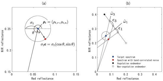
Figure 1.
Error model in the measured spectrum (a) and the errors propagated in the FVCs by algorithm-1 and -3, (b) in the red-NIR reflectance space. In (a), the blue dot indicates the target spectrum and the red dot indicates the band-correlated noise, a distance from the target spectrum. The circle around the blue dot indicates the choices of band-correlated noise. In (b), the FVCs and propagated errors for the two algorithms are indicated by empty circles on the line spanned by the vegetation and non-vegetation endmember spectra.
The errors propagated in the FVC by each of the three algorithms were derived previously []. The errors in algorithm-1 are represented in terms of the band-correlated noise and the endmember spectra (independent of the target spectrum) as
The errors propagated in the FVC by algorithm-2 are a function of the input data, expressed as
where
The errors propagated by algorithm-3 also depend on an input data set according to
where
and where
The relationship among those errors can be determined by varying the parameter θ in (Equations (7), (8), and (10)). For example, the relationship between and is shown in Figure 2 as a function of θ. In this example, the target spectrum and the vegetation and non-vegetation endmember spectra are set to (0.1,0.2), (0.05,0.4), and (0.2,0.2), respectively (Figure 2(a)). The magnitude of the input error is 0.01, and NDVI is used as the endmember model in algorithm-2. The relationship among these variables becomes an asymmetric ellipse (Figure 2(b)).
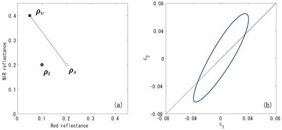
Figure 2.
An example of the relationship between , and , determined by numerical simulations. (a) shows the target spectrum (0.1,0.2), the vegetation spectrum (0.05,0.4), and the non-vegetation endmember spectrum (0.2,0.2), indicated by the blue dot, the filled and empty squares, respectively. The magnitude of the input error is set to 0.01. NDVI is used as the endmember model in algorithm-2. In (b), the ellipse is obtained by varying θ in Equations (7) and (8).
In a previous study, we derived the relationships among the errors propagated in the three FVC retrieval algorithms under a two endmember assumption []. Because the variable θ was eliminated during the derivation process, the expression describing the relationship was independent of θ. In the next subsection, we summarize the relationships among the errors associated with the three algorithms.
3.2. Relationships Among the Errors Propagated in the FVC
The relationships among the propagated errors (, , , and , the definitions of which are provided in []) were derived for all pairs. Figure 3 illustrates a schematic diagram describing the relationships among the propagated errors. The relationships are indicated by bidirectional arrows with different colors, which are labeled according to the corresponding figure numbers in the results section, discussed in detail below. The corresponding sections and equations derived in [] are also indicated in the figure. Proceeding with the explanation, we define a set S of the propagated errors according to
A pair of any two choices in S is represented by x and y. The relationship between x and y, except for the pairs and , and and , can be represented by []
where the definitions of the coefficients are summarized in []. Equation (14) represents an asymmetric ellipse, as shown in Figure 2.
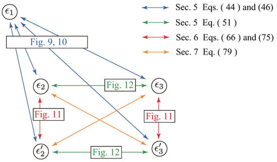
Figure 3.
Schematic diagram illustrating the relationships among the errors propagated by the FVC calculated according to each of the three algorithms. The relationships are indicated by bidirectional arrows of different colors. The figure and section numbers in the illustration indicate the results of numerical validation calculations and the derivations described in a previous study [].
The relationship between and (or between and ), denoted by a green bidirectional arrow as shown in Figure 3, becomes
where
and
Figure 4 shows a plot of Equation (15) under the same conditions (except non-vegetation endmember spectrum) as were applied in the simulation illustrated in Figure 2. Note that NDVI were chosen as the variables or constraints in both algorithms. The relationship shown in Figure 4(b) is one-to-one.
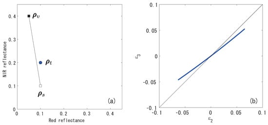
Figure 4.
Example of the relationship between and . (a) The target spectrum, vegetation spectrum, and non-vegetation endmember spectrum denoted by the blue dot, filled squares and empty squares, respectively. The values are the same as those shown in Figure 2 except non-vegetation endmember spectrum; (b) The error relationship between algorithm-2 and -3.
In general, Equation (14) describes an asymmetric ellipse rotated to a certain degree and centered at the origin (Figure 2(b)). The shape and degree of rotation (the inclination of major axis) depend on the coefficients . Similarly, the shape and rotation (or slope of the relationship) in Equation (15) depend on the coefficients .
These figures suggest an important observation: the robustness properties of the algorithms may be directly compared by deriving the rotational angle of the major axis of the ellipse. For example, if the major axis is more aligned with the X-axis than with the Y-axis (the rotational angle is less than ), the average propagated error along the X-axis exceeds that along the Y-axis. This indicates that the algorithm applied to the Y-axis is more robust than that applied to the X-axis.
4. Comparison of the Propagated Errors
An elliptical relationship is obtained by varying the angle θ of the band-correlated noise. Thus, a point on the ellipse corresponds to a certain value of θ, which is implicitly included in Equation (14). Figure 5 shows a cross plot of and for θ between 0 and . In the figure, the values of θ are indicated by the intersections with the lines of and . The red dots between and 233, and 274 and 53, indicate the range of θ in which the absolute value of is smaller than that of . This suggests that algorithm-1 is more robust under conditions in which errors are present in the target reflectance spectrum. On the other hand, the blue dots indicate the ranges in which algorithm-2 is more robust.
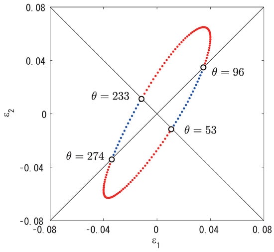
Figure 5.
Relationship between and . The segments of the ellipse, on which algorithm-1 is more robust than algorithm-2, are indicated by the red dotted lines. The values of θ are shown at the boundaries of the segments.
Note that the parameter θ depends on the type of noise present. For example, an increase in the aerosol optical thickness increases the red reflectance but decreases the NIR reflectance [], whereas the soil brightness beneath the vegetation canopy tends to shift the reflectance along the one-to-one line []. Although each effect influences the target spectrum in a different way, the robustness in the presence of noise can be compared by averaging the relative robustness over the parameter range θ. To do so, we use the slope of the major axis in the asymmetric ellipse (Equation (14)) as a robustness factor in a comparison of the two algorithms. When the slope of the major axis in the ellipse (red line in Figure 6(a)) is greater than one, the average absolute value of is less than that of . In contrast, if the slope of the ellipse is less than one (Figure 6(b)), the average absolute value of is larger than that of , indicating that algorithm-1 is less robust than algorithm-2. We next discuss a derivation of the rotation angle of the ellipse.
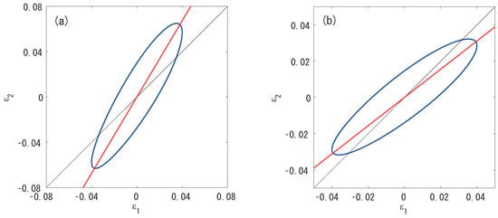
Figure 6.
Two examples of an asymmetric ellipse describing the relationship between and . In (a), the slope of the major axis exceeds unity, meaning that the average value of is less than that of . This suggests that algorithm-1 is more robust than algorithm-2 in terms of the propagated error; (b) The opposite case as is shown in (a), the conditions under which algorithm-1 is less robust than algorithm-2.
The inclination of the ellipse results from the cross terms in Equation (14). Among the cross terms, the term with coefficient provides the most significant contribution. To indicate this fact, we plot the ellipse by setting equal to zero (Figure 7(a)). As is clearly shown in the figure, the ellipse is no longer inclined. The inclination angle (illustrated in Figure 7(b)) can then be approximated by transforming (rotating) the coordinates.
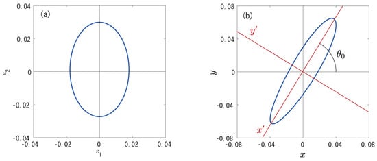
Figure 7.
Example of an asymmetric ellipse obtained by setting in Equation (14) (a), and the definitions of the angle and the new coordinate system () (b).
4.1. Derivation of the Angle
Let us define a new coordinate system obtained by rotating the original coordinate system by in the counterclockwise direction (Figure 7(b)). The geometric transformation is represented by
Substituting Equation (19) into Equation (14), we obtain the following expression for the ellipse in the new coordinate system,
where the definitions of are summarized in Appendix A.
Because the major axis is now aligned with the -axis, the coefficient of the first-order cross term, , must be close to zero,
Solving the above equation for , we obtain
Note that the coefficients, , , and depend on three factors: the target spectrum, the endmember spectra, and the choice of VI. Also, note that the term , which depends on , is negligibly small compared to the other terms []. This indicates that does not affect . Finally, the slope of the major axis is approximated by . If exceeds 1, the error propagated along the Y-axis is larger than that propagated along the X-axis.
5. Comparison between Algorithms-2 and -3 under Identical VI Conditions
The relationship between the FVC errors associated with algorithm-2 and -3, assuming identical VI, is more straightforward than the relationship described above, because the relationship is one-to-one (Equation (15)). The robustness factors may be compared using the derivative of the relationship. The derivative of with respect to is
Note that is a function of the directional parameter θ.
The robustness properties should be compared based on the average over the range of the directional parameter θ. The average derivative (represented by α) can be approximated according to the average value of ()
Applying the definition of shows that α is negligibly smaller than unity. Thus, in the context of the above equation, is considered to be
As a result, Approximation (24) becomes
Note that the average slope (α) depends on the target spectrum, endmember spectra, and choice of VI (independent of the magnitude of the input error). Also note that [] and . As a result, α becomes positive. When α is larger than one, the absolute value of is less than , meaning that algorithm-2 is more robust than algorithm-3 in terms of the propagated error in the FVC.
6. Numerical Demonstrations
The robustness factors of the LMM-based algorithms were compared for various errors in the target spectrum. Numerical simulations were conducted to compute the robustness factor ( in Equation (22) or α in Equation (26)) for various sets of endmember spectra and VI values over a range of target spectra. The coefficients in Equations (22) and (26) were determined according to three types of input data: (i) target spectrum, (ii) vegetation and non-vegetation endmember spectra, and (iii) two-band VI used in the endmember model or the constraint. The target spectra assumed in the demonstration are shown in Figure 8. For the endmember spectra, we prepared two pairs of spectra, EM1 and EM2. Although the vegetation endmembers of both pairs were identical, the spectra of the non-vegetation endmembers were different. The bright and dark soils were modeled using EM1 and EM2, respectively (Table 3). The two-band VI was selected from three VIs: NDVI, SAVI, and EVI2. The magnitude of the noise spectrum was assumed to be 0.01 throughout the demonstration (although it did not significantly influence the robustness comparisons.)
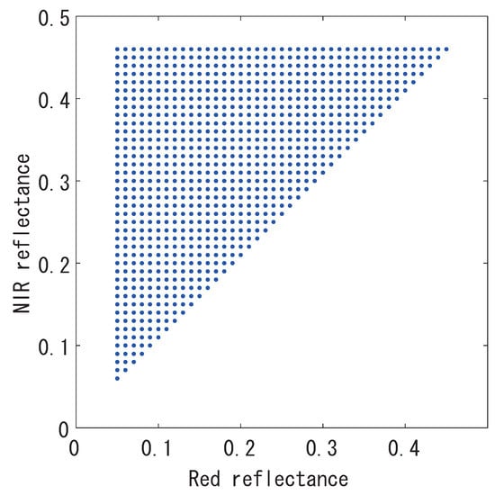
Figure 8.
Target spectra over the red-NIR reflectance space used in the numerical demonstration.

Table 3.
Two sets of endmember spectra (EM1 and EM2) used for the numerical demonstration.
The robustness factors, and α, were computed for various combinations of the input parameters. The results are summarized in four sets of figures (Figure 9, Figure 10, Figure 11, and Figure 12.) The factors are plotted as contour maps on the logarithmic scale ( or ) as a function of the red and NIR reflectance. The FVC errors propagated in the algorithms were compared, pairwise, and are indicated in the figures as “A vs. B”. In the figures, the region corresponding to positive values indicates the subspace in which the error “A” is smaller than the error “B”. Additionally, the algorithm corresponding to the error “A” is more robust than the error “B”.
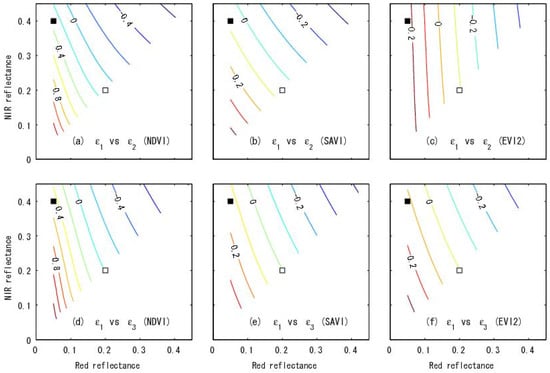
Figure 9.
Results of the numerical simulation describing the distribution of on a log scale over the red-NIR reflectance space, for comparing the performance of algorithm-1 and -2, or algorithm-1 and -3 (comparison of the inter-algorithm relationship) using EM1 as the endmember spectra. The results indicate the influences in the target spectrum and the choice of VI on . (a–c) show the -map for algorithm-1 and -2 using NDVI, SAVI, and EVI2 as the endmember models.(d–f) show the -map for algorithm-1 and -3 using those VIs as the constraints.
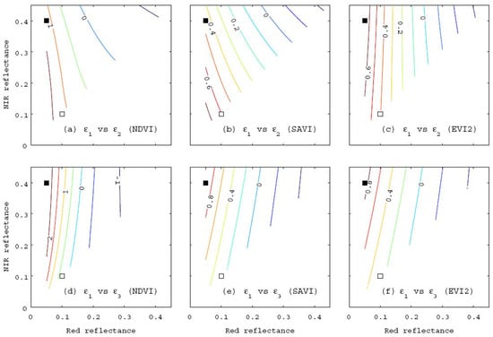
Figure 10.
Results of numerical simulations obtained by replacing the endmember spectra EM1 with EM2, shown with respect to those used in previous calculations, Figure 9. The results indicate that the relationship is influenced by the choice of VI as well as endmember spectra (non-vegetation class). A comparison with previous results is also shown. (a–c) show -map for algorithm-1 and -2 using NDVI, SAVI, and EVI2 as the endmember models. (d–f) show -map for algorithm-1 and -3 using the VIs as constraints.
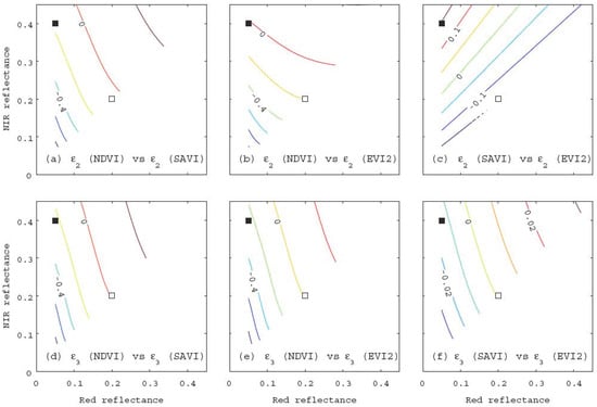
Figure 11.
Results of numerical simulations describing the distribution of on a log scale over the red-NIR reflectance spectrum. Algorithm-2 or -3 were compared using different VI conditions (comparison of the intra-algorithm relationship) and with EM1 as the endmember spectra. The results indicate the influences on the target spectrum and the choice of VI on . (a–c) show the -map for algorithm-2 using NDVI and SAVI, NDVI and EVI2, and SAVI and EVI2 as the endmember models. (d–f) show -map for algorithm-3 using the same sets of VI used in the upper three panels as constraints.
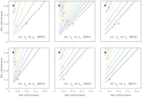
Figure 12.
Results of numerical simulations describing a distribution of α on a log scale over the red-NIR reflectance spectrum to compare algorithm-2 and -3 using identical VI conditions (comparison of the inter-algorithm relationship). The results indicate the influence of the target spectrum, endmember spectra, and choice of VI on . (a–c) show the -map using NDVI and SAVI, NDVI and EVI2, and SAVI and EVI2 as the conditions for algorithm-2 and -3 based on EM1. (d–f) show the -map for the VIs assumed in the upper three panels, based on EM2.
Figure 9 compares algorithm-1 and -2 (upper three panels), and algorithm-1 and -3 (lower three panels) for the endmember pair EM1 with the three VIs. In general, is independent of the target spectrum. Therefore, variations in are caused by the variations in . In the figures, the contour lines for are proximal to the lines spanned by the two-endmember spectra. This suggests that, for the target spectra located on the left-hand sides of the lines spanned by the endmember spectra, algorithm-1 is more robust than the other two algorithms.
Figure 10 shows a comparison similar to that shown in Figure 9, with different endmember spectra, EM2. Recall that EM2 is a darker non-vegetation endmember spectrum than EM1. In the figures, the positive value regions increased in size (relative to the regions in the previous figures), indicating that algorithm-1 is more robust than the other two algorithms over a wider range of the target spectra. This also indicates that algorithm-1 is more robust than the others for darker non-vegetation spectra.
In summary, algorithm robustness depends on the endmember spectra assumed in the algorithm. Even when assuming identical endmember spectra, the robustness properties of two algorithms can vary with the measured target spectrum. In general, the brightness of the target spectrum and the position of its reflectance spectra relative to the endmember spectra are important factors.
Figure 11 shows an intra-algorithm comparison (for different VIs) of algorithm-2 and -3 using EM1. Although the contour lines showed similar patterns, the use of SAVI or EVI2 for (upper-right figure) resulted in different patterns, and the mechanism remains unclear. The line spanned by the endmember spectra was no longer the discriminator of robustness in this case.
Figure 12 plots the values of α to compare algorithm-2 and -3 for a given VI with two sets of endmember spectra. The upper three panels show the results using EM1, and the lower three panels present results using EM2. In general, when the VI of the target spectrum is high, algorithm-2 is more robust (hence, a better choice) to noise in the target reflectance spectrum. Interestingly, the contour patterns were similar, and were comparable to the pattern considered to be an exception, as shown in Figure 11 (upper right panel). We also note that the differences in the non-vegetation spectra did not significantly influence the patterns of the contour lines, whereas the magnitude of α varied significantly.
7. Conclusions
This study derived the robustness factors necessary for comparing LMM-based FVC algorithms. The derivations relied on analytical expressions for the relationships between the errors propagated in FVC, introduced previously []. Based on our derivations, the relative robustness between the two algorithms can be judged by a single factor, (or α). This approach is significant in that the robustness of different algorithms can be compared deterministically (statistical approaches are not necessary) using only prior knowledge of a target field and the endmember spectra assumed in the algorithms. Also note that parameter studies and iterative approaches are not involved in comparison processes. These factors provide important information for discussions of the optimum algorithm under two-endmember and two-band assumptions.
Although the range of practical applications to which the results of this study may be applied is somewhat limited due to the assumptions made on the LMM (number of bands and endmember species), the findings and the essence of the theoretical development contribute to a better understanding of the FVC retrieval algorithms in terms of robustness to noise. Further studies are required to expand the techniques to achieve broader applicability.
Acknowledgements
This work was supported by the Circle for the Promotion of Science and Engineering (KO) and JSPS KAKENHI 21510019 (HY).
Appendix
Coefficients in the geometric transform equation.
References
- Myneni, R.B.; Maggion, S.; Iaquinta, J.; Privette, J.L.; Gobron, N.; Pinty, B.; Kimes, D.S.; Verstreate, M.M.; Williams, D.L. Optical remote sensing of vegetation: Modeling, caveats, and algorithms. Remote Sens. Environ. 1995, 51, 169–188. [Google Scholar] [CrossRef]
- Hall, F.G.; Townshend, J.R.; Engman, E.T. Status of remote sensing algorithms for estimation of land surface state parameters. Remote Sens. Environ. 1995, 51, 138–156. [Google Scholar] [CrossRef]
- Wang, C.; Qi, J.; Cochrane, M. Assessment of Tropical Forest Degradation with Canopy Fractional Cover from Landsat ETM+ and IKONOS Imagery. Earth Interact. 2005, 9, 1–18. [Google Scholar] [CrossRef]
- Carlson, T.N.; Arthur, S.T. The impact of land use-land cover changes due to urbanization on surface microclimate and hydrology: A satellite perspective. Global Planet Change 2000, 25, 49–65. [Google Scholar] [CrossRef]
- Lobell, D.B.; Asner, G.P.; Law, B.E.; Treuhaft, R.N. Subpixel canopy cover estimation of coniferous forests in Oregon using SWIR imaging spectrometry. J. Geophys. Res. 2001, 106, 5151–5160. [Google Scholar] [CrossRef]
- Barlage, M.; Zeng, X. The Effects of observed fractional vegetation cover on the land surface climatology of the community land model. J. Hydrometeorol. 2004, 5, 823–830. [Google Scholar] [CrossRef]
- Zhang, J.; Walsh, J.E. Thermodynamic and hydrological impacts of increasing greenness in northern high latitudes. J. Hydrometeorol. 2006, 7, 1147–1163. [Google Scholar] [CrossRef]
- Foody, G.M.; Cox, D.P. Sub-pixel land cover composition estimation using a linear mixture model and fuzzy membership functions. Int. J. Remote Sens. 1994, 15, 619–631. [Google Scholar] [CrossRef]
- Wittich, K.P.; Hausing, O. Area-averaged vegetative cover fraction estimated from satellite data. Int. J. Biometeorol. 1995, 38, 209–215. [Google Scholar] [CrossRef]
- Small, C. Estimation of urban vegetation abundance by spectral mixture analysis. Int. J. Remote Sens. 2001, 22, 1305–1334. [Google Scholar] [CrossRef]
- Bateson, C.A.; Asner, G.P.; Wessman, C.A. Endmember bundles: A new approach to incorporating endmember variability into spectral mixture analysis. IEEE Trans. Geosci. Remote Sens. 2000, 38, 1083–1094. [Google Scholar] [CrossRef]
- Xiao, J.; Moody, A. A comparison of methods for estimating fractional green vegetation cover within a desert-to-upland transition zone in central New Mexico, USA. Remote Sens. Environ. 2005, 98, 237–250. [Google Scholar] [CrossRef]
- Van de Voorde, T.; Vlaeminck, J.; Canters, F. Comparing different approaches for mapping urban vegetation cover from landsat ETM+ data: A case study on Brussels. Sensors 2008, 8, 3880–3902. [Google Scholar] [CrossRef] [PubMed]
- Horwitz, H.M.; Nalepka, R.F.; Hyde, P.D.; Morgenstern, J.P. Estimating the Proportions of Objects Within a Single Resolution Element of a Multispectral Scanner; Technical Report NASA Contract NAS-9-9784; University Michigan: Ann Arbor, MI, USA, 1971. [Google Scholar]
- Settle, J.J.; Drake, N.A. Linear mixing and the estimation of ground cover proportions. Int. J. Remote Sens. 1993, 14, 1159–1177. [Google Scholar] [CrossRef]
- Ichoku, C.; Karnieli, A. A review of mixture modeling techniques for sub-pixel land cover estimation. Rmote Sens. Rev. 1996, 13, 161–186. [Google Scholar] [CrossRef]
- Smith, M.O.; Johnson, P.E.; Adams, J.B. Quantitative determination of mineral types and abundances from reflectance spectra using principal components analysis. J. Geophys. Res., Suppl. 1985, 90, C797–C804. [Google Scholar] [CrossRef]
- Adams, J.B.; Smith, M.O.; Johnson, P.E. Spectral mixture modeling: A new analysis of rock and soil types at the Viking Lander 1 site. J. Geophys. Res. 1986, 91, 8098–8112. [Google Scholar] [CrossRef]
- Chang, C.I.; Zhao, X.L.; Althouse, M.; Pan, J.J. Least squares subspace projection approach to mixed pixel classification for hyperspectral images. IEEE Trans. Geosci. Remote Sens. 1998, 36, 898–912. [Google Scholar] [CrossRef]
- Cochrane, M.A.; Souza, C.M. Linear mixture model classification of burned forests in the Eastern Amazon. Int. J. Remote Sens. 1998, 19, 3433–3440. [Google Scholar] [CrossRef]
- Gillespie, A.R. Spectral mixture analysis of multispectral thermal infrared images. Remote Sens. Environ. 1992, 42, 137–145. [Google Scholar] [CrossRef]
- Smith, M.O.; Ustin, S.L.; Adams, J.B.; Gillespie, A.R. Vegetation in deserts: I. A regional measure of abundance from multispectral images. Remote Sens. Environ. 1990, 31, 1–26. [Google Scholar] [CrossRef]
- Jasinski, M.F. Estimation of subpixel vegetation density of natural regions using satellite multispectral imagery. IEEE Trans. Geosci. Remote Sens. 1996, 34, 804–813. [Google Scholar] [CrossRef]
- Kallel, A.; Héarat-Mascle, S.L.; Ottlé, C.; Hubert-Moy, L. Determination of vegetation cover fraction by inversion of a four-parameter model based on isoline parametrization. Remote Sens. Environ. 2007, 111, 553–566. [Google Scholar] [CrossRef]
- Carpenter, G.A.; Gopal, S.; Macomber, S.; Martens, S.; Woodcock, C.E. A neural network method for mixture estimation for vegetation mapping. Remote Sens. Environ. 1999, 70, 138–152. [Google Scholar] [CrossRef]
- Guilfoyle, K.J.; Althouse, M.L.; Chang, C.-I. A quantitative and comparative analysis of linear and nonlinear spectral mixture models using radial basis function neural networks. IEEE Trans. Geosci. Remote Sens. 2001, 39, 2314–2318. [Google Scholar] [CrossRef]
- Jimenéz-Muñoz, J.C.; Sobrino, J.A.; Plaza, A.; Guanter, L.; Moreno, J.; Martinez, P. Comparison between fractional vegetation cover retrievals from vegetation indices and spectral mixture analysis: Case study of PROBA/CHRIS data over an agricultural area. Sensors 2009, 9, 768–793. [Google Scholar] [CrossRef] [PubMed]
- Obata, K.; Yoshioka, H. Inter-algorithm relationships for the estimation of the fraction of vegetation cover based on a two endmember linear mixture model with the VI constraint. Remote Sens. 2010, 2, 1680–1701. [Google Scholar] [CrossRef]
- Obata, K.; Yoshioka, H. Relationships between errors propagated in fraction of vegetation cover by algorithms based on a two-endmember linear mixture model. Remote Sens. 2010, 2, 2680–2699. [Google Scholar] [CrossRef]
- Goward, S.N.; Markham, B.; Dye, D.G.; Dulaney, W.; Yang, J. Normalized difference vegetation index measurements from the advanced very high resolution radiometer. Remote Sens. Environ. 1991, 35, 257–277. [Google Scholar] [CrossRef]
- Miura, T.; Huete, A.; Yoshioka, H. Evaluation of sensor calibration uncertainties on vegetation indices for MODIS. IEEE Trans. Geosci. Remote Sens. 2000, 38, 1399–1409. [Google Scholar] [CrossRef]
- Gong, P.; Zhang, A. Noise effect on linear spectral unmixing. Ann. GIS 1999, 5, 52–57. [Google Scholar] [CrossRef]
- Barducci, A.; Mecocci, A. Theoretical and experimental assessment of noise effects on least-squares spectral unmixing of hyperspectral images. Opt. Eng. 2005, 44, 087008. [Google Scholar]
- Soffer, R.J.; Neville, R.A.; Staenz, K.; White, H.P. Sensitivity of Spectral Unmixing Analysis to a Spectrally Dependent Gain Error in Hyperspectral Data. In Proceedings of the IEEE International Conference on Geoscience and Remote Sensing Symposium, IGARSS 2006, Denver, CO, USA, 31 July–4 August 2006; pp. 1130–1133.
- Shimabukuro, Y.E.; Smith, J.A. The least-squares mixing models to generate fraction images derived from remote sensing multispectral data. IEEE Trans. Geosci. Remote Sens. 1991, 29, 16–20. [Google Scholar] [CrossRef]
- Gutman, G.; Ignatov, A. The derivation of the green vegetation fraction from NOAA/AVHRR data for use in numerical weather prediction models. Int. J. Remote Sens. 1998, 19, 1533–1543. [Google Scholar] [CrossRef]
- Rouse, J.W.; Haas, R.H.; Schell, J.A.; Deering, D.W. Monitoring Vegetation Systems in the Great Plains with ERTS. In Proceedings of the Third Earth Resources Technology Satellite-1 Symposium, Washington, DC, USA, 1974; pp. 309–317.
- Huete, A.R. A soil-adjusted vegetation index (SAVI). Remote Sens. Environ. 1988, 25, 295–309. [Google Scholar] [CrossRef]
- Jiang, Z.; Huete, A.R.; Didan, K.; Miura, T. Development of a two-band enhanced vegetation index without a blue band. Remote Sens. Environ. 2008, 112, 3833–3845. [Google Scholar] [CrossRef]
- Zeng, X.; Dickinson, R.E.; Walker, A.; Shaikh, M.; Defries, R.S.; Qi, J. Derivation and evaluation of global 1-km fractional vegetation cover data for land modeling. J. Appl. Meteorol. 2000, 39, 826–839. [Google Scholar] [CrossRef]
- Holben, B.N. Characteristics of maximum-value composite images from temporal AVHRR data. Int. J. Remote Sens. 1986, 7, 1417–1434. [Google Scholar] [CrossRef]
- Yoshioka, H.; Huete, A.; Miura, T. Derivation of vegetation isoline equations in red-NIR reflectance space. IEEE Trans. Geosci. Remote Sens. 2000, 38, 838–848. [Google Scholar] [CrossRef]
© 2011 by the authors; licensee MDPI, Basel, Switzerland. This article is an open access article distributed under the terms and conditions of the Creative Commons Attribution license (http://creativecommons.org/licenses/by/3.0/).