A New Window-Based Program for Quality Control of GPS Sensing Data

1
Department of Civil, Architectural & Environmental Engineering, Sungkyunkwan University, Suwon 440-746, Korea
2
Department of Spatial Information Engineering, Pukyong National University, Busan 608-737, Korea
*
Authors to whom correspondence should be addressed.
Remote Sens. 2012, 4(10), 3168-3183; https://doi.org/10.3390/rs4103168
Submission received: 23 August 2012
/
Revised: 16 October 2012
/
Accepted: 16 October 2012
/
Published: 18 October 2012
Abstract
:The main purpose of this study is to develop a new Windows-based program that calculates a quality control parameter that shows the quality of Global Positioning System (GPS) observations using GPS data in a Receiver INdependent Exchange (RINEX) format. This new program, Global Positioning System Quality Control (GPSQC), allows general GPS users to easily and intuitively check the quality of GPS observations before post-processing, which will lead to the improvement of GPS positioning precision in diverse areas of GPS applications. The GPSQC is designed to control the multi-path, cycle slip, and ionospheric errors of L1 and L2 signals in GPS observations. The GPSQC was developed using C#.NET language for the Window series with Microsoft Graphical User Interfaces (MS GUIs). This program gives brief information for GPS observations, time series plots, graphs of quality control parameters, and a summary report in MS word, Excel and PDF formats. It can simply perform quality checking of GPS observations that is difficult for surveyors conducting field work. We expect that GPSQC can be used to improve the accuracy of positioning and to solve time-consuming problems due to data loss and large errors in GPS observations.
1. Introduction
The quality of GPS positioning is related to a number of error factors [1]. To obtain high-precision positioning results, we need to identify the main error sources impacting the quality of GPS sensing data (i.e., GPS observations). In GPS data processing, multi-path, cycle slips, atmospheric delays and quasi-random errors are the main sources that can deteriorate the quality of the observations and subsequently, the quality of positioning results [1,2].
To obtain consistent high-precision positioning results with the GPS carrier-phase analysis, errors that are not specified in a functional or stochastic model must be detected correctly, removed and controlled in data processing. Reliability, which refers to the ability to detect such errors and to estimate the effects that they may have on a solution, is one of the main issues in GPS data quality control. A comprehensive investigation of quality issues in GPS observations was performed by the Special Study Group (SSG) 1.154 of the International Association of Geodesy (IAG) between 1996 and 1999 [3] and by the University NAVSTAR Consortium (UNAVCO).
Two quality control programs, Translation, Editing and Quality Checking (TEQC) and GPS Qualtiy Control (GQC), are now available for GPS observations. The conceptual and theoretical background of TEQC was originally written by Chris Rocken [4] at UNAVCO and has been extensively modified by Teresa Van Hove, John Braun and James Johnson [5]. Subsequently, a software-toolkit called TEQC was developed by Louis Estey and Charles Meertens [5] to treat mixed satellite constellations, such as GPS, GLObal NAvigation Satellite System (GLONASS) and Satellite Based Augmentation System (SBAS). TEQC allows the user to translate the GPS data from a binary format to an ASCII format called the Receiver INdependent Exchange (RINEX) format, which allows for format modifications and quality control of the GPS observations before analysis of the GPS data. TEQC is 100% noninteractive to assist its use with automatically executed scripts, and has a command line interface modeled after common UNIX commands. TEQC has been tested on 32-bit processors with math coprocessors from a 486/DX up to a P4 running Windows 95/98/NT/2000/XP with DOS emulation windows [5].
GQC was developed as part of a Ph.D. dissertation [6] in GPS geodesy at the Department of Geomatics, University of Melbourne. GQC was originally called Quimby, but was substantially re-written and re-packaged to have more functionality. GQC provides preliminary quality and data integrity of dual frequency GPS observations in RINEX format. It is able to process individual RINEX files or automatically process files being created by a network of GPS base stations. GQC was written for use with the Microsoft Windows family of operating systems. It will run on all 32 bit Windows operating systems (Win9x, ME, XP, NT and 2000).
However, neither of these programs is user-friendly because TEQC and GQC executables are not available on MS Windows GUIs; they are all command line programs. Therefore, the quality control results of GPS observations provided by TEQC and GQC are not easily understood by general GPS users, other than experts, and, in the general, non-academic parts of GPS applications, the data quality check with these programs are often ignored or omitted. Accordingly, the desired precision level is not achieved even though the GPS sensing data observed from field work are post-processed precisely. In this case, GPS observations must be repeated until the desired precision level is achieved. This process is significantly time-consuming and costly.
The main purpose of this study is to develop a Windows-based program that calculates the quality control parameter that shows the quality of GPS observations using the GPS sensing data in a RINEX format. This allows general GPS users to easily and intuitively check the quality of GPS observations before post-processing, which will lead to the improvement of GPS positioning precision in diverse areas of GPS applications. In addition, by directly determining the observation adequacy and re-observation simultaneously during observation, the expense in terms of time and cost due to the reduced precision in the GPS post-processing can be minimized.
In this paper, we describe GPSQC, a Windows-based quality control program that gives the variety of information to judge the suitability of GPS observations within the observation time in the field and enhances the precision of data processing. The GPSQC program was designed to directly calculate the geometric distribution, multi-path effect, ionospheric delay and cycle slip effect from observation and navigation files at a single point. This program checks the observation data from a single station and is available to run on MS Windows operating systems with GUIs (Window 9x, 2000, XP and higher). The quality of data from any GPS receiver can be checked if the observation data are in the RINEX format. If satellite position information is to be calculated and used by GPSQC, then a RINEX navigation file must also be used. RINEX translators developed at the University of Bern [7] are publicly available. In addition, batch and script files translate raw data to a RINEX format, process the data with GPSQC, then display the output plot files using a graphical display from a single command line. Batched runs can generate hard copies of the quality control summary and graphics files.
2. Quality Control Algorithms for GPS Observations
GPSQC consists of five data quality/availability parts: geometric distribution (sky plot, satellite elevation, azimuth), dilution of precision (DOP), multi-path (MP1, MP2) of L1 and L2, ionospheric delays (I1, I2) of L1 and L2, and cycle slip effects (cyc) of phase observations. The fundamental algorithms adopted in GPSQC follow the same algorithms used in the TEQC program. GPSQC uses the cycle slip algorithm developed by Blewitt [8] and the multi-path estimation equations in [5].
2.1. Satellite Elevation and Dilution of Precision (DOP)
GPS errors are mainly affected by satellite arrangements [9]. It is possible to identify these arrangements by calculating the azimuth and altitude of all of the satellites during the periods of observations. The observables of the 3-D geodetic model are the azimuth (α), the vertical angle (β) and the slant distance (s).
The forces of gravitational and non-gravitational origin perturb the motion of GPS satellites, causing the orbits to deviate from a Keplerian ellipse in inertial space defined by the six elements, semi-major axis a, eccentricity e, inclination i, longitude of the ascending node Ω, angle of perigee ω, and true anomaly f or eccentric anomaly E. The perturbations are characterized by periodic and secular components, and must be continually determined through the analysis of tracking data. In order to adequately describe the GPS orbits for the interval of time during which the ephemeris information is transmitted, a representation based on Keplerian elements plus perturbations is used. The satellite ephemerides are broadcasted two hours in advance of the epoch for which they were calculated. Generally, the update occurs daily, though is sometimes more frequent. Therefore, the portions of ephemeris data for the second through fourteenth days are not normally transmitted, except when the upload is not possible. At the same time, each satellite’s clock state is estimated and then extrapolated into the future, and the information is finally formatted into the navigation message. It is easy to calculate the earth-centered and earth-fixed (ECEF) Cartesian coordinates of a satellite (XS, YS, ZS) on a specific epoch using satellite ephemeris information and WGS84 constants.
The α and β between the satellite and receiver were derived from Equations (1) and (2), respectively. The ECEF Cartesian coordinate of the receiver was calculated from the approximate coordinate recorded in a header part of the GPS observation data. The earth-fixed reference system is presently based on the WGS84 system [9],
where, φR and λR are the geodetic coordinates of the receiver based on the WGS84 ellipsoid, which is calculated by the direct coordinate conversion from ECEF to geodetic [10]. This conversion is not exact and provides centimeter accuracy for heights below 1,000 km. ΔX, ΔY and ΔZ are the geometrical differences in the ECEF coordinate system between the receiver (XR, YR, ZR) and GPS satellite (XS, YS, ZS).
Dilution of precision (DOP) values are commonly used to indicate the quality of satellite arrangements. DOP is the ratio of positioning accuracy to the observation accuracy. DOP is always a number greater than unity when there are no redundant observations. The DOP values vary from epoch to epoch according to the change of a satellite’s geometric distribution. The satellite’s geometric distribution does not cause inaccuracies in the position determination that can be measured in meters. In fact, the DOP values amplify other inaccuracies. High DOP values merely amplify other GPS errors to a greater extent than do low DOP values. A number of different DOP factors are possible, depending on the coordinate component, or combination of coordinate components of the local geodetic coordinate system, usually expressed as N, E and H. Several DOP factors are calculated as follows [11].
where σ is usually taken to be equal to the total user equivalent range error,
,
,
and
are the corresponding variances of position in northing N, easting E, height H and time T on the local geodetic coordinate system, respectively [11].
The case of GPS point positioning, which requires the estimation of four parameters (3-D position and receiver clock error), the most appropriate DOP factor is the GDOP. GDOP can be interpreted as the reciprocal of the volume of a tetrahedron that is formed from four satellites and the receiver positions. Hence, the best geometric situation for point positioning is when the volume is a maximum, which therefore requires GDOP to be a minimum. Generally, if the GDOP rises above 6, the satellite geometry is not desirable [12].
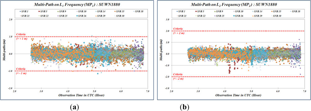
2.2. Multi-Path Effects
Multi-paths are radio signals whereby a GPS signal is reflected off some object reaching the GPS receiver’s antenna. These signals take longer to reach the receiver than if they had travelled along a direct path. As a result, multiple copies of the transmitted signal are present in the tracking loop of the receiver [9]. This can result in the GPS miscalculating its position because the signals may have traveled from centimeters to meters further to reach their targets than a direct line-of-sight signal path would have travelled.
Multi-paths affect not only the code range and carrier-phase measurements but also the measured signal power, which is an average of the composite signal power due to the direct and reflected signal carrier. Although the multi-path effect can be reduced by choosing sites without multi-path reflectors or by using choke-ring antennas to mitigate the reflected signal, it is difficult to eliminate all multi-path effects from GPS observations. Further, multi-path errors are also unique for each receiver and are uncorrelated between signals. Some unmodeled biases remain in GPS observations, even after such data differencing. Therefore, multi-path effects are very difficult to calculate. Multi-path effects are a major residual error source in the double-differenced GPS observables, and they can have a significant impact on the positioning results. If we know the magnitude of multi-path effects, then it will be possible to carry the quality control of GPS observations.
The magnitude of multi-path effect is defined as the ranging error caused by the reflected carrier-phase GPS signal. The multi-path effects on the pseudo-range observables of L1 and L2 frequencies (MP1 and MP2, respectively) can be written as linear combinations as follows.
where P1 and P2 are L1 and L2 pseudo-range (m), Φ1 and Φ2 are L1 and L2 phase measurement (m), α = (f1/f2)2 and f1 and f2 are L1 and L2 phase frequencies (Hz), respectively.
Multi-path analysis creates numerical summaries and graphical displays of pseudo-range multi-path effects for both single and dual frequency data.
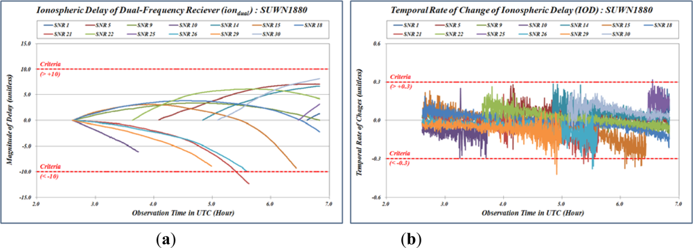
2.3. Ionospheric Effects
The delay of GPS signals occurs through the ionosphere, which is a shell of electrons and electrically charged atoms and molecules that surrounds the earth, stretching from a height of approximately 50 km to more than 1,000 km. Ionospheric delay is one of the largest sources of error in GPS positioning and navigation and it can vary from a few meters to more than twenty meters within one day [13]. The delay is proportional to the number of electrons and is inversely proportional to f2. Thus, the effect is dispersive, and depends on the frequency f. If the delay was not accounted for, the range errors on the L1 frequency in the zenith direction could reach 30 m [14].
The magnitude of ionospheric range errors is related to the Total Electron Content (TEC) along the signal path from a GPS satellite to the receiver and is dependent on the signal frequency and the level of ionospheric activity. The TEC is defined as the total number of electrons that are contained in a vertical column with a cross-sectional area of 1 m2 along the signal path between the satellite and the receiver.
GPS users with dual-frequency P-code receivers can correct the ionospheric range error through an appropriate combination of the pseudo-ranges observed on L1 and L2. Single-frequency users with C/A-code receivers do not have that correction. They either have to persevere with the reduced measurement accuracy or employ a model for the correction of ionospheric range errors.
Several electron density models such as Bent [15] and International Reference Ionosphere (IRI) [16] are available for the study of electron density profiles at different altitudes from the ionosphere [17,18]. The Klobuchar model [19] is the only model available for estimating the ionospheric time delay for single frequency GPS users.
The Klobuchar model is a simple computational model with an ideal description for the ionosphere’s average behavior. In dual frequency receivers, the ionospheric delay can be estimated precisely by taking advantage of the dispersive nature of the ionosphere. The delay is estimated by measuring the difference in arrival times of the two GPS frequencies.
In this study, we calculated the ionospheric delay (iondual) of dual-frequency receiving data using carrier-phase observations in L1 and L2. We also used the broadcast message containing the ionospheric model coefficients for computing the ionospheric group delay along the signal path to obtain a single-frequency delay in the ionosphere (ionL1, ionL2).
The ionospheric delay (iondual) at one epoch using a dual frequency receiver is
where N2 and N1 are L1 and L2 carrier-phase ambiguity, respectively.
Because we are only interested in changes of iondual over time for the individual PRN (Pseudo Random Noise), Equation (10) can be written as follows;
Additionally, the ionospheric delay (ionL1, ionL2) for a single frequency receiver is calculated with an algorithm developed by Klobuchar [19]. The ionospheric delay of L1 frequency can be computed by the Klobuchar model using the eight ionospheric model coefficient in the navigation file and quality control parameters (α, β, φR and λR).
The Klobuchar algorithm is based on the shell model or single layer model of the ionosphere. The implicit assumption is that the TEC is concentrated in an infinitesimally thin spherical layer at a certain height, e.g., 350 km [9]. The algorithm is known to be compensated for 50∼60% of the actual group delay.
The ionospheric delay of L1 frequency (ionL1) is
where the factor F is a mapping function that converts the vertical ionospheric delay at the ionospheric pierce point to the slant delay at the receiver point. The ionospheric pierce point is the intersection of the line of sight and the ionospheric layer. All abbreviations used in Equation (12) are shown in Table 1, which refers to the broadcast ionospheric model suggested by Lieck [9].
The relationship between the time delays on the two frequencies f1 and f2 due to the ionosphere is
hence, the L2 ionospheric effect is approximately 1.6469 times that of L1 (1.6469 ≈ f12/f22). Therefore, L2 ionospheric delay (ionL2) can be expressed as
The temporal rate of change of the ionospheric delay is used to monitor epoch to epoch in order to detect large change in phase ambiguities; that is, any slips in tracking of L1 and/or L2. A minimum amount of variability must be assumed because the paths of the signals from the current epoch to the next epoch have changed due to the path change in the ionosphere, the time variation of the ionosphere, the motion of the satellite and the possible motion of antenna itself [5].
The temporal rate of change as the time derivative of the ionospheric delay (iod) at the specific epoch tdata is as follows [5];
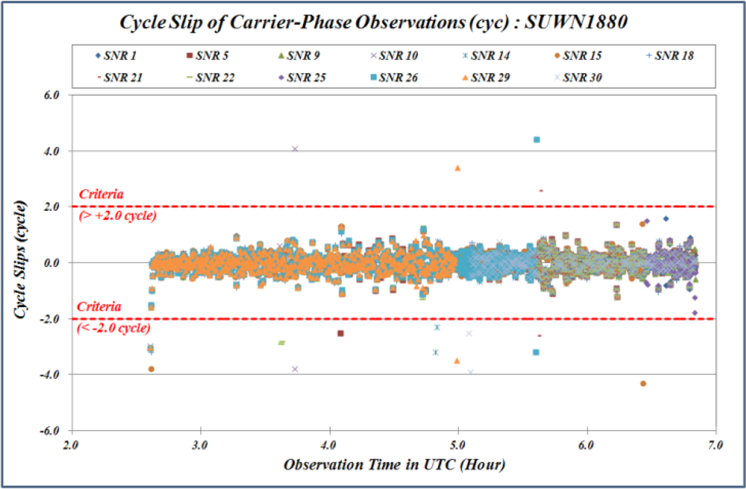
2.4. Cycle Slip Effects
Cycle slip is an error resulting from the instantaneous loss of carrier-phases in GPS observations. Cycle slip is associated with a failure of the carrier-phase tracking loop either because the signal is blocked physically or because the signal is weak [9]. The detection of cycle slip is important for precise geodetic positioning using carrier-phase data. Geodetic quality receivers usually flag the user when a cycle slip has occurred. To repair the cycle slip in GPS observations, the exact characteristics of cycle slips need to be known.
A cycle slip can be detected if double and triple differences are formed using more than two points in GPS carrier-phase observations, which are observed simultaneously. In the case of a single GPS observation, however, a different methods for cycle slip detection based on undifferenced carrier-phase observations should be applied. In this study, cycle slip detection is performed using the TurboEdit algorithm developed by Blewitt [8]. TurboEdit is an algorithm for cycle slip identification and repair as well as outlier removal using undifferenced, dual-frequency GPS observation at single point. In this algorithm, the detection of cycle slip is based on Melbourne-Wübenna (M-W) linear combination [20] and a geometry-free combination.
The M-W linear combination has been widely applied to cycle slip detection in undifferenced observation and double differences. A major advantage of M-W combination is that it is not only geometry-free but also ionospheric-free. Therefore, it can be used even if the GPS receiver undergoes high levels of dynamics and/or ionospheric variation. For ionospheric combinations, the M-W combination was used in the TurboEdit algorithm to detect and repair cycle slip. The M-W combination uses pseudo-range observations that have greater noise than carrier-phase observations. Under some observation conditions, the pseudo-range noise may be much larger than usual, for example, in the presence of multi-path, increased ionospheric delay, and low DOP. In such circumstances, the recursive averaging algorithm used in TurboEdit may fail to detect small cycle slips of 1–2 cycles [20].
For observations from a dual-frequency GPS receiver, the M-W combination can be expressed as follows,
where λMW = c/(f1 − f2) ≈ 0.86 m and NMW = N1 − N2 are the wide-lane wavelength and wide-lane ambiguity, respectively.
The wide-lane ambiguity can be easily obtained from Equation (16) as follows,
As long as the phase observations are free of cycle slips, the wide-lane ambiguity remains quite stable over time. In utilizing the M-W combination to detect cycle slips, a recursive averaging filter is used in TurboEdit as follows,
where N̄WL is the mean value of NWL, k and k − 1 represent the current and previous observation epochs, respectively. The standard deviation of N̄WL at epoch (k) is σ(k). When the following conditions are satisfied, it is considered that a cycle slip (cyc) occurs,
and
where σ(k) was considered as configuration parameter and set at 0.5 cycles as a default value.
3. Development of the GPSQC Program
GPSQC was developed using C#.NET language, which is based on MS Windows GUIs. This program gives the user brief information about GPS observations, time series plots and graphs of quality control parameters. It checks the observation and navigation files from a single station and is available to run on a Windows operating system (Windows 9x, 2000, XP and higher) which is widely used in the multi-tasking environment for PCs. The user interface is relatively easy, as it is based on the Windows series. The fundamental input required by GPSQC is the RINEX Version 2.0 or higher observation and navigation files that contain only GPS data. A RINEX format translator that translates raw data to a RINEX format is publicly available and was developed at the University of Bern.
The program forms linear combinations of the GPS range and carrier-phase data to compute the following: (1) the L1 pseudo-range multi-path for C/A- or P-code observations, (2) the L2 pseudo-range multi-path for P-code observations, (3) the ionospheric phase effects on the L1 carrier frequency, and (4) the rate of change of the ionospheric delay. The program also writes data summary files with information about the GPS observations, geometric distribution (DOPs, elevation and azimuth) and cycle slips effects, etc.. The quality control process is completely automated by GPSQC and the resulting report can be used to evaluate the observation data prior to GPS data processing.
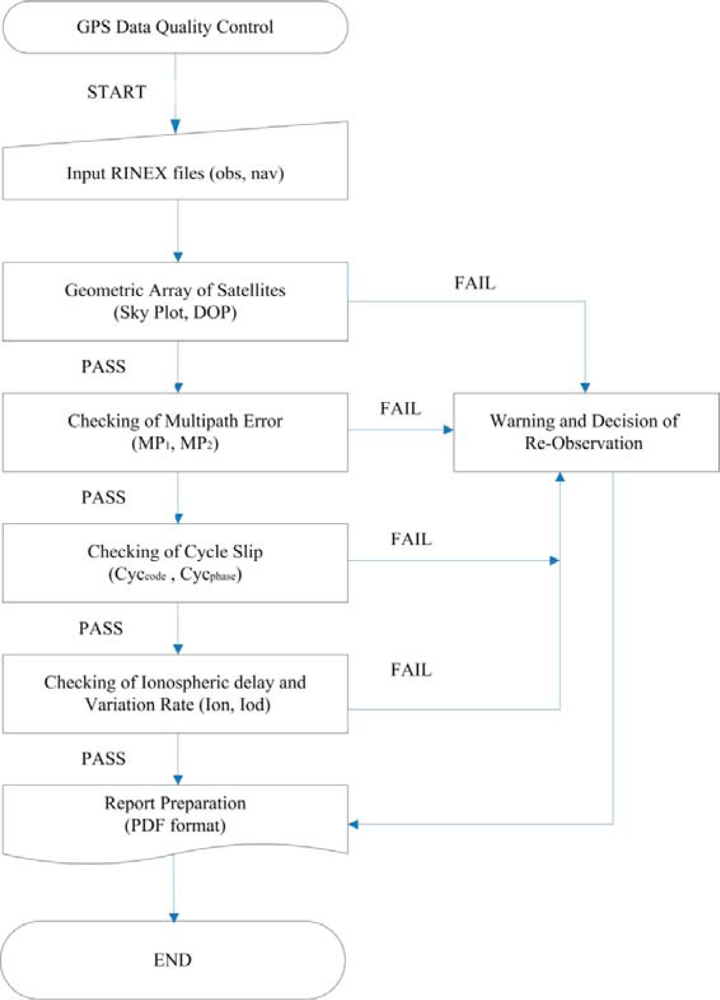
Figure 1 shows the general flow of the GPSQC program. The GPSQC can be performed to compare the calculated quality control parameters with the specified criteria and give the percentage (%) of data per criterion. This program requires certain criteria before processing. The values of these criteria can influence the results obtained. It is important to detail the three criteria (a ∼ c) as follows:
- Elevation cut-off angle: 15 degrees
- Minimum gap in data to be detected: 2 min
- Maximum L2-Ionospheric time-rate of change: 800 cm/h (or approximately 0.22 cm/s)
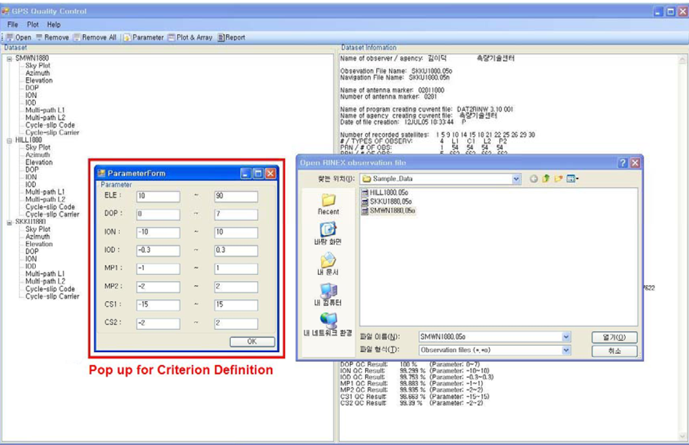
Figure 2 shows the interactive Window of the GPSQC program. By selecting “Open File” in the main menu with the mouse button, two RINEX formatted files, observation and navigation files can be chosen from a specified directory. Selecting the QC button or processing icon, GPSQC calculates the eight QC parameters. To following procedure is used to process an individual RINEX file.
- Step 1. Load GPSQC.
- Step 2. Select File/Open using the icon on the toolbar.
- Step 3. Navigate to the folder containing the files.
- Step 4. Select “Observation Files, *.obs” and “Navigation Files, *.nav”.
- Step 5. Define the criterion (see the red box in Figure 2).
- Step 6. Select the ‘Processing’ icon on the toolbar.
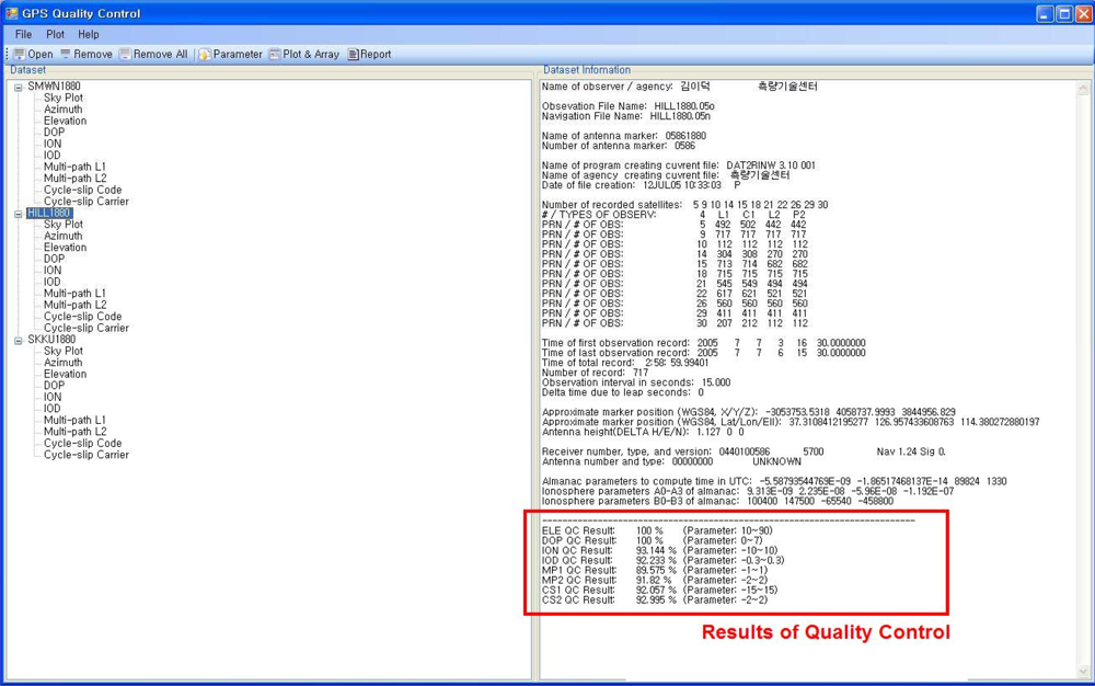
GPSQC will then begin processing. When the processing is complete, the status bar at the bottom of one window will indicate ‘Ready’ and the output will be displayed in another window. The progress bar on the bottom right of the window indicates the amount of time it will take to finish data processing. Graphs and time series of quality control indicators, provided so that the user can easily understand the result of quality control will be displayed in the processing window when the processing is complete.
The report file can be generated automatically by turning on the selective graphing format option for PDF, MS word and Excel formats. Graphs and time series of quality control indicators that may be plotted for a station include the following: satellite azimuth, elevation, DOP, cycle slips on code and phase, number of complete observations, percentage of observations with at least the minimum number of satellites, multipath on L1 and L2, and ionospheric delay and its rate on P code.
However, we could not define the exact values for quality control parameters because no criteria have been given in previous studies. Therefore, GPSQC users are required to appropriately define the criteria according to the precision of the GPS data analysis. In this paper, we proposed the criteria and the percentage of quality control parameters to give the initial criteria as shown in Table 2.
Figure 3 shows the summary report of GPS data quality with more detailed information and includes 7 graphs. Figures 4–7 show the graphs and the time series that represent quality control indicators calculated from GPSQC.
To evaluate the suitability of GPSQC, we then analyzed the effect of data quality on the results of precise GPS data processing for daily data. To achieve this, we calculated the quality control indicators using 5 days of GPS observations, from September 1 to 5, 2009 at Suwon station (SUWN), which were registered with the International GNSS Service (IGS). Data processing was carried out by the Precise Point Positioning (PPP) technique from GIPYS/OASIS-II software, which was developed in the Jet Propulsion Laboratory (JPL) and is capable of calculating to a level of processing equivalent to a few millimeters in GPS data processing [21,22].
Table 3 lists the results of quality control indicators (%) and the precision (significance level of ±1σ) of post processing. We used the criteria of quality control given in Table 2, and these criteria represented the difference (length in meters) between the published coordinate and the new coordinate obtained in this study. The published coordinate of SUWN, referred to ITRF2000, was determined with high precision (0.0001 ppm) and officially issued by IGS and the Korean National Geographic Information Institute (NGII). The published coordinates of SUWN were also computed by using the GIPSY/OASIS-II software and the algorithms for determining position developed at the Jet Propulsion Laboratory (JPL).
Table 3 shows the lower precision of positioning from the poorer quality of days 1 and 5 than that of days 2, 3 and 4. It also shows that the baseline differences in days 1 and 5 are greater than the other days, while the best result was obtained from day 2 when we calculated the best quality control indicators. From these results, we can see that the data quality clearly affects precise GPS data processing. In particular, it shows that the cycle slip of carrier-phase observed data and the ionospheric effects in days 1 and 5 mainly affect data processing. Therefore, if we perform the quality control for GPS sensing data obtained in the field using GPSQC, GPS users can expect precise positioning and can carry out decisions in advance of field work.
4. Conclusions
In this study, a new Windows-based program, GPSQC with MS GUIs, was developed to improve GPS positioning precision through the efficient quality control of GPS observations. It was applied to actual GPS sensing data, and the following conclusions were found.
- Eight quality control parameters (α, β, DOP, MP1, MP2, ion, iod and cyc) that represent the GPS observation quality were calculated using RINEX-formatted GPS sensing data.
- The GPS data quality results of the IGS station (SUWN) for a five-day duration that were calculated using the GPSQC program was compared with the positioning results from the precise GPS analysis software (GIPSY/OASIS-II) to analyze the correlation between the GPS data quality and positioning precision. The results showed that a lower positioning precision led to a lower GPS data quality and that the quality control of GPS sensing data using the proposed GPSQC program is suitable for GPS quality control.
- Quality control parameters, their allowable range, and the percentage (%) of content that is related to the quality of GPS observations are provided in time-series graphs and summary reports in PDF format, and general GPS users can control the GPS data quality more easily and intuitively. This is more convenient than the existing quality control software packages, such as TEQC and GQC because of the user-friendly environment.
- Because the quality of GPS sensing data is immediately checked during the GPS observation, the positioning precision from the GPS observations can be checked to determine whether it meets the precision required for the appropriate GPS survey purpose before post-processing of GPS data. Therefore, the decision can be made quickly in the field regarding whether re-observation or additional observation for precise GPS positioning is required, and time and cost can be saved by eliminating unnecessary GPS observation.
However, further study is required on the correlation between the allowable range of the quality control parameter and its percentage of content for achieving the desired precision to ensure more efficient and economic GPS data quality control. In addition, the Total Electron Content (TEC) factor, which is a main error source of GPS observations [23], also needs to be studied.
References
- Trajkovski, K.K.; Sterle, O.; Stopar, B. Sturdy positioning with high sensitivity GPS sensors under adverse conditions. Sensors 2010, 10, 8332–8347. [Google Scholar]
- Park, M.H.; Gao, Y. Error and performance analysis of MEMS-based inertial sensors with a low-cost GPS receiver. Sensors 2008, 8, 2240–2261. [Google Scholar]
- Rizos, C. Quality Issues in Real-Time GPS Positioning. Final Report of the IAG SSG 1.154; Available online: http://www.gfy.ku.dk/~iag/Travaux_99/ssg1154.htm (accessed on 20 July 2012).
- Rocken, C.; Meertens, C.; Stephens, B.; Braun, J.; Van Hove, T.; Perry, S.; Ruud, O.; McCallum, M.; Richardson, J. UNAVCO Academic Research Infrastructure (ARI) Receiver and Antenna Test Report. UNAVCO Boulder Facility International Report; Available online: http://facility.unavco.org/science_tech/dev_test/publications/ari_test.pdf (accessed on 27 June 2012).
- Estey, L.H.; Meertens, C.M. TEQC: The multi-purpose toolkit for GPS/GLONASS data. GPS Sol 1999, 3, 42–49. [Google Scholar]
- Brown, N. GQC Manual Version 1.0; Department of Geomatics, University of Melbourne: Melbourne, Australia, 2003. [Google Scholar]
- Gurtner, W.; Mader, G.; MacArthur, D. A Common Exchange Format for GPS Data. Proceedings of 5th International Geodetic Symposium on Satellite Positioning, Las Cruces, NM, USA, 13–17 March 1989; pp. 920–931.
- Blewitt, G. An automatic editing algorithm for GPS data. Geophys. Res. Lett 1990, 17, 199–202. [Google Scholar]
- Leick, A. GPS Satellite Surveying; John Wiley: New York, NY, USA, 2004. [Google Scholar]
- Bowring, B.R. Transformation from spatial to geographical coordinates. Survey Review 1976, 23, 323–327. [Google Scholar]
- Langley, R.B. Dilution of precision. GPS World 1999, 10, 52–59. [Google Scholar]
- Parkinson, B.W.; Spilker, J.J. Global Positioning System: Theory and Application Vol. I; American Institute of Aeronautics and Astronautics Inc.: Washington, DC, USA, 1996. [Google Scholar]
- Klobuchar, J.A. Iosospheric Effects on GPS in Global Positioning System: Theory and Applications; American Institute of Aeronautics and Astronautics Inc.: Washington, DC, USA, 1996; Volume 1, pp. 485–515. [Google Scholar]
- Strang, G.; Borre, K. Linear Algebra, Geodesy, and GPS; Wellesley-Cambridge Press: Wellesley, MA, USA, 1997. [Google Scholar]
- Bent, R.B.; Llewellyn, S.K. Documentation and Description of the Bent Ionospheric Model; Report SAMSO TR-72-239; Space and Missile Organisation: Los Angeles, CA, USA, 1973. [Google Scholar]
- Bilitza, D.; Reinisch, B.W. International Reference Ionosphere 2007: Improvements and new parameters. Adv. Space Res 2008, 42, 599–609. [Google Scholar]
- Adeniyi, J.O.; Mosert, M.; Radicella, S.M.; Ezqueri, R.G.; Jadur, C. Electron density in the intermediate heights for low latitude stations: Observations and models. Adv. Space Res 2001, 27, 13–16. [Google Scholar]
- Meza, M.; Brunini, C.A.; Bosch, W.; VanZele, M.A. Comparing vertical total electron content from GPS, Bent and IRI models with TOPEX-Poseidon. Adv. Space Res 2002, 30, 401–406. [Google Scholar]
- Klobuchar, J.A. Ionospheric time-delay algorithm for single frequency GPS users. IEEE Trans. Aerosp. Electron. Syst 1987, 23, 321–331. [Google Scholar]
- Cai, C.; Liu, Z.; Xia, F.; Dai, W. Cycle slip detection and repair for undifferenced GPS observations under high ionospheric activity. GPS Sol, 2012. [Google Scholar] [CrossRef]
- Lichten, S.M.; Border, J.S. Strategies for high precision Global Positioning System orbit determination. J. Geophy. Res 1987, 92, 12751–127662. [Google Scholar]
- Tralli, D.; Dixon, T.; Stephens, S. The effect of wet tropospheric path delays on estimation of geodetic baselines in the Gulf of California using the Global Positioning System. J. Geophy. Res 1988, 93, 6545–6557. [Google Scholar]
- Warnant, R.; Pottiaux, E. The increase of the ionospheric activity as measured by GPS. Earth Planet Space 2000, 52, 1055–1060. [Google Scholar]
Figure 1.
General flow of the GPSQC program.

Figure 2.
Screen shot of interactive start window of GPSQC program.

Figure 3.
Screen shot of summary report obtained from GPSQC.

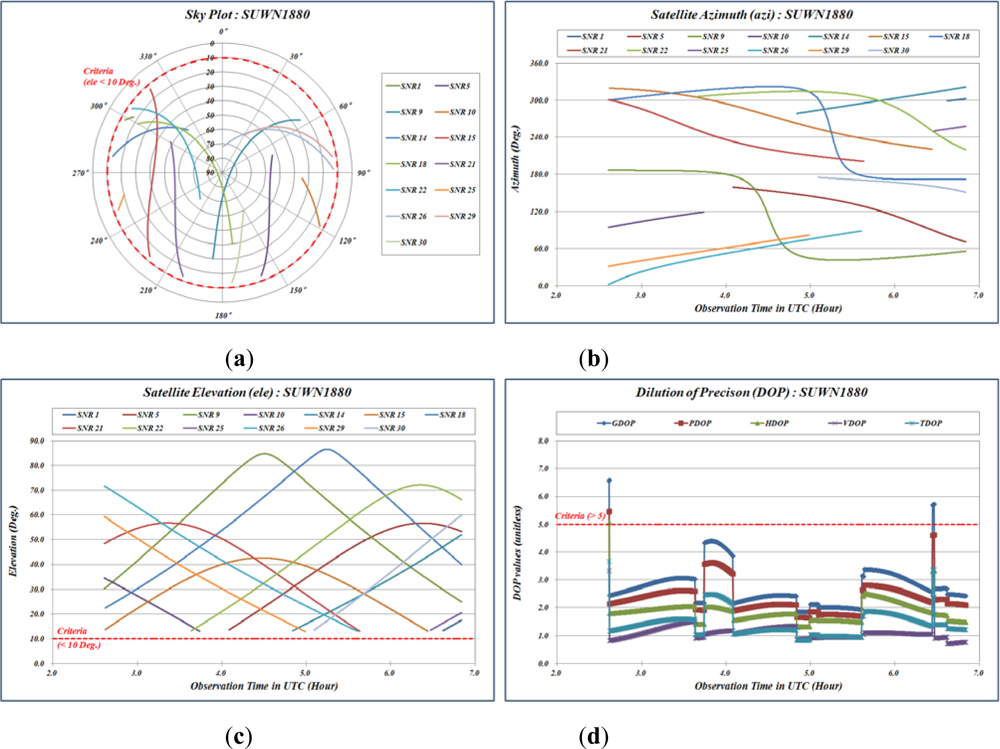
Figure 4.
Quality control indicators related to geometric arrangement. (a) Sky plot of observed satellite. (b) Satellite azimuths. (c) Satellite elevations. (d) DOPs.
Figure 4.
Quality control indicators related to geometric arrangement. (a) Sky plot of observed satellite. (b) Satellite azimuths. (c) Satellite elevations. (d) DOPs.

Figure 5.
Quality control indicators related to multi-path effects. (a) Time-series plots of MP1 at each observation epoch. (b) Time-series plots of MP2 at each observation epoch.
Figure 5.
Quality control indicators related to multi-path effects. (a) Time-series plots of MP1 at each observation epoch. (b) Time-series plots of MP2 at each observation epoch.

Figure 6.
Quality control indicators related to ionospheric effects. (a) Time-series plots of ion at each observation epoch. (b) Time-series plots of iod at each observation epoch.
Figure 6.
Quality control indicators related to ionospheric effects. (a) Time-series plots of ion at each observation epoch. (b) Time-series plots of iod at each observation epoch.

Figure 7.
Quality control indicators related to cycle slip effects (cyc) as shown in the time-series plots at each observation epoch.
Figure 7.
Quality control indicators related to cycle slip effects (cyc) as shown in the time-series plots at each observation epoch.


Table 1.
Descriptions of abbreviations used in Klobuchar model [9].
| Terms | Description | Terms | Description |
|---|---|---|---|
| φR, λR | Geodetic latitude and longitude of receiver | αn, γn | Broadcast ionospheric coefficients |
| azi, ele | Azimuth and elevation angle of satellite | td | GPS time [s] |
| P | A | ||
| x | ψ | ||
| ϕ | λR | ||
| F | D | ||
| φIP | t |
| QC Parameters | Skyplots | Multi-Paths | Cycle Slips | Ionospheric Delays | |||
|---|---|---|---|---|---|---|---|
| ele (°) | DOP | MP1 (m) | MP2 (m) | cyc | ion | iod | |
| Criteria | > 10 | < 5 | < 1.0 | < 2.0 | < ±2.0 | < ±10 | < ±0.3 |
| Allowance (%) | 90.0 | 90.0 | 90.0 | 90.0 | 90.0 | 80.0 | 80.0 |
| Days | Percentage of Criteria (%) | Comparison between Published and Daily Coordinate (m) | ||||||||
|---|---|---|---|---|---|---|---|---|---|---|
| ele | DOP | MP1 | MP2 | cyc | ion | iod | Daily Coord (m). | Precision of Daily Result (1σ) | Difference | |
| 1 | 93.29 | 100 | 93.89 | 95.05 | 88.48 | 83.57 | 94.35 | X : −3062022.8898 | ±0.0069 | 0.0175 |
| Y : 4055448.0180 | ||||||||||
| Z : 3841818.2516 | ||||||||||
| 2 | 93.34 | 100 | 94.46 | 95.37 | 90.99 | 86.80 | 94.77 | X: −3062022.8884 | ±0.0048 | 0.0075 |
| Y: 4055448.0098 | ||||||||||
| Z: 3841818.2510 | ||||||||||
| 3 | 93.32 | 100 | 94.42 | 95.33 | 90.90 | 86.14 | 94.61 | X: −3062022.8875 | ±0.0058 | 0.0086 |
| Y: 4055448.0092 | ||||||||||
| Z: 3841818.2514 | ||||||||||
| 4 | 93.26 | 100 | 94.26 | 95.28 | 90.46 | 84.42 | 94.99 | X: −3062022.8880 | ±0.0059 | 0.0088 |
| Y: 40555448.0063 | ||||||||||
| Z: 3841818.2486 | ||||||||||
| 5 | 93.21 | 100 | 94.03 | 95.01 | 88.56 | 82.89 | 94.55 | X: −3062022.8862 | ±0.0064 | 0.0141 |
| Y: 4055448.0104 | ||||||||||
| Z: 3841818.2559 | ||||||||||
Share and Cite
MDPI and ACS Style
Lee, D.; Cho, J.; Suh, Y.; Hwang, J.; Yun, H. A New Window-Based Program for Quality Control of GPS Sensing Data. Remote Sens. 2012, 4, 3168-3183. https://doi.org/10.3390/rs4103168
AMA Style
Lee D, Cho J, Suh Y, Hwang J, Yun H. A New Window-Based Program for Quality Control of GPS Sensing Data. Remote Sensing. 2012; 4(10):3168-3183. https://doi.org/10.3390/rs4103168
Chicago/Turabian StyleLee, Dongha, Jaemyoung Cho, Yongcheol Suh, Jinsang Hwang, and Hongsik Yun. 2012. "A New Window-Based Program for Quality Control of GPS Sensing Data" Remote Sensing 4, no. 10: 3168-3183. https://doi.org/10.3390/rs4103168