Downscaling Land Surface Temperature in an Urban Area: A Case Study for Hamburg, Germany


1
KlimaCampus Hamburg, University of Hamburg, Bundesstraße 55, D-20146 Hamburg, Germany
2
Institute of Geophysics, University of Hamburg, Bundesstraße 55, D-20146 Hamburg, Germany
3
Centre of excellence Space-Si, Aškerčeva 12, SI-1000 Ljubljana, Slovenia
*
Author to whom correspondence should be addressed.
Remote Sens. 2012, 4(10), 3184-3200; https://doi.org/10.3390/rs4103184
Submission received: 2 August 2012
/
Revised: 10 October 2012
/
Accepted: 12 October 2012
/
Published: 19 October 2012
(This article belongs to the Special Issue Thermal Remote Sensing Applications: Present Status and Future Possibilities)
Abstract
:Monitoring of (surface) urban heat islands (UHI) is possible through satellite remote sensing of the land surface temperature (LST). Previous UHI studies are based on medium and high spatial resolution images, which are in the best-case scenario available about four times per day. This is not adequate for monitoring diurnal UHI development. High temporal resolution LST data (a few measurements per hour) over a whole city can be acquired by instruments onboard geostationary satellites. In northern Germany, geostationary LST data are available in pixels sized 3,300 by 6,700 m. For UHI monitoring, this resolution is too coarse, it should be comparable instead to the width of a building block: usually not more than 100 m. Thus, an LST downscaling is proposed that enhances the spatial resolution by a factor of about 2,000, which is much higher than in any previous study. The case study presented here (Hamburg, Germany) yields promising results. The latter, available every 15 min in 100 m spatial resolution, showed a high explained variance (R2: 0.71) and a relatively low root mean square error (RMSE: 2.2 K). For lower resolutions the downscaling scheme performs even better (R2: 0.80, RMSE: 1.8 K for 500 m; R2: 0.82, RMSE: 1.6 K for 1,000 m).
1. Introduction
Increasing urbanization has caused changes in the heat balance in densely built urban areas [1–3]. In such cases, both mean air temperature and land surface temperature (LST) in the urban centers are usually higher than their respective temperatures in the rural surroundings. This phenomenon is known as urban heat island (UHI) [4–6]. Recent studies show that the development of UHI can be monitored using thermal remote sensing [7–12]. Remote sensing has a great advantage over in situ measurements. Instead of measurements at irregularly spaced point locations, remote sensing provides UHI with a quasi continuous monitoring of surfaces [13]. However, remote sensing of urban climates is restricted by several factors [14,15]. In particular, only the surface temperature UHI (also SUHI, here further referred to as UHI) can be directly monitored by remote sensing, which can largely differ from the canopy layer UHI. Another general problem of the satellite remote sensing is the lack of data having both high spatial and temporal resolution; a recent review of available sensors is given by Tomlison et al. [16].
In terms of UHI monitoring, a spatial resolution of 1 km allows coarse scale temperature mapping and limits the analysis of relationships between the UHI and in situ measurements of air temperature [17]. The highest spatial resolutions of spaceborn LST sensors are about 100 m, which would be much more appropriate, because it is a good approximation for an average width of a building block. Satellite instruments that retrieve data in such resolutions are the Advanced Spaceborne Thermal Emission and Reflection Radiometer (ASTER; spatial resolution of its thermal bands is 90 m) and Landsat (LS; spatial resolution of 120 m for LS 4 and 5, 60 m for LS 7 and 100 m for the coming LS 8 [18]). They fly on low earth orbiters with a relatively narrow swath and their revisit time is 16 days (eight days for ASTER including off-nadir acquisitions). Such a revisit time is too long to make these instruments suitable for the assessment of the diurnal evolution of UHI.
Instruments in the geostationary orbit like the Spinning Enhanced Visible Infra-Red Imager (SEVIRI) aboard Meteosat Second Generation (MSG) satellites on the other hand have appropriate temporal resolution but too poor spatial resolution (standard retrieval time of SEVIRI is 15 min; one SEVIRI pixel for the case study area of Hamburg is approximately 3,300 by 6,700 m large). Many studies are thus based on instruments in polar orbits that have wide swath (over 2,000 km) and a revisit time of approximately one day (one daytime and one night-time image). Such instruments have nominal spatial resolution of about 1,000 m, thus they are considered as a reasonable compromise between the two previously described options.
This paper examines the possibility of using an alternative approach based on the fusion of data with different temporal and spatial resolutions. Such an approach should provide results in high temporal (15 min) and high spatial (100 m) resolution. This should be possible as LST spatial distribution is well correlated with numerous parameters. Many of them can be observed by remote sensing in high spatial resolution. If the correlation between these parameters in high spatial resolution (HR) and low spatial resolution (LR) LST is known, LST in HR can be estimated. The factor of this downscaling was not larger than 100 in previous studies. This study aims to examine whether LST downscaling can be used with a higher downscaling factor in order to fulfill the needs of urban climatology (Section 2.1). Furthermore, it is investigated which predictors are most suitable to implement such a downscaling scheme and how the errors depend on the target resolution (Section 3). At the end possible improvements are discussed (Section 4).
2. Data and Methodology
2.1. LST Downscaling
Downscaling, image fusion, spatial sharpening and disaggregation are known methods to “improve” the spatial resolution of the input data using predictors of higher spatial resolution. In the first attempts of image fusion, the goal was the production of sharper multispectral images based on information obtained from the panchromatic band (e.g., [19–21] describe how to merge data from various instruments). In recent years, some studies proposed resolution improvement (from image sharpening to downscaling) for certain physical or ecological parameters. For instance, Kaheil and Creed [22] have improved the spatial resolution of wet areas and boreal landscapes; Zurita-Milla et al. [23] enhanced MERIS data for the vegetation seasonal dynamics monitoring to 25 m spatial resolution, and statistical and dynamical downscaling are used in meteorology to improve meteorological model outputs [24,25].
Therefore, LST downscaling is possible using physical or statistical based methods. Among physical based LST downscaling methods, the dual band method, often used in thermal anomaly monitoring [26], is the most common. With this method the percentage of thermally anomalous pixel coverage and the anomaly’s temperature can be estimated. However, the method yields no solution regarding the position of the anomaly. Another physical based LST downscaling method assumes that the data to be downscaled are isothermal, thus one can estimate subpixel emissivity and afterwards subpixel LST iteratively [27].
More common are statistical based methods. Most of them rely on the linear correlation between predictors (see following paragraph) and LST, e.g., [28–30]. Dominguez et al. [31] applied exponential functions to the predictors before applying the linear regression. Zakšek and Oštir [32] first performed principal component analysis over their predictors and then applied linear regression to the principal components. Zhou et al. [11] used support vector machine regression to determine the relationship between LST and predictors.
Statistically based downscaling can only be successful if appropriate HR predictors are available. Many biophysical parameters are well correlated to the LST spatial distribution. As most of them can be observed in finer resolution than LST, they are suitable as downscaling predictors. The most renowned is the negative correlation between LST and normalized difference vegetation index (NDVI) [29,30,33–37]. Merlin et al. [38] proposed to enhance the correlation between NDVI and LST using the temperature difference between photosynthetically and non-photosynthetically active vegetation. It is also possible to employ land cover data. Weng et al. [39] derived the vegetation fraction from ETM+ images; LST was better correlated with vegetation fraction than with NDVI. Yuan and Bauer [40] made a similar analysis but correlated the fraction of impervious surface area (soil sealing) that is strongly positive correlated to the LST in urban areas. Stathopoulou and Cartalis [41] showed that emissivity and season-coincident LST are also well correlated with the measured LST. It was also shown that there is a distinct correlation between water surfaces in urban areas and UHI [10,32]. Zhou et al. [11] reported a good correlation between some standard meteorological observations (atmospheric aerosol optical depth, relative humidity, sunshine duration, and precipitation) and LST. Bechtel [42] proposed annual cycle parameters (ACP) from multitemporal LST data as downscaling predictors. The utilization of LST data for LST downscaling might seem circular at the first glance. However, these predictors are independent and can be processed from globally available free Landsat data. Another option is the use of principal components of the multitemporal LST data. To conclude, all the listed parameters and all further parameters that are related to urban climatic processes like multispectral data (albedo) or morphological parameters (building geometry and irradiation) can be considered as LST downscaling predictors.
2.2. Case Study Area
The Southern part of Hamburg, Germany (53.38–53.63°E, 9.75–10.38°N) was chosen for the case study. It comprises the river Elbe (from South-East to North-West), rural areas with a high percentage of agricultural land use, forested areas in the Southwest and East and most of the city of Hamburg including the port areas (in the center), the central business district north of the river Elbe in the center as well as urban areas of different building densities (ranging from single family houses to very compact morphologies). Hamburg has a population of about 1.8 million inhabitants and is situated in the northern German lowland between the North Sea and the Baltic Sea. The domain of the study was limited by the availability of the morphological data (see below).
2.3. Data
2.3.1. Predictors
The entire set of 296 predictors was processed from different sensors and data sources. All predictors were first prepared on a 100 m UTM grid. For further analysis the predictors were resampled to lower resolutions between 200 m and 1,000 m in 100 m steps using an area weighted average. The spatial resolution of 100 m is appropriate because it is approximately equal to the width of a building block in a city. Coarser resolutions are more suitable for monitoring broader areas like city districts.
Topographic predictors derived from NEXTMap® Interferometric Synthetic Aperture Radar (IFSAR) data include simple statistics of the height distribution [43] as well as a morphological opening and closing profile, which includes spatial information about spacing and texture of buildings and other objects [44,45].
Multispectral predictors were derived from multitemporal data from the Thematic Mapper (TM) on board Landsat 4 and 5 and the Enhanced Thematic Mapper Plus (ETM+) on board Landsat 7. Since the predictors are only used in empirical models, calibration, atmospheric correction and conversion to reflectance were not considered necessary [46] and the raw digital numbers were applied. Bands 3 (RED) and 4 (NIR) were used to calculate the Normalized Differenced Vegetation Index (NDVI). The thermal infrared (TIR) acquisitions from multitemporal TM and ETM+ data (TIR band: 10.4–12.5 μm) were also included as predictors and several aggregated parameters were calculated. These include the two annual cycle parameters (ACP) mean annual surface temperature (MAST) and yearly amplitude of surface temperature (YAST) [47] as well as the best five principle components of all TIR scenes.
Further, some land cover data were included, more specifically the proportion of water per pixel (watershare) from a classification, the soil sealing from the EEA’s Fast Track Service Precursor Sealing Product “European Mosaic” (soilseal) and the percentage of larger roads as estimated from OpenStreetMap vector data.
2.3.2 LST Data
For calibration of the downscaling scheme the LSA SAF operational LST product was used. Their LST is produced every 15 min for cloud-free pixels [48]. SEVIRI TIR channels at 10.8 and 12.0 μm are applied to the generalized split-window algorithm [49]. The identification of pixels including the clouds is based on the Nowcasting and Very Short Range Forecasting SAF software [50]. The general accuracy of the LST product is below 2 K [48,51]. The quality of the derived LST mainly depends on the cloud detection accuracy, but also on the sensor performance, the accuracy of atmospheric corrections as well as the spectral variation in emissivities of different land-surface elements [51,52]. A significant parameter for LST accuracy is land surface heterogeneity, which can produce a significant variation in LST measurements.
The independent HR LST used for validation came from ASTER on board the Terra satellite. It retrieves data approximately 15 min after LS 7 in the same orbit. ASTER measures five thermal bands (between 8 and 11 μm) at 90 m horizontal resolution. Its LST product is calculated with the “temperature and emissivity separation algorithm” [53]. Although a campaign was launched for the entire summer of 2011, the request resulted in only one cloud free acquisition that covers the entire area of interest dating from 2 August 2011. The original swath data were first projected to UTM, then rasterized in 15 m resolution with nearest neighbor interpolation, and finally resampled to 100 m resolution (the same grid as the predictors) using area weighted average with SAGA GIS ( http://saga-gis.org/). This method ensures a minimum data loss and was found to be superior to a Multilevel B-Spline interpolation.
2.4. Used Methods
2.4.1. Spatial Aggregation of Predictors to the SEVIRI Grid
Downscaling starts with the aggregation of HR predictors to the same grid as LR LST. The input LST is given for a SEVIRI pixel that has an “irregular” shape according to the HR predictors in UTM projection. Instead of a simple geometrical resampling, the predictors were aggregated using the point spread function (PSF) of the sensor [54]. PSF was approximated by a Gaussian function in the proposed approach. Thus, the distances to a particular pixel center of SEVIRI LST were used to compute weights that express the influence of the PSF. The weights are normalized to a sum of one within each SEVIRI pixel. Therefore, those HR pixels that are closer to the centers of the SEVIRI pixels, have a greater influence on the aggregation results than pixels positioned in the corners of the SEVIRI pixels. To aggregate the predictors’ values to one SEVIRI pixel, it is necessary to sum all the products of the corresponding HR predictors and their normalized weights.
2.4.2. Selection of Suitable Predictors
To find optimal predictors for the downscaling scheme, the performances of different predictor sets were compared. First, predictors were grouped according to their origin in order to evaluate which data sources contain relevant information. Then, single predictors with high potential were tested and sets were combined by expert knowledge. Further sets were compiled by different feature selection algorithms (described in the following three paragraphs) in order to eliminate covariant, irrelevant, redundant and noisy variables and find the most meaningful predictors.
The Minimum Redundancy Maximal Relevance approach (MRMR) was first used in bioinformatics for genome classification [55]. The algorithm is based on the fact that the most relevant individual features are likely to be highly redundant and hence additional predictors might not significantly improve the result. For optimum choice, the relevance for the target variable and the redundancy with the prior selected predictors are combined in a single (Mutual Information Quotient) criterion. As the algorithm was developed for classification of ordinal data, the predictors and LST data were discretized into ten classes for the selection.
Forward selection is a linear step-by-step algorithm that has been successfully used by many researchers in order to build robust prediction models [56,57]. In this approach, which is based on a linear regression model; the first step to sort the explanatory variables according to their correlation with the dependent variable. Then, the predictor that is best correlated with the dependent variable is selected as the first input. The remaining variables are added one by one as the second input according to their correlation with the output. The variable that increases most significantly the explained model variance (R2) is selected as the second input. This step is repeated for all predictors. Finally, among the obtained subsets, the subset with optimum R2 is selected as the model input subset. This means adding further variables to this subset does not significantly increase the R2 [57].
An alternative to MRMR and forward selection would be the principal component analysis (PCA) as applied in LST downscaling by Zakšek and Oštir [32]. PCA decreases the possible set of predictors to some highest ranking principal components (PC) describing the most variability in the whole set of the predictors.
2.4.3. Downscaling
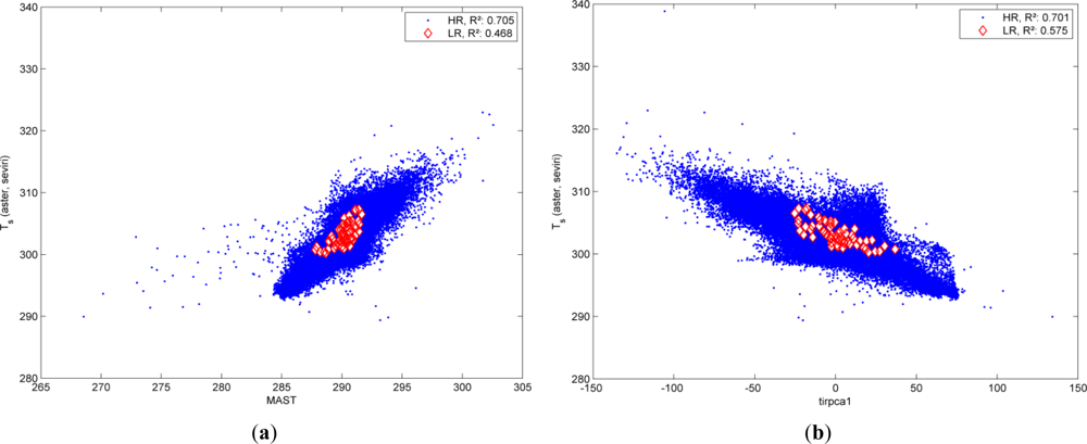
Figure 1 explains the basic principle of statistical downscaling. It is assumed that the predictors are correlated to LST in a similar manner in LR as well as HR spatial domain. Therefore, a linear regression model, calibrated from the (upscaled) LR predictor sets, and measured LR LST should be suitable to explain HR LST distribution from HR predictors. The example in Figure 1 shows that:
- a predictor, in the example MAST Figure 1(a) and the first TIR PC Figure 1(b) are used, is correlated to LST in both LR (red) and HR (blue) domain.
- the variance in the LR domain is much lower for both predictors and dependent variable (which is plausible since the upscaling is essentially a low pass filtering operation), and
- the linear relation is similar for both domains.
Hence, linear functions are calibrated by Multiple Regression in the LR domain and then applied to the HR predictors. However, it can also be seen that the linear equation only explains a part of the variance and that certain areas have a divergent thermal behavior.
3. Results
3.1. Linear Regression with Different Predictor Sets
The results of the Linear Regression models with different predictor sets are presented in Table 1. Generally, models with large predictor sets tended to overfit. This resulted in a high level of explained variance (R2) for the training set in the LR domain but produced some high errors (mean absolute error (MAE), root mean square error (RMSE)) as well as small R2 for the independent validation data in the HR domain. Conversely, using regression with merely a single TIR predictor (selected from the highest correlation in LR) reached an RMSE of 2.63 K and an R2 of 0.53 for the HR validation data. The ACP predictors performed much better with RMSE = 2.17 K and R2 = 0.71 for MAST only and RMSE = 2.21 and R2 = 0.68 for MAST and YAST. Comparably, the principal components of all TIR scenes reached very good results in the downscaling scheme, with only the first component slightly outperforming larger sets (RMSE = 2.17, R2 = 0.70 for the first PC, RMSE = 2.37, R2 = 0.63 for the first three ranking PC, and RMSE = 2.42, R2 = 0.61 for the first five ranking PC). The sets chosen by expert knowledge also performed quite well (RMSE = 2.35, R2 = 0.63 for “expert1”, containing of YAST, tirpca1, watershare, soilseal, NDVI from LS scene #LT41960231992178XXX02, the blue band from #LT51950232006185KIS00 and the TIR band from #LE71950232001227EDC00). The sets “expert2” and “expert3” consist of MAST for the one and tirpca1 for the other, supplemented by watershare, since the water pixels are believed to have a different thermal signature. Although both are among the best predictor sets (RMSE = 2.47 K, R2 = 0.57 and RMSE = 2.31 K, R2 = 0.65), the addition of watershare leads to a better fit in LR domain but a slightly higher error in the HR domain. The sets chosen by feature selection performed differently. While the smallest MRMR (TIR band from #LT51960232010155MOR01 and NIR from #LE71960232002093EDC00) set was still among the best (RMSE = 2.51 K, R2 = 0.54), the forward selection failed in selecting suitable downscaling predictor sets (RMSE = 4.18 K, R2 = 0.19 with 3 TIR bands, one green band and a morphological closing from the profile).
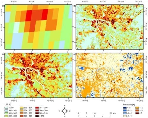
Hence, it can be stated that predictor sets should not be larger than a few predictors and that aggregated patterns of multitemporal thermal data are very powerful for downscaling LST. Figure 2 shows the results of the downscaling scheme with the ACP predictor set and the spatial distribution of the error compared with the ASTER validation data. The predicted LST pattern with high LST for the port, other industrial areas as well as the inner city and the coolest temperatures for the forests (Southwest and East) (Figure 2(c)) is much finer than the SEVIRI LST data (Figure 2(a)) and visually similar to the ASTER testing dataset (Figure 2(b)). The residuals (Figure 2(d)) are rather low for the urban areas and somewhat higher for forest and water areas and have a large variance for agricultural fields. Orange colors prevail, indicating an overestimation of the HR LST, which is consistent with the bias of approximately 1.3 K for all models in Table 1. The systematic errors can partly be related to differing water lines, phenology (especially different crop status in the agricultural areas) and land use change.
The equation presented below for the ACP downscaling is evidently only valid for the specific acquisition and the coefficients are in fact a function of time:
3.2. Downscaling to Different Resolutions
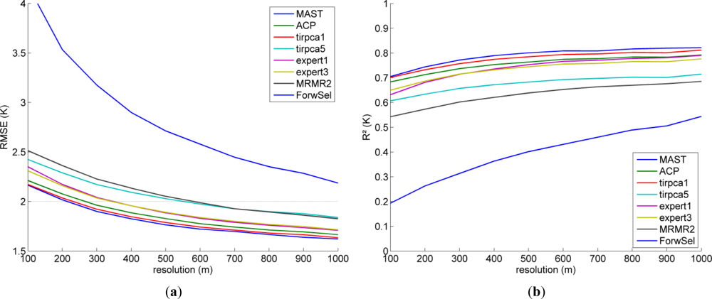
Since the downscaling factor between SEVIRI and ASTER is quite large (approximately a factor of 33 in East-West direction and 67 in North-South), both predictors and testing data were resampled to lower resolutions between 200 m and 1,000 m using an area weighted average in order to evaluate the performance of the scheme for different resolutions. Figure 3(a) shows the validation RMSE in different resolutions. As expected, the error decreases with decreasing resolution and an RMSE of 2 K (black dotted line) was reached at a target resolution between 200 m and 300 m for the better predictor sets. Accordingly, the explained variance of the validation dataset displayed in Figure 3(b) increases. The order among the predictor sets was essentially preserved and MAST, tirpca1 and ACP were the best predictor sets for all resolutions. However, the predictor set “expert1” (with seven predictors) performed better in relation to the others at lower resolutions.
4. Discussion
Regarding the large downscaling factor between SEVIRI and ASTER data, the results of the Hamburg case study are very promising. Three proposed predictor sets reached an RMSE of about 2.2 K and an explained variance of about 0.7. An RMSE of less than 2 K was reached by three predictor sets at a target resolution of 300 m, at 1,000 m resolution RMSEs of about 1.65 K and R2 of about 0.8 were reached. These results are very good compared with the accuracy of the SEVIRI LST retrieval of 2 K [48,51]. In the past, only a few studies were dedicated to downscaling of LST in the urban areas. Liu and Pu [27] reached a better R2 (0.77) for their Yokohama (Japan) case study. However, they downscaled from MODIS to ASTER resolution, which is a much smaller downscaling factor (about 100); comparable results were achieved in this study for a resolution of 300 to 400 m, which is still a higher downscaling factor. The downscaling from ASTER to 10 m resolution in San Juan (Puerto Rico) suggested by Dominguez et al. [31] also resulted in higher explained variance (R2 = 0.81) and higher error (RMSE = 2.8 K) than in this study. Stathopoulou and Cartalis [41] downscaled AVHRR to LS TM resolution in Athens (Greece) with much higher errors than in this study (RMSE = 4.9 K). We are aware of two studies that tried to downscale LST in urban areas using geostationary data. Zakšek and Oštir [32] downscaled the SEVIRI data to 1,000 m resolution for the urban areas of central Europe. Their correlation is very high (R = 0.97, which corresponds to an R2 of about 0.94) but their error is also higher than ours (RMSE = 2.5 K). Keramitsoglou [58] also downscaled SEVIRI data to 1,000 m resolution but for the area of Athens (Greece); 67% of the processed datasets exhibit correlation coefficient between 0.6 and 0.8.
Although the presented results are encouraging compared with the listed studies, improvements are still possible. The random error of the downscaling scheme is even much lower, if the large systematic bias of about 1.3 K for all models and resolutions is considered. Thus, the overall error could be substantially decreased if an independent estimate of the bias was available. The reason for the bias is the geometry of data retrieval. The geostationary SEVIRI views Europe from the South, thus it sees a remarkable share of southern vertical sides of objects. These are warmer, while northern facades of buildings are not seen by SEVIRI at all. On board a low Earth orbiter, ASTER can be used off-nadir at low angles and thus also often observes surfaces towards West or towards East, resulting in an azimuth dependent LST. However, the viewing geometry of ASTER is still “largely perpendicular” compared with SEVIRI (for instance a pointing angle of 5.71°for the used ASTER scene instead of almost 60° for SEVIRI). Hence, mostly horizontal objects (especially roofs and streets) are seen by ASTER. This bias can also be seen in the scatterplots in Figure 1 (higher intercept of the LR data) and is in acceptable agreement with previous studies. Trigo et al. for instance reported that the SEVIRI LST was about 2 K higher than MODIS LST for the Iberian Peninsula, Central Africa, and the Kalahari [51]. MODIS (terra) has a comparable viewing geometry to ASTER, since it flies on the same platform. The bias seemed to be largely independent from the tested resolutions (the mean bias of eight selected predictor sets was between 1.310 and 1.314 for all tested resolutions). Besides the geometrical influences, systematic errors due to a small time difference between SEVIRI and ASTER retrieval and different emissivity retrieval algorithms used in both products cannot be excluded.
In general, the aggregated TIR parameters (ACP, tirpca) turned out to be the most suitable predictors for LST downscaling and the sets selected by expert knowledge outperformed the automatic feature selection methods. Furthermore, the smallest predictor sets also resulted in the smallest errors. The predicted HR LST then just is a linear combination of few patterns. Since these parameters are essentially all derived from measurements at a similar time (and hence similar heating patterns), the downscaling is likely to perform less well for different times of the day. Unfortunately, ASTER validation data is mostly restricted to one acquisition time. Only a few night-time acquisitions are available (during the case study observation period, the night-time retrieval completely failed).
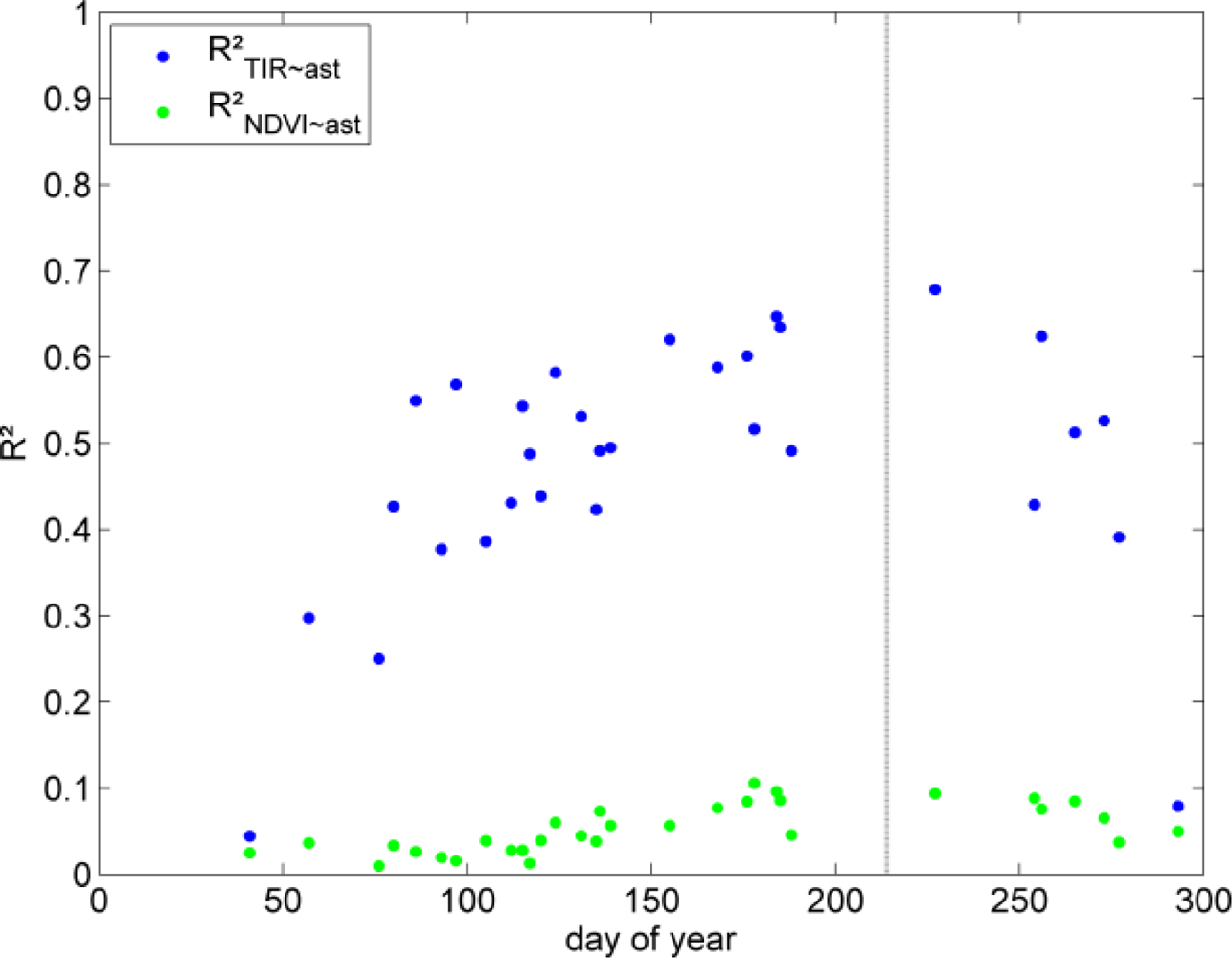
Heating patterns acquired during different seasons can be assumed to show comparable effects. Hence, the correlations between the ASTER LST and Landsat TIR data from different times of the year (also from different years) were investigated. In Figure 4 the correspondence between LST from ASTER and Landsat TIR (blue) as well as NDVI (green) from different days of the year are shown. The vertical line indicates the ASTER acquisition day and it can be seen that acquisitions from the same season have a higher R2 while the thermal patterns from winter acquisitions are substantially different. Hence, predictor sets of more than one pattern are expected to be more stable in order to produce heating patterns for different times of the day.
NDVI predictors were expected to be suitable for the downscaling scheme. The correlation between single NDVI predictors and ASTER LST (see also Figure 4) in the case study was, however, significantly lower than the values from literature (for instance 0.7 in [36]). This is a result of several factors. First, a large time lag between LST and NDVI is responsible for different phenological conditions that have a major influence on LST (Figure 4 shows a strong seasonal dependency between the variance of ASTER LST explained by NDVI). An additional analysis revealed that the explained variance of the NDVI predictors with the respective TIR patterns of the same day is much higher (R2 = 0.36). Secondly, NDVI should not be linearly upscaled but recomputed from the upscaled red and NIR bands. Thirdly and most importantly, the low correlations of the different NDVI result from the high fraction of water coverage in Hamburg. LST of the water bodies is largely dominated by their heat storage capacity as well as advection from upstream areas. For the given situation the water temperatures are lower than those of the vegetated areas. Conversely, water has a low NDVI like impervious surfaces (water bodies and adjacent sealed areas show LST deviations of more than 20 K). Hence, NDVI shows a much higher explained variance (e.g., R2 = 0.31 instead of R2 = 0.09 for scene #LT41960231989185XXX0) if the water pixels are excluded. Thus, we expect the fraction of active vegetation (besides those of impervious surfaces and water) to be a better LST predictor than NDVI. This is in agreement with Weng et al. [39], who argue that LST is more correlated to vegetation fraction than NDVI.
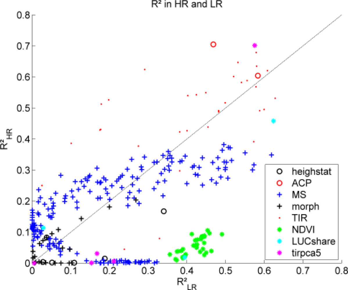
To answer the question which predictors are suitable for the downscaling scheme, the explained variances of single predictors in LR and HR were compared. The results are displayed in Figure 5. It can be seen that NDVI shows a much higher R2 in LR domain, which is again a consequence of the water bodies that cover only small proportions of single SEVIRI pixels. Hence, the basic assumption of the downscaling is not fulfilled for these predictors. Conversely, the ACP (red circles), the first TIR PC (magenta asterix at lower left), and soilseal (cyan, upper right) show very high R2 in both HR and LR, which are almost identical (indicated by black dotted line). Hence, they fulfill the basic assumption and are suitable predictors, which is in good agreement with their results in Table 1. The multispectral data partly suffers from the same problem as NDVI, while most of the morphological and heighstat features (besides the minimum height) and some of the additional TIR PCs explain only little variance. This leaves only a small number of the tested predictors that are really suitable. The same conclusion was also underpinned by an additional experiment with PCs calculated from the complete predictor set. The first PC, which explained about 52% of the overall variability, was only very weakly correlated to ASTER LST (R = 0.27) indicating that a large number of predictors are rather ineffective.
5. Conclusions
This study demonstrates that it is possible to downscale land surface temperature (LST) for a factor of about 2,000. By this spatial improvement the resulting accuracy (root mean square error = 2.2 K) remained comparable to the accuracy of LST retrieved by geostationary satellites. The most suitable downscaling predictors are aggregated from thermal infrared data. A surprising outcome of the case study is that the normalized difference vegetation index failed to explain the LST variability. Eventually, we aim to achieve a time dependent downscaling scheme, which presupposes validation data from in situ measurements or thermography in high temporal resolution. Such complete diurnal cycles of LST at 100 m could be used to study the surface urban heat island and the specific thermal behavior of different urban morphologies, to validate mesoscale urban models and to derive material specific properties like thermal inertia.
Acknowledgments
We are grateful to H. Peng and colleagues for the MRMR code, the Machine Learning Group at the University of Waikato for WEKA, and Jürgen Böhner and Olaf Conrad for SAGA-GIS. Further, we thank the NASA, the EEA, Open StreetMap, and Intermap Technologies for the predictor raw data and LSA SAF for the SEVIRI LST data. For his patience and helpful advice with the ASTER acquisition request we thank Tetsuro Nishimura. For proof reading and useful advice on the comprehensibility of the manuscript we thank Claire Nattrass, Leonie Pick, Eleonore Rauch and Michael Bock.
The Cluster of Excellence CliSAP (EXC177) is hosted by the KlimaCampus and funded by the German Federal and the Hamburg state Government. This research has been supported also by a grant from the German Science Foundation (DFG) number ZA659/1-1. The Centre of Excellence for Space Sciences and Technologies SPACE-SI is an operation partly financed by the European Union, European Regional Development Fund and Republic of Slovenia, Ministry of Higher Education, Science and Technology.
References
- Jin, M.S.; Kessomkiat, W.; Pereira, G. Satellite-observed urbanization characters in Shanghai, China: Aerosols, urban heat island effect, and land-atmosphere interactions. Remote Sens 2011, 3, 83–99. [Google Scholar]
- Xiong, Y.; Huang, S.; Chen, F.; Ye, H.; Wang, C.; Zhu, C. The impacts of rapid urbanization on the thermal environment: A remote sensing study of Guangzhou, South China. Remote Sens 2012, 4, 2033–2056. [Google Scholar]
- Frey, C.M.; Parlow, E. Flux measurements in Cairo. Part 2: On the determination of the spatial radiation and energy balance using aster satellite data. Remote Sens 2012, 4, 2635–2660. [Google Scholar]
- Kim, Y.-H.; Baik, J.-J. Spatial and temporal structure of the urban heat island in Seoul. J. Appl. Meteor 2005, 44, 591–605. [Google Scholar]
- Oke, T.R. City size and the urban heat island. Atmos. Environ 1973, 7, 769–779. [Google Scholar]
- Yow, D.M. Urban heat islands: Observations, impacts, and adaptation. Geogr. Compass 2007, 1, 1227–1251. [Google Scholar]
- Weng, Q. Thermal infrared remote sensing for urban climate and environmental studies: Methods, applications, and trends. ISPRS J. Photogramm 2009, 64, 335–344. [Google Scholar]
- Hamdi, R. Estimating urban heat island effects on the temperature series of uccle (Brussels, Belgium) using remote sensing data and a land surface scheme. Remote Sens 2010, 2, 2773–2784. [Google Scholar]
- Liu, L.; Zhang, Y. Urban heat island analysis using the landsat tm data and aster data: A case study in Hong Kong. Remote Sens 2011, 3, 1535–1552. [Google Scholar]
- Rinner, C.; Hussain, M. Toronto’s urban heat island—Exploring the relationship between land use and surface temperature. Remote Sens 2011, 3, 1251–1265. [Google Scholar]
- Zhou, J.; Chen, Y.; Wang, J.; Zhan, W. Maximum nighttime urban heat island (UHI) intensity simulation by integrating remotely sensed data and meteorological observations. IEEE J. Sel. Top. Appl. Earth Obs. Remote Sens 2011, 4, 138–146. [Google Scholar]
- Weng, Q.; Rajasekar, U.; Hu, X. Modeling urban heat islands and their relationship with impervious surface and vegetation abundance by using aster images. IEEE Trans. Geosci. Remote Sens 2011, 49, 4080–4089. [Google Scholar]
- Fabrizi, R.; Bonafoni, S.; Biondi, R. Satellite and ground-based sensors for the urban heat island analysis in the city of Rome. Remote Sens 2010, 2, 1400–1415. [Google Scholar]
- Roth, M.; Oke, T.R.; Emery, W.J. Satellite-derived urban heat islands from three coastal cities and the utilization of such data in urban climatology. Int. J. Remote Sens 1989, 10, 1699–1720. [Google Scholar]
- Voogt, J.A.; Oke, T.R. Thermal remote sensing of urban climates. Remote Sens. Environ 2003, 86, 370–384. [Google Scholar]
- Tomlinson, C.J.; Chapman, L.; Thornes, J.E.; Baker, C. Remote sensing land surface temperature for meteorology and climatology: A review. Meteorol. Appl 2011, 18, 296–306. [Google Scholar]
- Li, J.; Song, C.; Cao, L.; Zhu, F.; Meng, X.; Wu, J. Impacts of landscape structure on surface urban heat islands: A case study of Shanghai, China. Remote Sens. Environ 2011, 115, 3249–3263. [Google Scholar]
- Schott, J.; Gerace, A.; Brown, S.; Gartley, M.; Montanaro, M.; Reuter, D.C. Simulation of image performance characteristics of the landsat data continuity mission (LDCM) thermal infrared sensor (TIRS). Remote Sens 2012, 4, 2477–2491. [Google Scholar]
- Price, J.C. Combining multispectral data of differing spatial resolution. IEEE Trans. Geosci. Remote Sens 1999, 37, 1199–1203. [Google Scholar]
- Švab, A.; Oštir, K. High-resolution image fusion: Methods to preserve spectral and spatial resolution. Photogramm. Eng. Remote Sensing 2006, 72, 565–572. [Google Scholar]
- Zhukov, B.; Oertel, D.; Lanzl, F.; Reinhackel, G. Unmixing-based multisensor multiresolution image fusion. IEEE Trans. Geosci. Remote Sens 1999, 37, 1212–1226. [Google Scholar]
- Kaheil, Y.H.; Creed, I.F. Detecting and downscaling wet areas on boreal landscapes. IEEE Geosci. Remote Sens. Lett 2009, 6, 179–183. [Google Scholar]
- Zurita-Milla, R.; Kaiser, G.; Clevers, J.G.P.W.; Schneider, W.; Schaepman, M.E. Downscaling time series of MERIS full resolution data to monitor vegetation seasonal dynamics. Remote Sens. Environ 2009, 113, 1874–1885. [Google Scholar]
- Denis, B.; Laprise, R.; Caya, D.; Côté, J. Downscaling ability of one-way nested regional climate models: The big-brother experiment. Clim. Dynam 2002, 18, 627–646. [Google Scholar]
- Gangopadhyay, S.; Clark, M.; Rajagopalan, B. Statistical downscaling using K-nearest neighbors. Water Resour. Res 2005, 41, W02024. [Google Scholar]
- Dozier, J. A method for satellite identification of surface temperature fields of subpixel resolution. Remote Sens. Environ 1981, 11, 221–229. [Google Scholar]
- Liu, D.; Pu, R. Downscaling thermal infrared radiance for subpixel land surface temperature retrieval. Sensors 2008, 8, 2695–2706. [Google Scholar]
- Inamdar, A.K.; French, A. Disaggregation of GOES land surface temperatures using surface emissivity. Geophys. Res. Lett 2009, 36, L02408. [Google Scholar]
- Inamdar, A.K.; French, A.; Hook, S.; Vaughan, G.; Luckett, W. Land surface temperature retrieval at high spatial and temporal resolutions over the southwestern United States. J. Geophys. Res 2008, 113, D07107. [Google Scholar]
- Kustas, W.P.; Norman, J.M.; Anderson, M.C.; French, A.N. Estimating subpixel surface temperatures and energy fluxes from the vegetation index-radiometric temperature relationship. Remote Sens. Environ 2003, 85, 429–440. [Google Scholar]
- Dominguez, A.; Kleissl, J.; Luvall, J.C.; Rickman, D.L. High-resolution urban thermal sharpener (HUTS). Remote Sens. Environ 2011, 115, 1772–1780. [Google Scholar]
- Zakšek, K.; Oštir, K. Downscaling land surface temperature for urban heat island diurnal cycle analysis. Remote Sens. Environ 2012, 117, 114–124. [Google Scholar]
- Prihodko, L.; Goward, S.N. Estimation of air temperature from remotely sensed surface observations. Remote Sens. Environ 1997, 60, 335–346. [Google Scholar]
- Czajkowski, K.P.; Goward, S.N.; Stadler, S.J.; Walz, A. Thermal remote sensing of near surface environmental variables: Application over the Oklahoma mesonet. Prof. Geogr 2000, 52, 345–357. [Google Scholar]
- Agam, N.; Kustas, W. P.; Anderson, M.C.; Li, F.; Neale, C.M.U. A vegetation index based technique for spatial sharpening of thermal imagery. Remote Sens. Environ 2007, 107, 545–558. [Google Scholar]
- Stisen, S.; Sandholt, I.; Nørgaard, A.; Fensholt, R.; Eklundh, L. Estimation of diurnal air temperature using MSG SEVIRI data in West Africa. Remote Sens. Environ 2007, 110, 262–274. [Google Scholar]
- Zakšek, K.; Schroedter-Homscheidt, M. Parameterization of air temperature in high temporal and spatial resolution from a combination of the SEVIRI and MODIS instruments. ISPRS J. Photogramm 2009, 64, 414–421. [Google Scholar]
- Merlin, O.; Duchemin, B.; Hagolle, O.; Jacob, F.; Coudert, B.; Chehbouni, G.; Dedieu, G.; Garatuza, J.; Kerr, Y. Disaggregation of MODIS surface temperature over an agricultural area using a time series of Formosat-2 images. Remote Sens. Environ 2010, 114, 2500–2512. [Google Scholar] [Green Version]
- Weng, Q.; Lu, D.; Schubring, J. Estimation of land surface temperature-vegetation abundance relationship for urban heat island studies. Remote Sens. Environ 2004, 89, 467–483. [Google Scholar]
- Yuan, F.; Bauer, M.E. Comparison of impervious surface area and normalized difference vegetation index as indicators of surface urban heat island effects in Landsat imagery. Remote Sens. Environ 2007, 106, 375–386. [Google Scholar]
- Stathopoulou, M.; Cartalis, C. Downscaling AVHRR land surface temperatures for improved surface urban heat island intensity estimation. Remote Sens. Environ 2009, 113, 2592–2605. [Google Scholar]
- Bechtel, B. Robustness of annual cycle parameters to characterize the urban thermal landscapes. IEEE Geosci. Remote Sens. Lett 2012, 9, 876–880. [Google Scholar]
- Bechtel, B.; Langkamp, T.; Ament, F.; Bohner, J.; Daneke, C.; Gunzkofer, R.E.N.; Leitl, B.; Ossenbrugge, J.; Ringeler, A. Towards an urban roughness parameterisation using interferometric SAR data taking the metropolitan region of Hamburg as an example. Meteorol. Z 2011, 20, 29–37. [Google Scholar]
- Benediktsson, J.A.; Palmason, J.A.; Sveinsson, J.R. Classification of hyperspectral data from urban areas based on extended morphological profiles. IEEE Trans. Geosci. Remote Sens 2005, 43, 480–491. [Google Scholar]
- Bechtel, B.; Daneke, C. Classification of local climate zones based on multiple earth observation data. IEEE J. Sel. Top. Appl. Earth Obs. Remote Sens 2012, 5, 1191–1202. [Google Scholar]
- Song, C.; Woodcock, C.E.; Seto, K.C.; Lenney, M.P.; Macomber, S.A. Classification and change detection using Landsat TM data: When and how to correct atmospheric effects? Remote Sens. Environ 2001, 75, 230–244. [Google Scholar]
- Bechtel, B. Robustness of annual cycle parameters to characterize the urban thermal landscapes. IEEE Geosci. Remote Sens. Lett 2012, 9, 876–880. [Google Scholar]
- SAF LSA. Land Surface Temperature (15 mins). Available online: https://landsaf.meteo.pt/algorithms.jsp?seltab=0&starttab=0 (accessed on 18 June 2012).
- Wan, Z.; Dozier, J. A generalized split-window algorithm for retrieving land-surface temperature from space. IEEE Trans. Geosci. Remote Sens 1996, 34, 892–905. [Google Scholar]
- SAF NWC. MSG Cloud Products. Available online: http://www.nwcsaf.org/HD/MainNS.jsp (accessed on 18 June 2012).
- Trigo, I.F.; Monteiro, I.T.; Olesen, F.; Kabsch, E. An assessment of remotely sensed land surface temperature. J. Geophys. Res 2008, 113, D17108. [Google Scholar]
- Sun, D.; Pinker, R.T. Retrieval of surface temperature from the MSG-SEVIRI-observations: Part I. Methodology. Inter. J. Remote Sens 2007, 28, 5255–5272. [Google Scholar]
- Gillespie, A.; Rokugawa, S.; Matsunaga, T.; Cothern, J.S.; Hook, S.; Kahle, A.B. A temperature and emissivity separation algorithm for Advanced Spaceborne Thermal Emission and Reflection radiometer (ASTER) images. IEEE Trans. Geosci. Remote Sens 1998, 36, 1113–1126. [Google Scholar]
- Deneke, H.M.; Roebeling, R.A. Downscaling of METEOSAT SEVIRI 0.6 and 0.8 μm channel radiances utilizing the high-resolution visible channel. Atmos. Chem. Phys 2010, 10, 9761–9772. [Google Scholar]
- Peng, H.; Long, F.; Ding, C. Feature selection based on mutual information: Criteria of max-dependency, max-relevance, and min-redundancy. IEEE Trans. Patt. Anal. Mach. Int 2005, 27, 1226–1238. [Google Scholar]
- Chen, S.; Hong, X.; Harris, C.J.; Sharkey, P.M. Sparse Modelling Using Orthogonal Forward Regression with PRESS Statistic and Regularization. Available online: http://eprints.soton.ac.uk/259231/ (accessed on 28 June 2012).
- Noori, R.; Hoshyaripour, G.; Ashrafi, K.; Araabi, B.N. Uncertainty analysis of developed ANN and ANFIS models in prediction of carbon monoxide daily concentration. Atmos. Environ 2010, 44, 476–482. [Google Scholar]
- Keramitsoglou, I. Advanced Earth Observation Methodologies for the Study of the Thermal Environment of Cities. Proceedings of 2012 Second International Workshop on Earth Observation and Remote Sensing Applications (EORSA), Shanghai, China, 8–11 June 2012; pp. 11–15.
Figure 1.
Relation between dependent variable land surface temperature (LST) in high spatial resolution (HR) (blue) and low spatial resolution (LR) (red) domain and different predictors. (a) mean annual surface temperature (MAST) (b) first principal component of thermal infrared (TIR) data.
Figure 1.
Relation between dependent variable land surface temperature (LST) in high spatial resolution (HR) (blue) and low spatial resolution (LR) (red) domain and different predictors. (a) mean annual surface temperature (MAST) (b) first principal component of thermal infrared (TIR) data.

Figure 2.
(a) LR Spinning Enhanced Visible Infra-Red Imager (SEVIRI) land surface temperature (LST), (b) HR Advanced Spaceborne Thermal Emission and Reflection Radiometer (ASTER) LST, (c) Downscaling result for LST with ACP predictor set, (d) Spatial distribution of the error of the model compared with ASTER validation data.

Figure 3.
Resolution dependent performance of the downscaling scheme for different predictor sets. (a) root mean square error (RMSE) (K). (b) R2.
Figure 3.
Resolution dependent performance of the downscaling scheme for different predictor sets. (a) root mean square error (RMSE) (K). (b) R2.

Figure 4.
Variance in ASTER LST data (day indicated by dotted line) that can be explained by Landsat data (TIR and NDVI) from different seasons.
Figure 4.
Variance in ASTER LST data (day indicated by dotted line) that can be explained by Landsat data (TIR and NDVI) from different seasons.

Figure 5.
Explained variance R2 of single predictors with LST in LR and HR.


Table 1.
Downscaling accuracy with linear regression for different predictor sets. Number of predictors in the set (Num), explained variance (R2) of the model in LR domain, mean absolute error (MAE), root mean square error (RMSE), R2 and BIAS for the independent validation data in HR domain. Best predictor sets are highlighted blue.
| Predictor Set | Calibr. | Validation (HR) | ||||
|---|---|---|---|---|---|---|
| Name | Num | R2 (LR) | MAE (K) | RMSE (K) | R2 | BIAS (K) |
| predefined sets | ||||||
| heighstat | 6 | 0.722 | 4.31 | 6.09 | 0.04 | 1.40 |
| LUCshare | 3 | 0.634 | 2.23 | 2.96 | 0.33 | 1.33 |
| NDVI | 32 | 0.825 | 6.40 | 9.15 | 0.00 | 1.46 |
| TIR | 32 | 0.867 | 3.36 | 4.46 | 0.11 | 1.42 |
| single predictors | ||||||
| bestNDVI[lres] | 1 | 0.356 | 2.51 | 3.73 | 0.03 | 1.36 |
| bestTIR[lres] | 1 | 0.628 | 2.08 | 2.63 | 0.53 | 1.32 |
| aggregated LST predictors | ||||||
| MAST | 1 | 0.468 | 1.76 | 2.17 | 0.71 | 1.29 |
| ACP | 2 | 0.593 | 1.82 | 2.21 | 0.68 | 1.31 |
| tirpca1 | 1 | 0.575 | 1.79 | 2.17 | 0.70 | 1.31 |
| tirpca3 | 3 | 0.622 | 1.89 | 2.37 | 0.63 | 1.37 |
| tirpca5 | 5 | 0.633 | 1.89 | 2.42 | 0.61 | 1.38 |
| selected by expert knowledge | ||||||
| expert1 | 7 | 0.698 | 1.86 | 2.35 | 0.63 | 1.35 |
| expert2 | 2 | 0.514 | 1.85 | 2.47 | 0.57 | 1.34 |
| expert3 | 2 | 0.591 | 1.82 | 2.31 | 0.65 | 1.33 |
| feature selection algorithms | ||||||
| MRMR2 | 2 | 0.641 | 1.98 | 2.51 | 0.54 | 1.31 |
| MRMR6 | 6 | 0.702 | 2.03 | 2.64 | 0.52 | 1.35 |
| MRMR10 | 10 | 0.717 | 2.12 | 2.91 | 0.43 | 1.35 |
| ForwSel | 5 | 0.799 | 3.07 | 4.18 | 0.19 | 1.42 |
Share and Cite
MDPI and ACS Style
Bechtel, B.; Zakšek, K.; Hoshyaripour, G. Downscaling Land Surface Temperature in an Urban Area: A Case Study for Hamburg, Germany. Remote Sens. 2012, 4, 3184-3200. https://doi.org/10.3390/rs4103184
AMA Style
Bechtel B, Zakšek K, Hoshyaripour G. Downscaling Land Surface Temperature in an Urban Area: A Case Study for Hamburg, Germany. Remote Sensing. 2012; 4(10):3184-3200. https://doi.org/10.3390/rs4103184
Chicago/Turabian StyleBechtel, Benjamin, Klemen Zakšek, and Gholamali Hoshyaripour. 2012. "Downscaling Land Surface Temperature in an Urban Area: A Case Study for Hamburg, Germany" Remote Sensing 4, no. 10: 3184-3200. https://doi.org/10.3390/rs4103184