Land-Use and Land-Cover Mapping Using a Gradable Classification Method

Abstract

Conventional spectral-based classification methods have significant limitations in the digital classification of urban land-use and land-cover classes from high-resolution remotely sensed data because of the lack of consideration given to the spatial properties of images. To recognize the complex distribution of urban features in high-resolution image data, texture information consisting of a group of pixels should be considered. Lacunarity is an index used to characterize different texture appearances. It is often reported that the land-use and land-cover in urban areas can be effectively classified using the lacunarity index with high-resolution images. However, the applicability of the maximum-likelihood approach for hybrid analysis has not been reported. A more effective approach that employs the original spectral data and lacunarity index can be expected to improve the accuracy of the classification. A new classification procedure referred to as “gradable classification method” is proposed in this study. This method improves the classification accuracy in incremental steps. The proposed classification approach integrates several classification maps created from original images and lacunarity maps, which consist of lacnarity values, to create a new classification map. The results of this study confirm the suitability of the gradable classification approach, which produced a higher overall accuracy (68%) and kappa coefficient (0.64) than those (65% and 0.60, respectively) obtained with the maximum-likelihood approach.

1. Introduction

Previous studies have empirically demonstrated the difficulty in classifying urban area using high-resolution images [1,2]. Conventional spectral-based image analysis methods are normally considered ineffective for classifying the land-use and land-cover of urban areas using high-resolution images because of their failure to consider the spatial information of images [3–5]. Urban features consist of various spectrally different materials (e.g., trees, bare land, grass, plastic, concrete, and metals) that are typically concentrated within a small area [6]. As the spatial resolution of remotely sensed data increases, the level of detail that can be detected from objects and features in urban areas also increases. Thus, the spectral response of urban areas is more complex in high-resolution images. This complexity is one of the main limitations of urban land-use and land-cover classification in high-resolution images [7–9]. Furthermore, the shadows of some objects and the geographical features present in images reduce the accuracy of land-use and land-cover classification [10]. To identify the complex distributions of urban features and to assess the effects of shadows in high-resolution images, texture information consisting of a group of pixels must be considered.

Numerous spatial analyses, such as texture-based approaches, have been studied and developed to improve the classification of high-resolution images [11–14]. The lacunarity index is one of the indices that show spatial structure characteristics. The concept of lacunarity was originally developed by Mandelbrot [15] to describe a property of fractals. Several other algorithms for computing lacunarity were subsequently developed [16–21]. Lacunarity represents the distribution of gap sizes: Low-lacunarity geometric objects are homogeneous, whereas high-lacunarity objects are heterogeneous [20,21]. Classification methods using the lacunarity index categorize land-use and land-cover with a high degree of accuracy [7,8]. Furthermore, Malhi and Román-Cuesta [22] classified the features of forests based on a shadow’s distribution by using the lacunarity index. Thus, we believe that lacunarity is an appropriate index for classifying urban areas when considering the complexity and effects of shadows in high-resolution image data.

The use of maximum-likelihood classification (MLC) in conjunction with digital numbers representing the spectral response on the original image and the lacunarity index improves the accuracy of land-use and land-cover classification in the high-resolution images of urban areas [7,8,23]. Myint and Lam [7] reported that the hybrid method, which applies digital numbers and lacunarity in MLC, is 37% more accurate than spectral-based analysis. However, the applicability of the MLC method in the hybrid classification approach has not been explored. By effectively utilizing spectral information and the lacunarity index, a more precise classification should be possible. In this paper, a new classification procedure, hereafter referred to as the gradable classification method (GCM), is introduced and three gradable classification options are proposed. The GCM compares the results of conventional classification approaches and reclassifies to improve the classification accuracy. The accuracy levels of these classification methods are compared, and the applicability of each method is discussed.

2. Data and Study Area

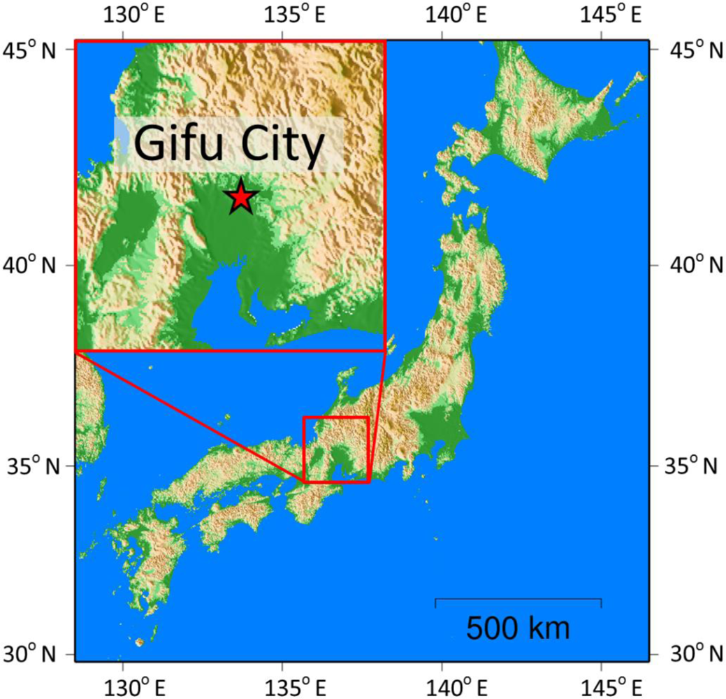
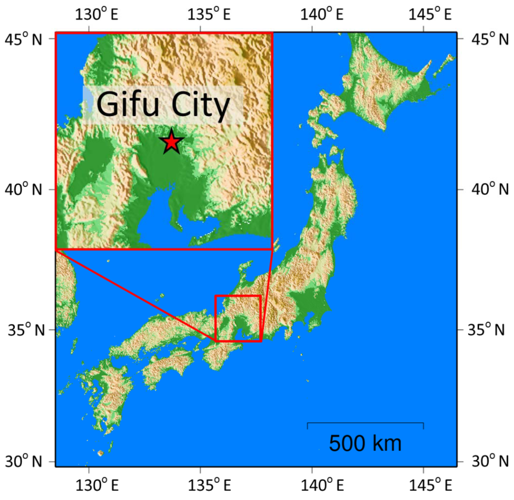
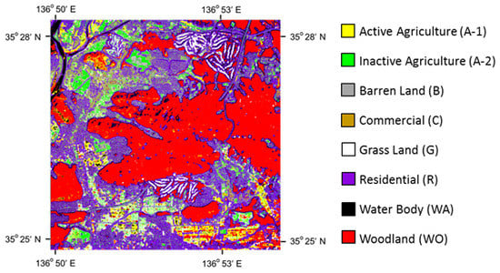
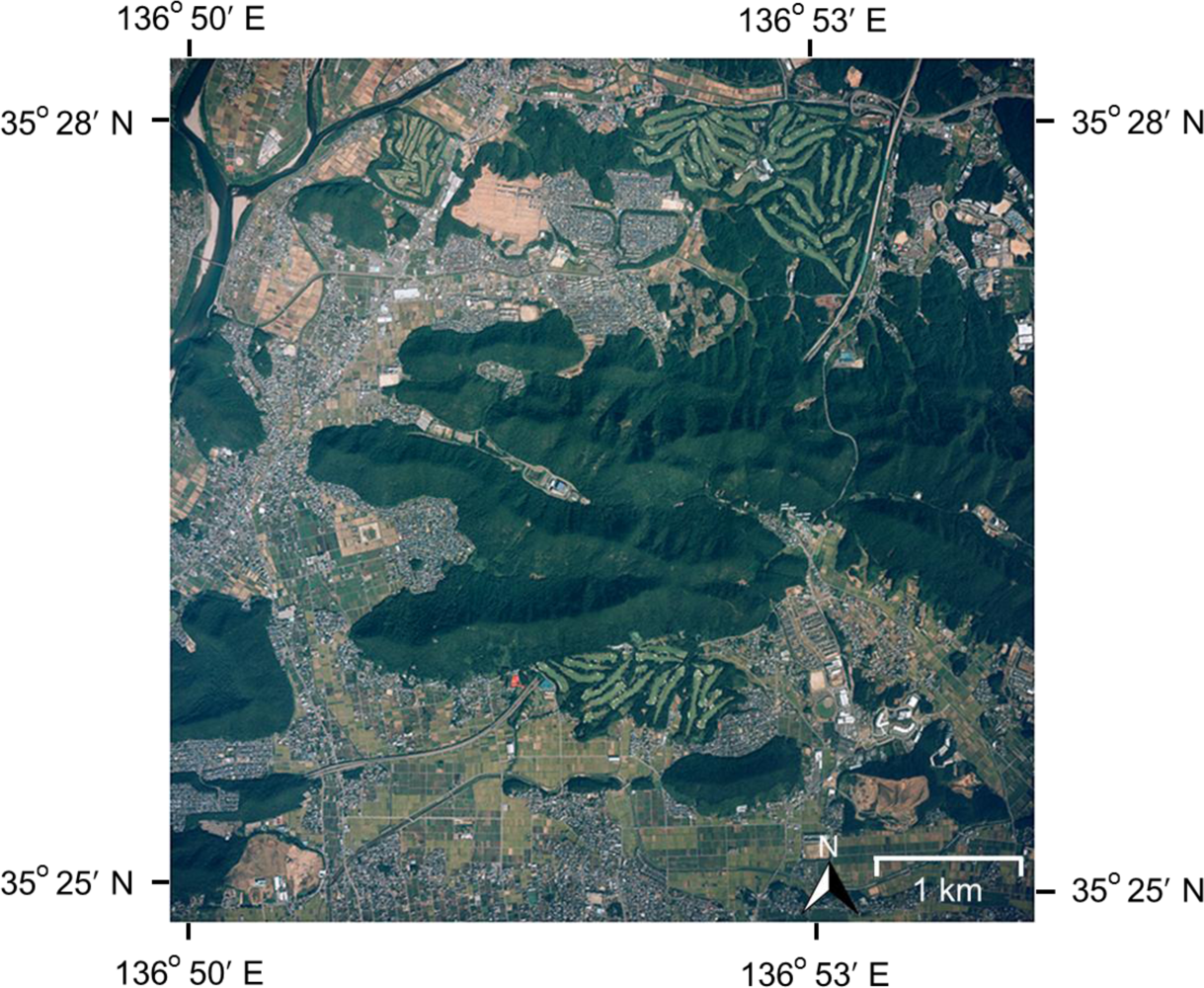
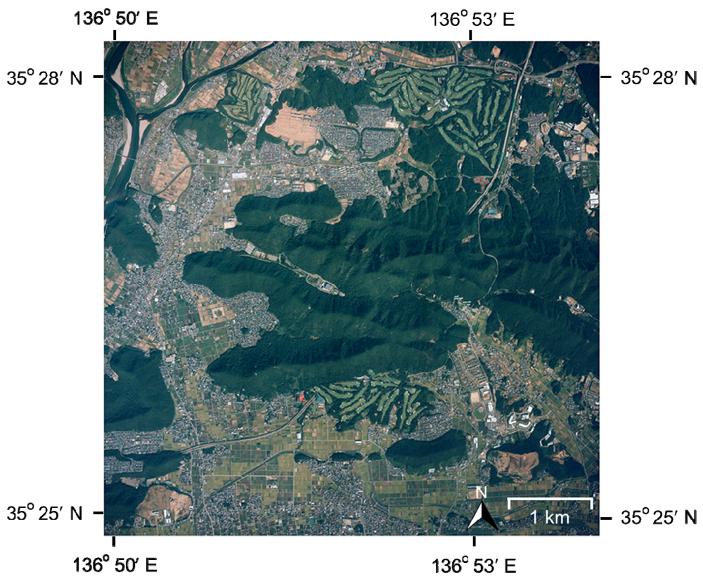
An aerial photo with a 0.3 m spatial resolution was used to identify urban land-use and land-cover categories. The image contains three bands: visible red, visible green, and visible blue. The image was acquired over Gifu City, Gifu Prefecture, Japan on 5 October 2000. The location of the study site is shown in Figure 1. 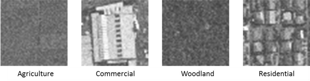A subset of the aerial photography data (4,000 pixels × 4,000 pixels), which contains parts of Gifu City, Kagamihara City, and Seki City, is shown in Figure 2. The original resolution of the aerial photograph was degraded to 1.5 m before beginning the analysis to minimize the analysis time. Gifu City, Kagamihara City, and Seki City offer conditions appropriate for examining the applicability of lacunarity approaches for the identification of complex land-use and land-cover features. There are various land-uses (i.e., agriculture, commercial, residential, barren land, and grass) and land-covers (i.e., water body and woodland) in this study area. This area was also selected for the case study because it includes vegetated and non-vegetated agricultural areas. This variety of land-uses and land-covers is adequate assessing the effectiveness of the classification approaches examined in this study. The area also includes mountains (Gongen Mountains and Kita Mountains). The effectiveness of the lacunarity analysis and gradable approaches for mountainous areas were addressed in this study. The aerial photography was classified into eight categories: Active Agriculture (A-1), Inactive Agriculture (A-2), Barren Land (B), Commercial Land (C), Grass (G) Residential Land (R), Water Body (WA), and Woodland (WO). Here, we recognize urban forest and mountains for trekking as “woodland (WO)”.

3. Methodology

Gradable classification approaches using the brightness values of the original and lacunarity index images are proposed for the classification of land-use and land-cover with high-resolution aerial photographs. The approaches compare different classified-maps in incremental steps to improve the classification accuracy. To assess the applicability of the gradable approaches, we examined the following six types of techniques:

• Approach (S): Classification based on spectral response imaging
• Approach (L): Classification based on lacunarity imaging
• Approach (SL): Classification based on both spectral response and lacunarity imaging
• Approach (G1): Gradable classification applying results of both the (S) and (SL) approaches
• Approach (G2): Gradable classification applying results of both the (L) and (SL) approaches
• Approach (G3): Gradable classification applying results of the (S), (L), and (SL) approaches

The details of each classification approach (S, L, SL, G13) are provided below.

3.1. Basic Information of the S, L and SL Classification Approaches

In the (S), (L), and (SL) approaches, land-use and land-cover were classified by MLC. A supervised classification approach with MLC was employed to identify the classes in the (S), (L), and (SL) approaches. For these classifications (S, L, and SL), we employed the software program GRASS, which offers supervised classification using MLC with multiple-bands. For the supervised classification approach, three to five training data per category were used in previous studies [7,8]. However, the classification results obtained from additional training sets are expected to be better from a statistical point of view. Thus, we extracted 10 training samples, each measuring 5 × 5 pixels, from each class (i.e., the number of training data points was 80). These training data were carefully extracted from an aerial photo by visual inspection. To extract the training samples, we used two reference data: (1) A classified map using the unsupervised classification algorithm and (2) Land Use Fragmented Mesh Data. The unsupervised classification algorithm automatically classified the aerial photo used in this study into the same categories by using MLC technique. The mesh data consisted of a land-use and land-cover map published by Japan’s Ministry of Transport and Tourism. These mesh data were compiled between 1997 and 2006 with a 10 m spatial resolution. To be consistent with all of the approaches used in urban image analysis and to compare the classification accuracies, we used the same training points for the supervised classification approach among the six classifications. Figure 3 shows an example of some of the land-use and land-cover classes. The lacunarity approach used in this study is discussed in detail below.

3.2. Lacunarity Probability Method (L)

3.2.1. Concept of Lacunarity

The concept of lacunarity was introduced by Mandelbrot [15] to describe the distribution of gap sizes in a fractal sequence. Several other algorithms have been developed for the computation of lacunarity [16–21]. Geometric objects appear to be more lacunar if they contain a wide range of gap sizes. As a result, lacunarity can be considered to be a measure of the “gappiness” or “hole-iness” of a geometric structure. Plotnick et al. [24] emphasized the concept and utilization of lacunarity for the characterization of spatial features. Lacunarity methods for urban analysis and many other applications in geospatial research have been reported by a number of researchers [7,8,20,21,25,26]. Lacunarity can be used with both gray-scale data and binary images [27]. Voss [18] proposed a lacunarity probability approach using gray-scale images to estimate the lacunarity value of an image. Myint and Lam [7,8] insisted that the lacunarity approach involving gray-scale images extracts land-use and land-cover more accurately than that involving binary images. Thus, in this study, we applied the lacunarity probability approach using gray-scale images.

Allain and Cloitre [19] presented an algorithm to calculate lacunarity using what they refer to as a “gliding box”, which was employed in this study, using the programming language Ruby. This gliding box is placed over the upper left corner of an image window called the “moving window”. This window moves through the entire area of the image. The lacunarity is calculated for the group of pixels that falls within each window. The algorithm assigns a lacunarity value to the center of the window as it moves through the image. Thus, we obtain a map-assigned lacunarity value in pixels. In this paper, the map is referred to as a “lacunarity map”. The spatial arrangement of the points determines the parameter P(m,L), which is the probability that there are m intensity points (= digital numbers) within an L-sized box that is centered about an arbitrary point in an image. Thus, we have

$$\mathrm{\Sigma }\text{P}(\text{m},\hspace{0.17em}\text{L})=1$$

(1)

Suppose that the total number of points in the image is M. If one overlays the image with boxes of size L, then the number of boxes with m points within the box is (M/m)P(m,L). Thus, we can calculate the first moment M(L) and second moment M²(L) of this distribution as follows:

$$\text{M}(\text{L})=\mathrm{\Sigma }\text{mP}(\text{m},\hspace{0.17em}\text{L})$$

(2)

and

$${\text{M}}^2(\text{L})=\mathrm{\Sigma }{\text{m}}^2\text{P}(\text{m},\hspace{0.17em}\text{L})$$

(3)

Lacunarity can be computed from the same probability distribution P(m,L). Thus, lacunarity Λ (L) is defined as

$$\mathrm{\Lambda }(\text{L})=\frac{{\text{M}}^2(\text{L})-\text{M}{(\text{L})}^2}{\text{M}{(\text{L})}^2}$$

(4)

3.2.2. Determination of the Window and Box Sizes

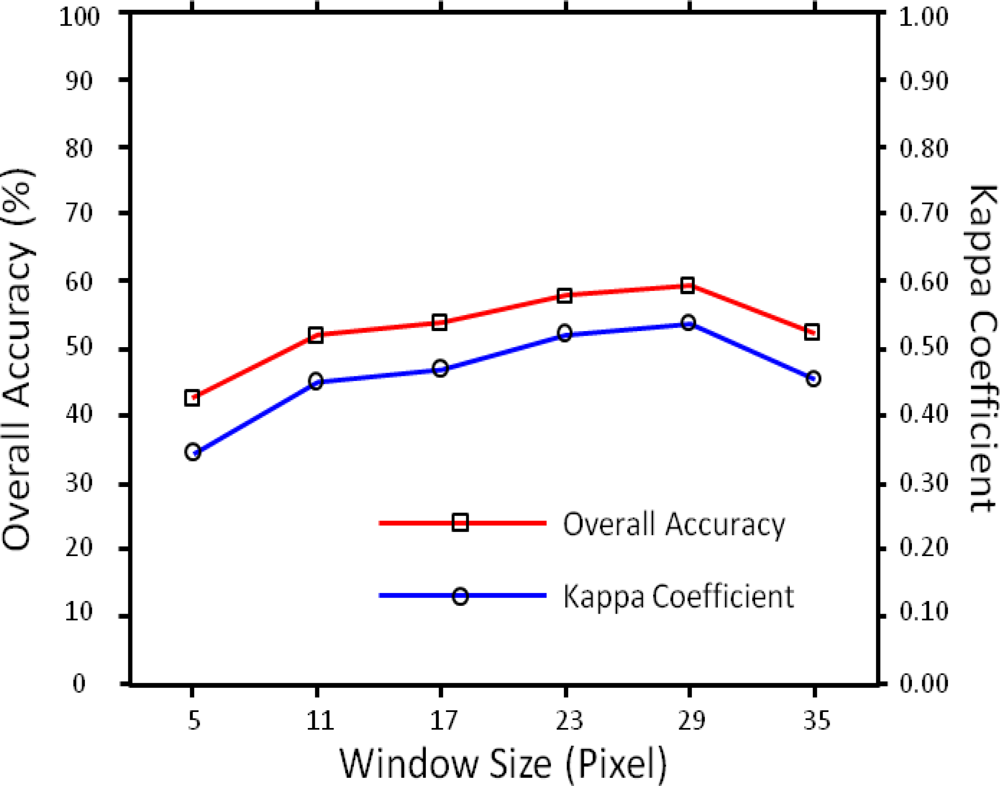
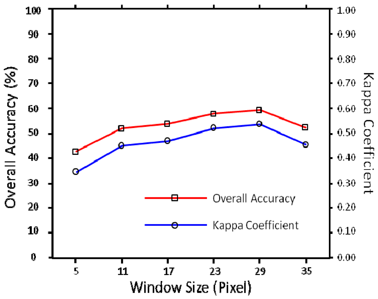
It is often reported that classification accuracy increases with the decreasing size of the box (L = 2–3) used in the lacunarity calculation [7,8,22,28]. Thus, we applied a 2 × 2 box size in this study. However, the appropriate window size also depends on the geographical features of the study site and image resolution. Thus, we examined the supervised classification by the gray-scale lacunarity approach using different local window sizes (i.e., 5 × 5, 11 × 11, 17 × 17, 23 × 23, 29 × 29, and 35 × 35) and assessed the accuracy of the results to determine the optimal window size.

The optimal window size was determined based on the overall accuracy and kappa coefficient of each classified map obtained using each window size. The overall accuracy and kappa coefficient for each classification result are shown in Figure 4. The classification result obtained using a 29 × 29 window provided the highest overall accuracy and kappa coefficient in the lacunarity approaches. Thus, in this study, we used an optimal window size of 29 × 29 for the classification of the land-use and land-cover using the lacunarity method.

3.3. Gradable Classification Method

In this study, we proposed “gradable classification approaches (G1-3)” as new classification approaches for the identification of land-use and land-cover. The gradable approach classifies land-use and land-cover using the classification results of (S), (L), and (SL). Lacunarity should be calculated using an appropriate window size. The optimal window size was determined based on the accuracy of the classification result that was applied using the lacunarity approach with different window sizes. Land-use and land-cover were classified by using three lacunarity maps (termed L), original RGB images (termed S) and combinations of both of them (termed SL). A supervised classification approach using MLC with 80 training data was employed to identify the classes in (S), (L), and (SL).

3.3.1. Concept of the Gradable Classification Method

The details of the gradable classification technique are provided below. Suppose that two classified maps (maps A and B) are divided into “k” categories. Each classified map was classified with a different index (e.g., the digital number of the original image and the lacunarity index). First, we created two error matrices for maps A and B using the same training data (

Table 1. Error matrix for classification map A.

Reference Data
Category	Category 1	· ·	Category k	Row Total
Category 1	A 11	· ·	A 1k	A Row Total 1
:	:		:	:
Category k	A k1	· ·	A kk	A Row Total k
Column Total	100	100	100

and

Table 2. Error matrix for classification map B.

Reference Data
Category	Category 1	· ·	Category k	Row Total
Category 1	B 11	· ·	B 1k	B Row Total 1
:	:		:	:
Category k	B k1	· ·	B kk	B Row Total k
Column Total	100	100	100

). The number of training data per category is the same. In this example, the number of training datasets for each attribute is assumed to be 100.

The gradable method classifies land-use and land-cover using the index for gradable classification (IGC), which is explained below. For instance, one pixel was classified as category α (1 ≤ α ≤ k) in map (A). In contrast, the same pixel was classified as category β (1 ≤ β ≤ k) in map (B). In this situation, the IGC value for the error matrices of maps A and B can be calculated using the following formula, respectively:

$${\text{IGC}}_{(\text{Map}\hspace{0.17em}\text{A})}=\frac{{\text{A}}_{\alpha \alpha }-{\text{A}}_{\alpha \beta }}{{\text{A}}_{\text{Row} \text{Total} \alpha }}$$

(5)

$${\text{IGC}}_{(\text{Map} \text{B})}=\frac{{\text{B}}_{\beta \beta }-{\text{B}}_{\beta \alpha }}{{\text{B}}_{\text{Row} \text{Total} \beta }}$$

(6)

In the gradable classification approach, the category of the classification map with the higher IGC value is applied to the pixel’s attribute.

3.3.2. Example Showing the Gradable Classification Calculations

In this paper, we explain how to calculate the IGC value with an example. Suppose that classified maps A and B are created in an identical manner using the (S) and (L) approaches, respectively. These maps are classified into three categories: forest, urban, and water.

Table 3. Example of error matrix for classification A.

Reference Data
Category	Forest	Urban	Water	Row Total
Forest	5	3	1	9
Urban	2	6	3	11
Water	3	1	6	10
Column Total	10	10	10

and

Table 4. Example of error matrix for classification B.

Reference Data
Category	Forest	Urban	Water	Row Total
Forest	7	2	3	12
Urban	1	6	0	7
Water	2	3	7	12
Column Total	10	10	10

are the error matrices for classified maps A and B, respectively.

Assume that the pixels for the same coordinates are classified as forest and urban in maps A and B, respectively. Gradable classification determines the pixel category by the following calculation:

$${\mathbf{IGC}}_{(\mathbf{Map}\hspace{0.17em}\mathbf{A})}=\frac{5-3}{9}=0.2$$

(7)

$${\mathbf{IGC}}_{(\mathbf{Map}\hspace{0.17em}\mathbf{B})}=\frac{6-1}{7}=0.7$$

(8)

From the result of the calculation, IGC_{(Map A)} < IGC_{(Map B)}; thus, this pixel is categorized as urban. In this study, three options of the gradable classification approach were examined (G1, G2, and G3). G1 applies the results of spectral classification (S) and a hybrid of the spectral and lacunarity (SL) methods. The results of the lacunarity method (L) and hybrid approach (SL) were used in G2. G3 employs the results of (G1) and (L). The classification result of (SL) was used in all of the gradable classifications (G1, G2, and G3) because the accuracy of this result was the highest among the classification results obtained using the (S), (L), and (SL) approaches.

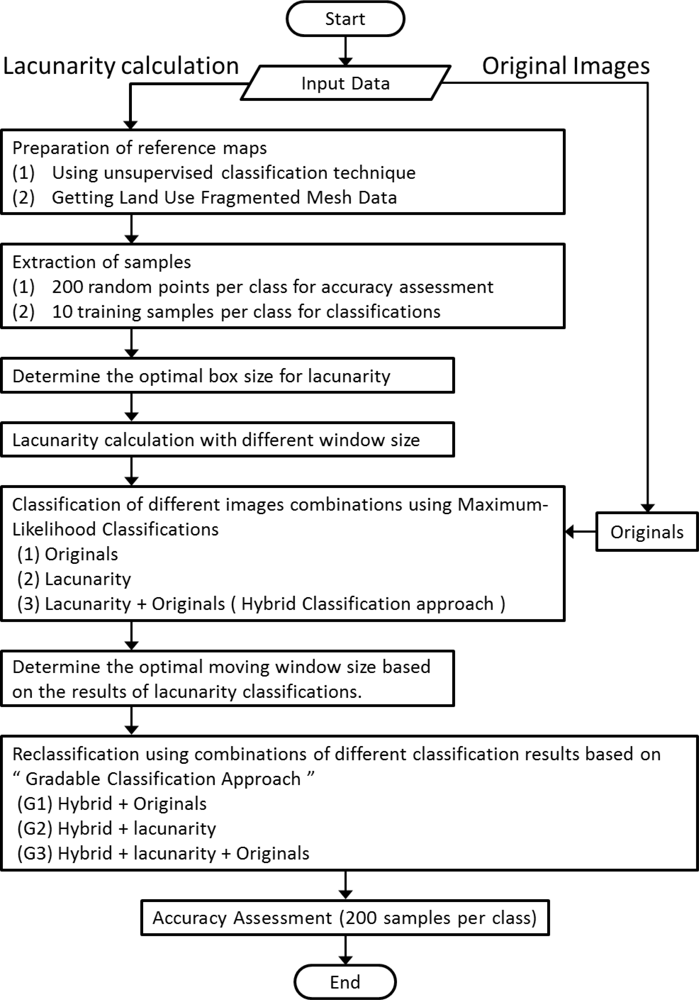
3.4. Accuracy Assessment for the Land-Use and Land-Cover Classifications

In this study, the kappa coefficient [29] and overall accuracy [30] were applied using an error matrix to assess the accuracy of the classifications. The kappa coefficient is an index of the coincidence rate that does not depend on chance. As this value increases, the accuracy of the classifications also increases. To assess the accuracy of the classifications, 200 sample points were extracted from each category using a random sampling technique. The randomly identified sample points were displayed on the original aerial photograph by visual inspecting the aerial photographs. In this step, we used two categorized maps as references: (1) a classified map using the unsupervised classification algorithm and (2) Land Use Fragmented Mesh Data. To be consistent with all of the approaches in the urban image analysis and to compare of the classification accuracies, we used the same sample points to assess the accuracy among the six classifications.

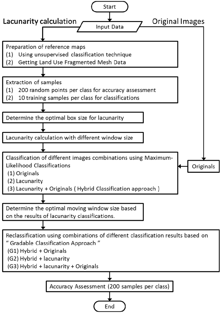
The flow chart of this study is shown in Figure 5.

4. Results and Discussion

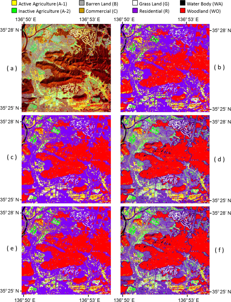
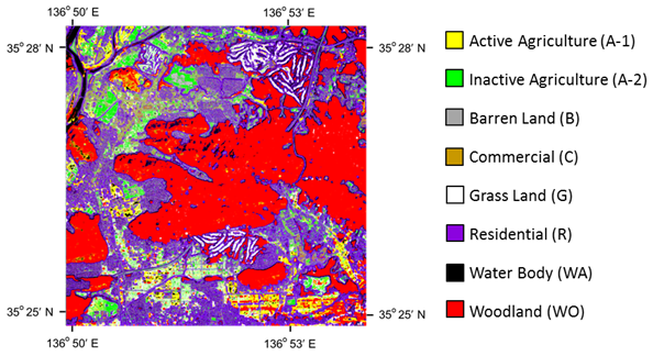
The output maps of the six approaches (i.e., classification techniques S, L, SL, G1, G2, and G3) are shown in Figure 6. From the classified maps, it is confirmed that there are different features among these classification approaches. Approach S recognizes land-use/land-cover on a micro scale. Thus, approach S can even identify very small objects. In contrasts, approach L perceives land-use/land-cover by considering the spatial features of the objects. Thus, the classification map of approach L shows regional land-use/land-cover. One of the main disadvantages of approach L is that the classification accuracy around boundaries between different land-use/land-cover is low because of the characteristics of L. The results of approaches SL and G2 show features similar to those of L. Approaches G1 and G3 show the features of both S and L. Figures 6-(4) and (6) confirm that approaches G1 and G3 discern small objects by considering the spatial features of land-use/land-cover. Moreover, approaches G1 and G3 discern the boundaries between different land-uses/land-covers (i.e., a boundary between residential and woodland).

The results showed that the gradable approach using several classified maps (the results of SL, S and/or L) improves the accuracy of classification when identifying land-use and land-cover with high-resolution image data in urban areas. The classification accuracy of approaches (S), (L), (SL), (G1), (G2), and (G3) are shown in

Table 5. Classification accuracy produced by the (S), (L), (SL), (G1), (G2), and (G3) approaches.

	Classification Approaches
	(S)		(L)		(SL)		(G1)		(G2)		(G3)
Category	Pro Acc	Use Acc	Pro Acc	Use Acc	Pro Acc	Use Acc	Pro Acc	Use Acc	Pro Acc	Use Acc	Pro Acc	Use Acc
A-1	54	39	53	63	65	71	64	71	58	73	57	73
A-2	44	56	55	59	67	67	77	60	68	62	76	59
B	54	50	23	96	28	95	38	60	28	95	36	71
C	64	77	36	44	36	55	66	71	37	57	68	74
G	59	75	63	53	65	62	79	70	62	59	78	67
R	26	34	99	45	100	43	52	49	99	47	57	54
WA	61	47	65	76	68	95	78	80	74	82	83	72
WO	38	33	82	87	91	83	91	83	92	81	92	81
Over Acc		50		59		65		68		64		68
Kappa Co		0.43		0.54		0.60		0.63		0.59		0.64

(S) Classification with per-pixel value; (L) classification by the lacunarity index; (SL) hybrid classification using both per pixel value and lacunarity; (G1) gradable method obtained using the results of (SL) and (S); (G2) gradable method obtained using the results of (SL) and (L); (G3) gradable method obtained using the results of (SL), (S), and (L) methods. Pro Acc = producers accuracy; Use Acc = users accuracy; Ovr Acc = overall accuracy; Kappa Co = Kappa coefficient.

.

Among the six approaches (i.e., methods S, L, SL, G1, G2, and G3), classification technique (G3) displayed the highest overall accuracy and kappa coefficient (overall accuracy = 68%, kappa coefficient = 0.64). Also, the (G1) approach displayed the second-highest accuracy (overall accuracy = 68%, kappa coefficient = 0.63). As mentioned earlier, the spectral response from different land-cover features consisting of urban environments typically exhibits a spatial complexity in high-resolution images. Thus, to identify urban land-use and land-cover classes, we must consider the spatial arrangements of neighborhood features and objects that have textures and patterns, as well as individual pixel values [23]. From this perspective, it was determined that gradable classification is an approach that identifies land-use and land-cover by considering per-pixel spectral data and textural information effectively.

The classification approach (G2) produced an overall accuracy of 64% and a kappa coefficient of 0.59. These accuracies are slightly lower than those of approach (SL), which exhibits an overall accuracy of 65% and a kappa coefficient of 0.60. These results confirm that the combination of images used in the gradable approach is an important factor for classifying land-use and land-cover with high accuracy. An appropriate combination of the applied classification maps should be discussed and surveyed in the future. The output maps from conventional per-pixel image-classification techniques (S), lacunarity approach (L), combination method (SL), and three types of gradable classification methods (G1, G2, and G3) are shown in Figure 6.

As mentioned earlier, we used the same training samples for the supervised classification and the same number of random points for the accuracy assessment.

The features of each classification result are discussed below. The conventional per-pixel classification (S) identified a part of the mountain’s shadow area WA because the pixel values of the river and the shadow of the mountains were similar. In the lacunarity approach (L), the areas shadowed by mountains were accurately classified as woodlands. However, approaches (L) and (G2) misrepresented an A-1 area as R, and the features of the lacunarity classification were also observed in the SL approach. In contrast, G1 and G3 considerably improved these incorrect classifications.

5. Conclusion

In this study, a new concept, referred to as gradable method, for land-use/land-cover classification was proposed. This approach shows an overall accuracy that is 4% higher than that of the conventional hybrid method by using digital numbers and lacunarity in this case. The classification approaches recognize small objects by considering the spatial features of land-use/land-cover. This study also confirmed that the proposed methods improve the boundary problem, which is characterized by the fact that the classification accuracy of the lacunarity approach tends to be low because of lacunarity’s characteristics. Based on the above discussion, it can be safely concluded that the gradable approach can be employed to effectively improve land-use/land-cover classification. From this point of view, the method is expected to improve classification accuracy by using another combination of indices (i.e., Haralick texture parameters [13]). It is also anticipated that using indices that exhibit different features (i.e., spectral responses and structures) will be better in compensating for their disadvantages in gradable approaches. Moreover, the combination of indices should be changed based on the location and aims of future studies. Furthermore, it should be noted that the selection of the local moving window and gliding box sizes (issue of scale) plays an important role in determining the accuracy of characterizing spatial features for land-use and land-cover classification. Thus, future studies should focus on a more in-depth evaluation of window sizes and gliding box sizes and their effects on different types of land-use and land-cover classification.