Article

Discrimination of Switchgrass Cultivars and Nitrogen Treatments Using Pigment Profiles and Hyperspectral Leaf Reflectance Data

1
Department of Plant and Soil Sciences, Oklahoma State University, Stillwater, OK 74078, USA
2
Department of Geography, Oklahoma State University, Stillwater, OK 74078, USA
3
The Samuel Roberts Noble Foundation, Inc., 2510 Sam Noble Parkway, Ardmore, OK 73401, USA
*
Author to whom correspondence should be addressed.
Remote Sens. 2012, 4(9), 2576-2594; https://doi.org/10.3390/rs4092576
Submission received: 18 July 2012 / Revised: 16 August 2012 / Accepted: 28 August 2012 / Published: 10 September 2012

Abstract

:
The objective of this study was to compare the use of hyperspectral narrowbands, hyperspectral narrowband indices and pigment measurements collected from switchgrass leaf as potential tools for discriminating among twelve switchgrass cultivars and five N treatments in one cultivar (Alamo). Hyperspectral reflectance, UV-B absorbing compounds, photosynthetic pigments (chlorophyll a, chlorophyll b and carotenoids) of the uppermost fully expanded leaves were determined at monthly intervals from May to September. Leaf hyperspectral data was collected using ASD FieldSpec FR spectroradiometer (350–2,500 nm). Discrimination of the cultivars and N treatments were determined based on Principal Component Analysis (PCA) and linear discriminant analysis (DA). The stepwise discriminant analysis was used to determine the best indices that differentiate switchgrass cultivars and nitrogen treatments. Results of PCA showed 62% of the variability could be explained in PC1 dominated by middle infrared wavebands, over 20% in PC2 dominated by near infrared wavebands and just over 10% in PC3 dominated by green wavebands for separating both cultivars and N treatments. Discriminating among the cultivars resulted in an overall accuracy of 81% with the first five PCs in the month of September, but was less accurate (27%) in classifying N treatments using the spectral data. Discrimination based on pigment data using the first two PCs resulted in an overall accuracy of less than 10% for separating switchgrass cultivars, but was more accurate (47%) in grouping N treatments. The plant senescence ratio index (PSRI) was found to be the best index for separating the cultivars late in the season, while the transform chlorophyll absorption ratio index (TCARI) was best for separating the N treatments. Leaf spectra data was found to be more useful than pigment data for the discrimination of switchgrass cultivars, particularly late in the growing season.

1. Introduction

Switchgrass (Panicum virgatum L.), a native North American warm-season C4 perennial grass has been identified as a potential biofuel feedstock with a promise for production across diverse climates in North America [13]. Switchgrass is adapted to a wide range of climatic and edaphic conditions from northern Mexico to southern Canada, and from the Atlantic coast to the Rocky Mountains [3]. It is classified as a dedicated biofuel feedstock due to its high level of productivity over long-term (>10 yr) across varied environmental conditions [4], suitability for production on marginal land [3], low nutrient requirements [1,5], and positive environmental benefits such as reduced erosion, increased water quality, enhanced soil-carbon sequestration, wildlife habitat and reducing greenhouse gas emissions [2].
Two major types of switchgrass are found in North America: the low land ecotype is exclusively tetraploid, associated with wet conditions and better adapted to lower latitudes, while the upland ecotype is mainly tetraploid or octaploid, associated with dry conditions and better adapted for mid to northern latitudes [6,7]. Because of these distinct differences between and within the upland and lowland ecotypes, it is important to be able to discriminate switchgrass plants. Current methods of identification of specific cultivars are limited to genomic analysis and visual discrimination. Despite genomics analysis only requiring a small amount of sample material, expensive equipment and expertise are needed to make the assessment. While, visual discrimination is possible with trained personnel, results among personnel and locations can vary due to plants of different age and localized effect of light, temperature and moisture.
Remote sensing is a well-known non-destructive method that can play a critical role as a crop stress assessment tool, monitoring nutrient status, disease and weed and insect infestation. The basic concept of remote sensing is the ability to quantify variations due to space and size (spatial variations), variations in reflected or emitted radiation (spectral variations) and variations of reflected or emitted radiation, space and size over time (temporal variations) [8]. Radiation reflected by vegetation varies in different part of the spectrum due to the vegetation biophysical characteristics. In the visible part of the spectrum (400–700 nm) the amount of reflected or emitted radiation is controlled by the plant pigmentation the chlorophyll, carotenes and xanthophylls [8]. In the near infrared portion of the spectrum (700–1,350 nm) reflected or emitted radiation is controlled by the internal leaf structures. The middle infrared (Mid-IR) portion of the spectrum (1,350–2,500 nm) reflected or emitted radiation is controlled primarily by in vivo water content and secondarily by internal leaf structures [8]. The importance of these parts of the spectrum (Mid-IR) is the high resolution spectral response that is often observed for a crop at leaf or canopy level at different stages of development. As a plant develops and interacts with environmental conditions, reflectance from these areas of the spectrum is affected. Reflectance tends to increase in the near-infrared (NIR; 725–900 nm) as the internal leaf structure of most plant species (i.e., cotton canopy) reflects more of the energy in this portion, and changes in green peak (550 nm) and in red region (650–690 nm) due to chlorophyll reflectance and adsorption respectively [9].
The recent advances in ground-based high resolution multispectral, hyperspectral digital cameras, spectroradiometers and several other optical sensors can play a critical role towards a more intelligent crop production system. Narrowbands located in specific portions of the spectrum have been shown to significantly improve discrimination capabilities and classification accuracies for various vegetation and agricultural crops when compared to broadbands such as Landsat Thematic Mapper ™ and Systeme Pour L’Observation de la Terre (SPOT) [10]. Hyperspectral narrowbands and vegetative indices developed from them are capable of detecting small differences in percentage green cover [11], crop moisture variations [12] and discriminating among varieties [13,14]. Despite, the improvement of narrowbands over broadband, the large number of bands available with hyperspectral sensors makes analysis complex and time consuming [14]. Several approaches were used including reflectance from individual narrowbands, various ratios and indices, and multivariate statistical analysis to discriminate among varieties. The use of high resolution hyperspectral leaf reflectance with pigment profiles to discriminate among sugarcane varieties was investigated [13]. The hyperspectral reflectance data was collected at 350–800 nm at 0.4 nm intervals from the third youngest fully open leaf and plant pigment analysis was done from the same leaf. The authors reported that several single wavelengths ranging from 560 to 720 nm were able to discriminate between selected varieties, multivariate analysis resulted in a 95–100% correct classification for all varieties with leaf reflectance data in comparison to 76–81% correct classification with plant pigment data and 81–86% using vegetative indices [NDVI (Normalize Difference Vegetative Index) and WDRVI (Wide Dynamic Range Vegetative Index)]. Hyperspectral narrowband wavelengths from 375 to 1,075 nm and multiple discriminant analysis were used by Ray et al. [14] to identify nine bands (520, 560, 660, 690, 730, 760, 780, 790 and 800 nm) and vegetative indices, simple ratio, ZTM (Zarco Tejada and Miller), Red edge 750/700 and Red edge 740/720 for discriminating among four potato varieties. Likewise, Hatfield and Prueger [15] used different vegetative indices to quantify differences among varieties of corn and soybean at different growth stages during the growing season. The authors concluded that the ability to quantify differences among the varieties and crops was a function of growth stage and vegetative index.
The use of hyperspectral remote sensing techniques, with high spectral resolutions, in combination with plant pigment analysis may significantly improve the ability to discriminate between and among switchgrass cultivars and ecotypes. The dominant plant pigments are the chlorophylls. These compounds exhibit pronounced absorption in the bluish (400–500 nm) and reddish (600–700 nm) wavelengths of the magnetic spectrum. Other plant pigments such as carotenoids produces yellow or orange reflectance centered at about 450 nm wavelength of the spectrum. Knowledge of pigment pools including those associated with UV-B absorption could improve our understanding of plant stress responses to light, temperature and water, and could also be used to discriminate between species, cultivars and varieties of switchgrass. The objective of this study was to compare the use of hyperspectral narrowbands, hyperspectral narrowband vegetation indices and leaf pigmentation (Chlorophyll a, Chlorophyll b, Carotenoids) to discriminate between 12 switchgrass cultivars and five nitrogen treatments for one of the cultivars (Alamo) at different times during the growing season.

2. Materials and Methods

2.1. Experimental Design

2.1.1. Switchgrass Cultivars

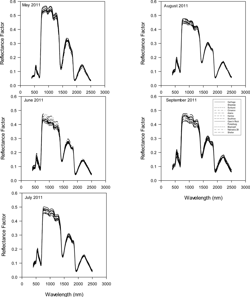
An experiment consisting of twelve cultivars of switchgrass (Figure 1) with known difference in ecotype, and origin (Table 1) was established at the Stillwater Agronomy Research Station (36.12°N, 97.09°W) in April 2009 to evaluate biomass yield production among the cultivars. Switchgrass cultivars were planted by seed in plots (6.10 m wide × 7.62 m long) in a randomized complete block design with three replications. Plots were seeded at a rate of 5.04 kg·ha−1 of pure live seed using a no-till planter. Leaf samples were collected on 24 May, 20 June, 25 July, 24 August and 30 September 2011 from which the spectral and pigment data was obtained (Table 2).

2.1.2. Nitrogen Treatments

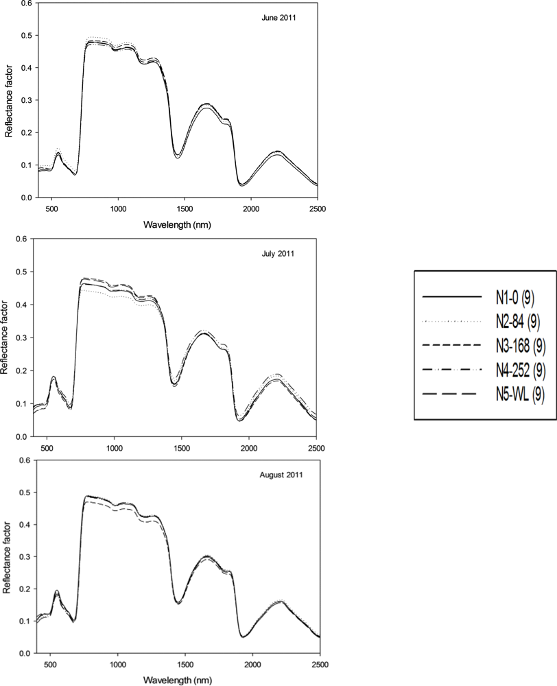
An experiment consisting of five nitrogen treatments (winter legume (hairy vetch), 0, 84, 168 and 252 kg·N·ha−1) was established at the Stillwater Agronomy Research Station (EFAW Site, 36.13°N, 97.10°W) in a one year old established stand of switchgrass “Alamo” to evaluate the effect of nitrogen treatment on biomass production. Experimental design is a randomized complete block and replicated three times. No nitrogen fertilizer was applied in the establishment year. Plots were fertilized with the different rates of N on 3 June 2011. Leaf samples were collected on 17 June, 27 July and 27 August 2011 from which the spectral and pigment data was obtained (Table 2).

2.2. Leaf Sampling

Top most fully expanded leaf (6th or 5th) was excised from 6 random plants in each plot and sealed in a plastic bag in an ice chest and transported to the laboratory for spectral and pigment measurements. These samples were collected between 10:00 and 15:00 h local time.

2.3. Spectral Data

Hyperspectral reflectance data was collected using an ASD Field Spec Pro spectroradiometer (Analytical Spectral Devices Inc., Boulder, CO, USA) that consisted of a spectral range of 350–2,500 nm and a 25° field of view. The spectrometer is equipped with three sensors [(visible (400–750 nm) and near infrared-NIR (750–1,100 nm), shortwave infrared-SWIR1 (1,000–1,800 nm) and SWIR2 (1,800–2,500 nm)] with spectral sampling of 3, 10 and 10 nm, respectively. The instrument was periodically calibrated using a standard Spectralon white reference panel (Labsphere Inc., North Sutton, NH, USA). The white reference was measured at 15 min intervals to check the instrument stability for 100% reflectance. To measure leaf reflectance, two leaves were place beside each other to provide a large enough surface area, and sandwiched between the non-reflecting, black body and the light probe. This ensured that no extraneous light entered the sensor during these measurements. Care was taken in placing the leaves beside each other, to ensure that no space or overlapping occurred. Three replicated measurements were made on leaves collected from each plot. Built-in spectral resolution output of the data from the ASD operating system is 1 nm along the whole spectrum. To reduce the amount of data for analysis, spectral data were averaged at 10-nm wavelength intervals (e.g., a band center at 400 was the averaged value between 395–405 nm) giving a total of 211 spectral bands between 400–2,500 nm. Spectral data at start of spectrum due to noise (350–395 nm) and in the atmospheric water absorption spectral regions (1,350–1,420 and 1,800–1,960 nm) were deleted from the data before analysis leaving 186 spectral bands for analysis.

2.4. Pigment Analysis

After reflectance measurements, five of the leaves used for hyperspectral measurements were sampled for plant pigment analysis. The photosynthetic pigments (Chlorophyll a, Chlorophyll b and Carotenoids) were extracted by placing five 38.5 mm2 leaf discs in a vial with 5 mL of dimethyl sulfoxide and extracting after incubating in a dark room for 24 h. The absorption of the extracts was determined at 664, 648 and 470 nm using the spectrophotometer. The equations by Lichtenthaler [16] were used to derive the pigment concentrations.
The UV-B absorbing compounds were determined using methods described in Kakani et al. [17]. UV-B absorbing compounds were extracted from placing five 38.5 mm2 leaf discs in a vial with 10 mL of aliquot consisting of a methanol, water and hydrochloric acid in the proportion of 79:20:1 ratio. The vials were incubated at room temperature for 24 h in dark to allow for complete extraction of UV-B absorbing compounds. The absorbance of the extracts from the different cultivars was measured at 330 nm. The content of UV-B absorbing compounds was calculated using the equation [17], C = 16.05 × A, where A is absorbance at 330 nm and C is concentration of UV-B absorbing compound (μg·mL−1 of extract).

2.5. Data Analysis

The optimal wavebands that were able to discriminate the target as affected by time of collection were determined based on a comprehensive analysis using principal component analysis (PCA). The goal of the PCA is to identify underlying variables, or factors that explain the pattern of correlations within a set of observed variables. The PCA tends to achieve this by deriving a new set of uncorrelated variables called principal components, thereby reducing the number of variables. The PCA was carried out using the PRINCOMP procedure in SAS [18].
To evaluate the effect of time of collection in differentiating among the cultivars and N treatments a linear discriminant analysis with cross validation was done for each month. Discriminant function analysis (DA) is a qualitative tool often used to discriminate between two or more groups. To classify observations into a group, a mathematical rule or discriminant function is used to determine to which group an observation belongs based on knowledge of the quantitative variables only. In this study, DA was used to classify the twelve cultivars and five N treatments, by computing a sample’s distance from each class center in Mahalanobis distance (MD) units [19]. The MD is the parameter that is calculated and used to determine how close to the center of its group is an individual spectrum sample. The MD was calculated using the following equation [19]:
D i j 2 = [ A v ( x i ) A v ( x j ) ] co v 1 [ A v ( x i ) A v ( x j ) ]
where D i j 2 denotes the MD between the cultivars i and j, cov1denotes the inverse covariance matrix, and Av(xi) and Av(xi) denote the mean reflection for cultivars i and j, respectively. The smallest MD is used to pick the group that the individual fits best. The equation assumes a common variance for the populations from which the groups are derived. Discriminant function analysis was carried out on the first five PCAs resulting from the PCA as they covered most of the variation (99% of variation explained) contained in the raw spectral data.
Selected hyperspectral narrowband vegetation indices that take into account leaf structure, pigmentation and red edge characteristics were computed for each set of spectral data. The vegetation indices computed are shown in Table 3. Stepwise discriminant analysis (SDA) was carried out to find the best indices which can differentiate switchgrass cultivars and nitrogen treatments at each sampling interval. The SDA is a procedure that reduces the data set to those variables that maximize between statistical group variability while minimizing within group variability. The difference between PCA and SDA is that the PCA creates a new set of uncorrelated variables that defines the axes of greatest variability in the data, while SDA identifies from among the original variables, the best variables that describes differences between given groups. The Wilk’s lambda statistics was used to select the best vegetation indices for differentiating the cultivars and N treatments. Low Wilk’s Lambda valve suggests a great degree of separation. Therefore, index with the lowest Wilk’s lambda value resulted in the greatest separation among the cultivars and N treatments.
Similarly, PCA and DA were performed at each sampling date for the pigment content to determine degree of discrimination. Discriminant analysis was carried out on the two first PCAs as they contain most of the variation (99% of variation explained). The results were compared to determine the approach and the sampling interval that provided the greatest separation. All statistical analyses were performed using SAS (Statistical Analysis System) [18].

3. Results

3.1. Principal Component Analysis

It is evident from Figure 1 that there was a difference in reflectance at the different sampling dates and among the cultivars. Clear varietal and sampling interval differences were visible in reflectance in almost all the regions of the spectrum. The most distinct differences among the cultivars were observed for the June and September sampling date in the visible, near infrared and early short-wave infrared regions of the spectrum (Figure 2). Small differences in reflectance were also observed in the different regions of the spectrum for the nitrogen treatments (Figure 3). Similar to the cultivars, the most distinct differences were observed in the visible, near infrared and early short-wave infrared regions of the spectrum. In general, reflectance showed an increasing trend with time throughout the growing season. However, to quantify the wavebands having the greatest influence on separating the cultivars and nitrogen treatments at the different sampling dates, principal component analysis was used to reduce the 186 wavebands hyperspectral data to a few bands that explain most of the variability. The first three principal components (Eigen values greater than 1) explained 93–97% of the variability for the five collection months. Therefore, to explain more than 90% of the variability, the 186 wavebands can be reduced to two to three new principal components wavebands (PC1 to PC3). Table 4 provides the five wavebands with the highest factor loading for each principal components resulting in 15 bands in three different regions of the spectrum. The order in which the bands are listed in Table 4 indicates the magnitude or ranking for that band based on its factor loadings. Therefore, for PC1 waveband centered at 1,670 has the highest factor loading followed by 1,660, 1,680, 1,690 and 1,700 nm.
The PC1 was dominated by the middle infrared (Mid-IR) bands explaining 63% of the variability, PC2 by middle infrared (Mid-IR) bands explaining 22% of the variability, and PC3 by the red region of the spectrum explaining 11% of the variability for the switchgrass cultivars. Similarly, PC1 for nitrogen treatments was dominated by Mid-IR bands explaining 53% of the variability, PC2 by NIR bands explaining 29% of the variability (Table 4). However, PC3 was dominated by green bands explaining 14% of the variability.
The result of the principal component analysis of the pigment profiles showed that over 98% of the variability could be explained using the first two principal components. Table 5 summarizes the result of the PCA for the pigment profiles. The PC1 was dominated equally by total chlorophyll and carotenoid concentrations explaining 70 and 72% of the variability and PC2 by phenolics compounds concentration explaining 29 and 27% of the variability for switchgrass cultivars and nitrogen treatments respectively. Photosynthetic pigments were better able to discriminate among the cultivars and N treatments than UV-B absorbing compounds.

3.2. Discriminant Analysis

Discriminant analysis of the first five PC of the spectral data resulted in an overall classification accuracy of 14, 14, 3, 3 and 81% with cross-validation for data collected in the months of May, June, July, August and September respectively, for switchgrass cultivars. In contrast, DA of the pigment data resulted in an overall classification accuracy of 6, 0, 23, 17 and 11% with cross-validation for the five collection dates in chronological order. The greatest difficulty was in classifying Kanlow (44%) which was misclassified as either Southlow or Cimarron. Cultivars Sunburst, Alamo, Southlow and Nebraska 28 were classified with 67% accuracy into the correct group. Carthage, Shawnee, Cave-In-Rock, Forestburg, Blackwell and Shelter were classified with 100% accuracy into the correct group. Contrary to the switchgrass cultivars, classification of the N treatment based on pigment data was 20% greater than spectral data. Classification of nitrogen treatment based on spectral data ranges from 7 to 27% at the different sampling dates. The most accurate classification was achieved in the August sampling. While, classification of N treatments based on pigment data ranged from 7 to 47% for the different sampling dates. Likewise, the most accurate classification was achieved in the August sampling. These results indicate that the accuracy of discriminating among the twelve switchgrass cultivars and five N treatments was highest towards the end of the growing season. It must be pointed out, that it was clear from the charts in Figure 2 and 3 that there was little difference among N treatments and clear difference in the month of September for the cultivars. Therefore, the statistical analysis substantiates what can be deduced from those figures. The inability to discriminate among the five N treatments could be attributed to late application of the N in early June at the time when switchgrass cultivars were over 1.2 m tall compounded with the severe drought condition experienced during the 2011 growing season in Oklahoma. Response of switchgrass grown for biomass to N fertilization has been reported in studies across the USA [3436]. Thomason et al. [35] found limited response to N with N rate up to 448 kg·N·ha1 in Oklahoma and Vogel et al. [36] and Lemus et al. [34]reported switchgrass response to N fertilization to be dependent on location.

3.3. Selection of the Best Vegetation Indices

Stepwise discriminant analysis was carried out to identify the best indices at each sampling interval, from the list of indices in Table 3, for discrimination. The results of the SDA for the twelve switchgrass cultivars showed the optimal Wilk’s lambda values were achieved with different indices at each sampling intervals. The values of Wilk’s lambda were indicative of discriminatory power of the vegetation indices, with the lesser the Wilk’s lambda the greater the degree of differentiation between the cultivars and nitrogen treatments. The optimal Wilk’s lambda values were achieved using two (0.184), one (0.564) and thirteen (0.000) vegetation indices for sampling intervals in June, July and September, respectively, in differentiating the twelve switchgrass cultivars and with one (0.443), four (0.024) and two (0.12) vegetation indices for sampling interval June, July and August, respectively, for the five N treatments. The Wilk’s lambda was lowest for the months of September and July for switchgrass cultivars and N treatments, again indicating that sampling interval was critical in discriminating among the twelve switchgrass cultivars and N treatments. The Wilk’s lambda for the model with only PSRI (0.050) in the month of September was relatively smaller in comparison to the overall Wilk’s lambda for the models at the other sampling intervals. Therefore, PSRI was found to be the best indices and the month of September the best time for data collection for discriminating among the twelve cultivars. For nitrogen, the lowest Wilk’s lambda was achieved for the July sampling with TCARI, MCARI, SIPI, EVI, in the model. The Wilk’s lambda with only the TCARI (0.250) in the model for the month of August was smaller in comparison to Wilk’s lambda for June with TVI. These results indicate that TCARI was the best index and the month of July was the best time for data collection for discriminating among the five N treatments.

4. Discussion

Optimal wavebands are those bands that have the least correlation among them, high information content and are able to discriminate the target. Currently there is no best approach available to determine the optimal number of bands required to discriminate vegetation characteristics [10]. Researchers in the past have used various approaches from incorporating reflectance from individual narrowbands, various indices derivatives of reflectance spectra, or combinations of these. Using discriminant analysis of reflectance data resulted with correctly grouping the twelve cultivars into their respective grouping with an accuracy of 80% using cross-validation and 100% using re-substitution methods for the September sampling. Pigment data was unable to discriminate among the cultivars. However, in discriminating among N treatments pigment data was found to be better than the spectral data. Likewise, Johnson et al. [13] found greater accuracy (95–100%) in classifying sugarcane varieties with leaf spectral reflectance data in comparison to 76–81% accuracy with plant pigment data. The ability to use spectral reflectance data obtained from a spectroradiometer to discriminate or identify plant varieties or cultivars is based on the leaf spectral characteristics that are related to the leaf pigment profile and structure. The leaf spectral characteristics of plants is affected by many factors such as plant species, leaf maturity, microclimate position of the leaf on the plant [37], environmental condition in which plant is grown and time of data collection. The amount of light reflected, absorbed or transmitted in the visible (400–700 nm), near infrared (700–1,350 nm) and middle-infrared (1,350–2,500 nm) is primarily controlled by the leaf pigment profile, internal leaf structure, and in vivo water content respectively [8]. The PCA found middle infrared to be the dominant waveband for PC1 explaining 63% of the variability, NIR wavebands in May and September, and middle infrared wavebands in June, July and August to be the dominant wavebands for PC2 explaining 22% variability and red wavebands in May, July and August and green wavebands in June and September for PC3 explaining 11% of the variability. Thenkabail et al. [10] also found middle infrared wavebands to be the dominant waveband for PC 1 and accounting for a similar 62% of the variability. The middle infrared region of the spectrum dominated the PC1 with a 63% frequency of occurrence suggests that in vivo water content within leaf was the dominant characteristic for discriminating among the cultivars.
The information generated from vegetation indices depends upon the phenological stage and plant parameter to which the index is most closely related [15]. This study identified SDA models with different vegetation indices for discriminating among the cultivars at different sampling intervals, Chlorophyll red edge index and EVI in June, red edge ratio in July and PSRI in September, which is indicative of an index influenced by the phenological or plant parameter to which it is most closely related. The PSRI an index proposed to be sensitive to the senescence phase of plant development had the lowest Wilk’s lambda value in differentiating among the cultivars. This index was most sensitive to the senescence phase in being able to discriminate among the cultivars at leaf level. The PSRI defined as (Red660 − Green510)/NIR760, takes advantage of the reflectance relationships in red, green and near infrared regions of the spectrum [15]. The relatively large Wilk’s lambda value also suggests that the degree of separation was poor in the months of June and July. The low accuracy in classifying the cultivars during these months confirms this. Furthermore, chlorophyll/pigment related indices that most closely match to the leaf chlorophyll content were most dominant in discriminating among the N treatments. Nitrogen concentration in green plants is related to chlorophyll content [38]. Studies have shown that leaf chlorophyll content can indicate N stress in corn [39], rice [40,41], and sorghum [42]. The indices identified that discriminated among the N treatments were dominated by chlorophyll/pigment related computed indices (SIPI, MCARI and TCARI), again showing relation to the parameter the index is most closely related. TCARI an index that is sensitive to changes in chlorophyll concentrations takes advantage of the reflectance relationships in the red, red edge and green regions of the spectrum occurred in both July and August model for discrimination. The dominant plant pigments were the chlorophyll and carotenoids explaining over 70% of the variability in PC1 (Table 4). In general, chlorophyll reflectance and absorption is associated with a green peak (∼550 nm) followed by a decrease in red reflectance (∼650–690 nm). High spectral resolution measurements of chlorophyll in the red edge region (700–795 nm) was found to detect trace quantities of green vegetation [43]. A leaf simulated reflectance analysis using PROSPECT model was conducted by Haboudane et al. [38]. They reported a negative correlation between TCARI and chlorophyll concentration over a range of (10–70 μg/cm2), and a positive one at concentration below 10 μg/cm2. This indicates that TCARI is highly sensitive to low concentration of chlorophyll.

5. Conclusions

Hyperspectral narrowbands leaf reflectance was able to better discriminate among switchgrass cultivars with 80% accuracy in the month of September in comparison to pigment data. Separation of the nitrogen treatments was more difficult from leaf reflectance data (27% correct classification) than with leaf pigment data (47% correct classification) for the month of August. Hyperspectral narrowbands indices that take leaf structure into account were found to be most dominant in discriminating the cultivars, while chlorophyll pigment based indices were most dominant for the N treatments. The result showed greater success in separating the cultivars using leaf spectral data close to the end of the growing season or harvesting. This finding could be beneficial in development of prediction models for estimating biomass yield for the different cultivars. However, the real benefit in discriminating among cultivars is the ability to discriminate at canopy level in the field. The use of non-destructive techniques to discriminate among cultivars and N treatments at field level could provide an opportunity to evaluate cultivar performance with more detailed genomic or production yield studies and N management in real time. Additional research work is required to determine the ability to discriminate among switchgrass cultivars at canopy level.

Acknowledgments

This study was funded by USDA-NIFA through the Biomass Research and Development Initiative (BRDI), a joint effort between the US Department of Agriculture (USDA) and the US Department of Energy (DOE). This manuscript is a contribution of the Oklahoma Agricultural Experiment Station, Oklahoma State University, Stillwater, OK, USA.

References

  1. Parrish, D.J.; Fike, J.H. The biology and agronomy of switchgrass for biofuels. Crit. Rev. Plant Sci 2005, 24, 423–459. [Google Scholar]
  2. Sanderson, M.A.; Reed, R.L.; McLaughlin, S.B.; Wullschleger, S.D.; Conger, B.V.; Parrish, D.J.; Wolf, D.D.; Taliaferro, C.; Hopkins, A.A.; Ocumpaugh, W.R.; et al. Switchgrass as a sustainable bioenergy crop. Bioresour. Technol 1996, 56, 83–93. [Google Scholar]
  3. Wullschleger, S.D.; Davis, E.B.; Borsuk, M.E.; Gunderson, C.A.; Lynd, L.R. Biomass production in Switchgrass across the United States: Database description and determinants of yield. Agron. J 2010, 102, 1158–1168. [Google Scholar]
  4. Fike, J.H.; Parrish, D.J.; Wolf, D.D.; Balasko, J.A.; Green, J.T.; Rasnake, M.; Reynolds, J.H. Long-term yield potential of switchgrass-for-biofuel systems. Biomass Bioenerg 2006, 30, 198–206. [Google Scholar]
  5. Muir, J.P.; Sanderson, M.A.; Ocumpaugh, W.R.; Jones, R.M.; Reed, R.L. Biomass production of ‘Alamo’ switchgrass in response to nitrogen, phosphorus, and row spacing. Agron. J 2001, 93, 896–901. [Google Scholar]
  6. Cassida, K.A.; Muir, J.P.; Hussey, M.A.; Read, J.C.; Venuto, B.C.; Ocumpaugh, W.R. Biomass yield and stand characteristics of switchgrass in south central US environments. Crop Sci 2005, 45, 673–681. [Google Scholar]
  7. Parrish, D.J.; Fike, J.H.; Bransby, D.I.; Samson, R. Establishing and managing switchgrass as an energy crop. Forage Grazinglands 2008. [Google Scholar] [CrossRef]
  8. Lusch, D.P. Introduction to Environmental Remote Sensing; Center for Remote Sensing and GIS Michigan State University: East Lansing, MI, USA, 1999. [Google Scholar]
  9. Barnes, E.M.; Moran, M.S.; Pinter, P.J., Jr.; Clarke, T.R. Multispectral Remote Sensing and Site-Specific Agriculture: Examples of Current Technology and Future Possibilities. Proceedings of the International Conference on Precision Agriculture, Minneapolis, MN, USA, 23 June 1996; 843–854. [Google Scholar]
  10. Thenkabail, P.S.; Enclona, E.A.; Ashton, M.S.; van der Meer, B. Accuracy assessments of hyperspectral waveband performance for vegetation analysis applications. Remote Sens. Environ 2004, 91, 354–376. [Google Scholar]
  11. McGwire, K.; Minor, T.; Fenstermaker, L. Hyperspectral mixture modeling for quantifying sparse vegetation cover in arid environments. Remote Sens. Environ 2000, 72, 360–374. [Google Scholar]
  12. Penuelas, J.; Gamon, J.A.; Fredeen, A.L.; Merino, J.; Field, C.B. Reflectance indices associated with physiological changes in nitrogen- and water-limited sunflower leaves. Remote Sens. Environ 1994, 48, 135–146. [Google Scholar]
  13. Johnson, R.M.; Viator, R.P.; Veremis, J.C.; Richard, P.E.; Zimba, P.V. Discrimination of sugarcane varieties with pigment profiles and high resolution, hyperspectral leaf reflectance data. J. Am. Soc. Sugar Cane Technol 2008, 28, 63–75. [Google Scholar]
  14. Ray, S.S.; Singh, J.P.; Panigrahy, S. Use of hyperspectral remote sensing data for crop stress detection: Ground-based studies. Int. Arch. Photogramm. Remote Sens. Spat. Inf. Sci 2010, 38, 562–567. [Google Scholar]
  15. Hatfield, J.L.; Prueger, J.H. Value of using different vegetative indices to quantify agricultural crop characteristics at different growth stages under varying management practices. Remote Sens 2010, 2, 562–578. [Google Scholar]
  16. Lichtenthaler, H.K. Chlorophylls and carotenoids-pigments of photosynthetic biomembranes. Methods Enzymol 1987, 148, 350–382. [Google Scholar]
  17. Kakani, V.G.; Reddy, K.R.; Zhao, D.; Koti, S.; Gao, W. Interactive effects of ultraviolet-B radiation and temperature on cotton physiology, growth, development and hyperspectral reflectance. Photochem. Photobiol 2004, 79, 416–427. [Google Scholar]
  18. SAS, SAS User’s Guide; SAS Institute Inc: Cary, NC, USA, 2009.
  19. Mahalanobis, P.C. On the generalized distance in statistics. Proc. Nat. Inst. Sci. India 1936, 2, 49–55. [Google Scholar]
  20. Birth, G.S.; Mcvey, G.R. Measuring color of growing turf with a reflectance spectrophotometer. Agron. J 1968, 60, 640–643. [Google Scholar]
  21. Rouse, J.W.; Hass, R.H.; Schell, J.A.; Deering, D.W. Monitoring Vegetation System in Great Plains with ERTS. Proceedings of the Third Earth Resources Technology Satellite-1 Symposium, Greenbelt, MD, USA, 10–14 December 1973; pp. 48–62.
  22. Gitelson, A.A.; Gritz, Y.; Merzlyak, M.N. Relationships between leaf chlorophyll content and spectral reflectance and algorithms for non-destructive chlorophyll assessment in higher plant leaves. J. Plant Physiol 2003, 160, 271–282. [Google Scholar]
  23. Roujean, J.L.; Breon, F.M. Estimating par absorbed by vegetation from bidirectional reflectance measurements. Remote Sens. Environ 1995, 51, 375–384. [Google Scholar]
  24. Huete, A.; Didan, K.; Miura, T.; Rodriguez, E.P.; Gao, X.; Ferreira, L.G. Overview of the radiometric and biophysical performance of the MODIS vegetation indices. Remote Sens. Environ 2002, 83, 195–213. [Google Scholar]
  25. Merzlyak, M.N.; Gitelson, A.A.; Chivkunova, O.B.; Rakitin, V.Y. Non-destructive optical detection of pigment changes during leaf senescence and fruit ripening. Physiol. Plant 1999, 106, 135–141. [Google Scholar]
  26. Gitelson, A.A.; Vina, A.; Ciganda, V.; Rundquist, D.C.; Arkebauer, T.J. Remote estimation of canopy chlorophyll content in crops. Geophys. Res. Lett. 2005. [Google Scholar] [CrossRef]
  27. Daughtry, C.S.T.; Walthall, C.L.; Kim, M.S.; de Colstoun, E.B.; McMurtrey, J.E. Estimating corn leaf chlorophyll concentration from leaf and canopy reflectance. Remote Sens. Environ. 2000, 74, 229–239. [Google Scholar]
  28. Haboudane, D.; Miller, J.R.; Pattey, E.; Zarco-Tejada, P.J.; Strachan, I.B. Hyperspectral vegetation indices and novel algorithms for predicting green LAI of crop canopies: Modeling and validation in the context of precision agriculture. Remote Sens. Environ 2004, 90, 337–352. [Google Scholar]
  29. Broge, N.H.; LeBlanc, E. Comparing predictive power and stability of broad-band and hyperspectral vegetation indices for estimation of green leaf area index and canopy chlorophyll density. Remote Sens. Environ 2000, 76, 156–172. [Google Scholar]
  30. Penuelas, J.; Filella, I.; Lloret, P.; Munoz, F.; Vilajeliu, M. Reflectance assessment of mite effects on apple-trees. Int. J. Remote Sens 1995, 16, 2727–2733. [Google Scholar]
  31. Gitelson, A.A.; Merzlyak, M.N. Remote estimation of chlorophyll content in higher plant leaves. Int. J. Remote Sens 1997, 18, 2691–2697. [Google Scholar]
  32. Vogelmann, J.E.; Rock, B.N.; Moss, D.M. Red edge spectral measurements from sugar maple leaves. Int. J. Remote Sens 1993, 14, 1563–1575. [Google Scholar]
  33. Zarco-Tejada, P.J.; Miller, J.R.; Noland, T.L.; Mohammed, G.H.; Sampson, P.H. Scaling-up and model inversion methods with narrowband optical indices for chlorophyll content estimation in closed forest canopies with hyperspectral data. IEEE Trans. Geosci. Remote Sens 2001, 39, 1491–1507. [Google Scholar]
  34. Lemus, R.; Parrish, D.J.; Abaye, O. Nitrogen-use dynamics in switchgrass grown for biomass. Bioenergy Res 2008, 1, 153–162. [Google Scholar]
  35. Thomason, W.E.; Raun, W.R.; Johnson, G.V.; Taliaferro, C.M.; Freeman, K.W.; Wynn, K.J.; Mullen, R.W. Switchgrass response to harvest frequency and time and rate of applied nitrogen. J. Plant Nutr 2004, 27, 1199–1226. [Google Scholar]
  36. Vogel, K.P.; Brejda, J.J.; Walters, D.T.; Buxton, D.R. Switchgrass biomass production in the Midwest USA: Harvest and nitrogen management. Agron. J 2002, 94, 413–420. [Google Scholar]
  37. Jacquemoud, S.; Ustin, S.L. Leaf Optical Properties: A State of the Art. Proceedings of the 8th International Symposium on Physical Measurements and Signatures in Remote Sensing, Aussois, France, 8–12 January 2001; pp. 223–232.
  38. Haboudane, D.; Miller, J.R.; Tremblay, N.; Zarco-Tejada, P.J.; Dextraze, L. Integrated narrow-band vegetation indices for prediction of crop chlorophyll content for application to precision agriculture. Remote Sens. Environ 2002, 81, 416–426. [Google Scholar]
  39. Scharf, P.C.; Schmidt, J.P.; Kitchen, N.R.; Sudduth, K.A. Remote sensing for nitrogen management. J. Soil Water Conserv 2002, 57, 518–523. [Google Scholar]
  40. Cabangon, R.J.; Castillo, E.G.; Tuong, T.P. Chlorophyll meter-based nitrogen management of rice grown under alternate wetting and drying irrigation. Field Crops Res 2011, 121, 136–146. [Google Scholar]
  41. Lin, F.F.; Qiu, L.F.; Deng, J.S.; Shi, Y.Y.; Chen, L.S.; Wang, K. Investigation of SPAD meter-based indices for estimating rice nitrogen status. Comput. Electron. Agric 2010, 71, S60–S65. [Google Scholar]
  42. Van Oosterom, E.J.; Chapman, S.C.; Borrell, A.K.; Broad, I.J.; Hammer, G.L. Functional dynamics of the nitrogen balance of sorghum. II. Grain filling period. Field Crops Res 2010, 115, 29–38. [Google Scholar]
  43. Elvidge, C.D.; Chen, Z.K.; Groeneveld, D.P. Detection of trace quantities of green vegetation in 1990 AVIRIS data. Remote Sens. Environ 1993, 44, 271–279. [Google Scholar]
Figure 1. Twelve switchgrass cultivars grown in Stillwater Oklahoma (OK) for Biomass yield potential, (A) Carthage; (B) Alamo; (C) Kanlow; (D) Southlow; (E) Cave-In-Rock; (F) Forestburg; (G) Blackwell; (H) Nebraska 28; (I) Shelter; (J) Shawnee; (K) Sunburst; (L) Cimarron.
Remotesensing 04 02576f1
Figure 2. Mean leaf spectral profile of twelve switchgrass collected in May, June, July, August and September of 2011. (Top left) figure shows leaf spectral profile for the month of May; (Top right) figure for the month of June; (Middle left) figure shows for the month of July; (Middle right) figure shows for month of August, and (Bottom left) figure shows the month of September. Nine spectral measurements were taken per cultivar at each sampling interval.
Remotesensing 04 02576f2
Figure 3. Mean leaf spectral profile for five nitrogen treatments collected in June, July and August of 2011. (Top) figure shows leaf spectral profile for the month of June; (Center) figure shows for month of July, and (Bottom) figure shows for the month of August. N1-0: 0 kg·N·ha−1, N2–84: 84 kg·N·ha−1, N3–168: 168 kg·N·ha−1, N4–252: 252 kg·N·ha−1, and N5-WL: Winter legume (hairy Vetch). Nine spectral measurements were taken per N treatment at each sampling interval.
Remotesensing 04 02576f3
Table 1. Twelve switchgrass cultivars grown in OK for biomass yield potential and their ecotype designation and origin.
CultivarsEcotypeOrigin
CimmaronLowlandOklahoma
AlamoLowlandSouth central Texas
KanlowLowlandEast central Oklahoma
BlackwellUplandNorth east Oklahoma
CarthageUplandCarthage, North Carolina
Cave-In-RockUplandSouthern Illinois
ForestburgUplandEast central South Dakota
Nebraska 28UplandNorth east Nebraska
ShelterUplandNorth west, West Virginia
SunburstUplandSoutheastern South Dakota
ShawneeUplandShawnee National Forest, Illinois
SouthlowUplandMichigan
Table 2. Summary of sampling intervals and total number of samples per spectral and pigment measurements. Nine spectral samples were taken at each interval for each cultivar and nitrogen treatment. Three pigment measurements were taken for each cultivar and nitrogen treatment per sampling interval.
Sampling Dates# of Spectral Samples# of Pigment Samples
Switchgrass Cultivars
24 May10836
20 June10836
25 July10836
24 August10836
30 September10836
Nitrogen Treatments
17 June4515
27 July4515
27 August4515
Table 3. Narrowband hyperspectral vegetation indices used in the study.
IndexWavebandsReferences
Structural Indices
Simple Ratio (SR)SR = RNIR/Rred[20]
Normalized Difference Vegetation Index (NDVI)Red NDVI = (RNIR − Rred)/(RNIR + Rred)[21]
Green NDVI(RNIR − Rgreen)/(RNIR + Rgreen)[22]
Red Edge NDVI = (RNIR − Rred edge)/(RNIR + Rred edge)[22]
Renormalized Difference Vegetation Index (RDVI)RDVI = (R800 − R670)/(R800 + R670)0.5[23]
Enhanced Vegetation Index (EVI)EVI = 2.5(RNIR − Rred)/(RNIR + 6Rred − 7.5Rblue + 1)[24]
Plant Senescence Reflectance Index (PSRI)PSRI = (R660 − R510)/R760[15,25]
Chlorophyll/Pigment Related Indices
Chlorophyll IndicesClgreen = (RNIR/Rgreen) − 1[22,26]
Clred edge = (RNIR/Rred edge) − 1[22,26]
Normalized Pigment Chlorophyll Ratio Index (NPCI)NPCI = (R660 − R460)/(R660 + R460)[25]
Modified CARI (MCARI)MCARI = [(R700 − R670) − 0.2(R700 − R500) (R700/R670)][27]
Transformed CARI (TCARI)TCARI = 3[(R700 − R670) − 0.2(R700 − R500) (R700/R670)][28]
Triangular Vegetation Index (TVI)TVI = 0.5[120(R750 − R550) − 200(R670 − R550)[29]
Structural Insensitive Pigment Index (SIPI)SIPI = (R800 − R430)/(R800 + R680)[30]
Red Edge Indices
Red edge (750–700)R750 − R700[31]
Red edge (740–720)R740 − R720[32]
Zarco Tejada and Miller (ZTM)ZTM = (R750/R710)[33]
Table 4. Shows PCA results with five wavebands with the highest factor loadings (Eigen vectors) and the percent variability explained by each principal component for characterizing 12 switchgrass cultivars and five nitrogen treatments.
Wavelength Centered (nm) with First 15 Highest Factor LoadingsPercent Variability ExplainedCumulative Variability of three PCs
Switchgrass Cultivars
PC1PC2PC3PC1PC2PC3
1 24-May-20111670;1660;1680;1690;1700780;800;790; 770;810670;680;660; 690;50058231495
Dominating wavebandMid-IRNIRRED
1 20-June-20111730;1710;1720; 1700;17401440;1460; 1430; 1450;2050520;570;530; 540;5907414997
Dominating wavebandMid-IRMid-IRGREEN
1 25-July-20111750;1740;1720;1730;17602020;2030; 2010;2000; 2040630;620;610;700;60064201195
Dominating wavebandMid-IRMid-IRRED
1 24-August-20111700;1740;1720;1710;1730740;2040; 2030;2020; 2050700;600;610;620;59062241096
Dominating wavebandMid-IRMid-IRRED
1 30-September-20111750;1760;1740;1770;1730840;890;800; 880;810520;530;510;540;55056271093
Dominating wavebandMid-IRNIRGREEN
Dominating waveband for Switchgrass CultivarsMid-IRMid-IRRED
Mean (%)63221195
Nitrogen Treatments
1 17-Juny-20111770;1660;1670;1760;16502000;2010; 1990;1980; 2020520;510;580;610;60050321597
Dominating wavebandMid-IRMid-IRGREEN
1 27-July-20111620;1600;1650; 1610;1630780;790;800; 770;810500;490;510; 480;47054321096
Dominating wavebandMid-IRNIRBLUE
1 26-August-20111730;1620;1740; 1600;1720950;990;980; 930;970520;510;640; 620;63055231795
Dominating waveband for N treatmentMid-IRNIRGREEN
Mean (%)53291496
2 Dominating waveband for all of the aboveMid-IRNIR/Mid-IRGREEN
Overall Mean (%)58261396
Blue (400–520 nm); Green (520–590); Red (600–690 nm); NIR: near infrared (700–1300 nm); Mid-IR: Middle infrared (1350–2500 nm).
1Date of data collection;
2Dominant waveband portions in all switchgrass cultivar and N treatments.
Table 5. Shows PCA results with pigments in order of the highest factor loadings (Eigen vectors) and the percent variability explained by each principal for characterizing 12 switchgrass cultivars and five nitrogen treatments.
Wavelength Centered (nm) Pigments and Factor Loadings in ParenthesisPercent Variability ExplainedCumulative Variability of PCs
Switchgrass Cultivars
PC1PC2PC1PC2
1 24-May-2011Tchl (0.68) Cart (0.68) Phen (−0.26)Phen (0.97) Tchl (0.19) Cart (0.17)683199
Dominating PigmentsTchl & CartPhen
1 20-June-2011Tchl (0.68) Cart (0.67) Phen (−0.31)Phen (0.95) Cart (0.26) Tchl (0.17)7030100
Dominating PigmentsTchl & CartPhen
1 25-July-2011Tchl (0.68) Cart (0.68) Phen (−0.28)Phen (0.96) Cart (0.22) Tchl (0.18)683098
Dominating PigmentsTchl &CartPhen
1 24-August-2011Tchl (0.65) Cart (0.65) Phen (−0.40)Phen (0.92) Tchl (0.30) Cart (0.26)7426100
Dominating PigmentsTchl & CartPhen
1 30-September-2011Tchl (0.66) Cart (0.66) Phen (−0.36)Phen (0.93) Tchl (0.27) Cart (0.24)7228100
Dominating PigmentsTchl & CartPhen
Dominating Pigments for Switchgrass CultivarsTchl & CartPhen
Mean (%)702999
Nitrogen Treatments
1 17-June-2011Tchl (0.64) Cart (0.63) Phen (−0.43)Phen (0.90) Cart (0.33) Tchl (0.26)7624100
Dominating PigmentsTchl & CartPhen
1 27-July-2011Tchl (0.66) Cart (0.65) Phen (0.37)Phen (0.90) Cart (−0.30) Tchl (−0.24)7327100
Dominating PigmentsTchl & CartPhen
1 26-August-2011Tchl (0.70) Cart (0.70) Phen (0.08)Phen (1.0) Tchl (−0.06) Cart (−0.06)663399
Dominating Pigments for N treatmentTchl & CartPhen
Mean (%)7227100
2 Dominating Pigments for all aboveTchl & CartPhen
Overall Mean (%)712899
Tchl: total chlorophyll; Cart: carotenoids; Phen: phenolics.
1Date of data collection;
2Dominant pigments in all switchgrass cultivar and N treatments.

