Deciduous Forest Structure Estimated with LIDAR-Optimized Spectral Remote Sensing

Abstract
: Coverage and frequency of remotely sensed forest structural information would benefit from single orbital platforms designed to collect sufficient data. We evaluated forest structural information content using single-date Hyperion hyperspectral imagery collected over full-canopy oak-hickory forests in the Ozark National Forest, Arkansas, USA. Hyperion spectral derivatives were used to develop machine learning regression tree rule sets for predicting forest neighborhood percentile heights generated from near-coincident Leica Geosystems ALS50 small footprint light detection and ranging (LIDAR). The most successful spectral predictors of LIDAR-derived forest structure were also tested with basal area measured in situ. Based on the machine learning regression trees developed, Hyperion spectral derivatives were utilized to predict LIDAR forest neighborhood percentile heights with accuracies between 2.1 and 3.7 m RMSE. Understory predictions consistently resulted in the highest accuracy of 2.1 m RMSE. In contrast, hyperspectral prediction of basal area measured in situ was only found to be 6.5 m2/ha RMSE when the average basal area across the study area was ∼12 m2/ha. The results suggest, at a spatial resolution of 30 × 30 m, that orbital hyperspectral imagery alone can provide useful structural information related to vegetation height. Rapidly calibrated biophysical remote sensing techniques will facilitate timely assessment of regional forest conditions.1. Introduction
Health changes of temperate forests in the northern hemisphere, of concern to both foresters and ecologists, may be anthropogenic in origin or part of the natural cycle of the forest. Whether or not decline is observed, forests are often monitored by conducting in situ surveys to acquire various structural metrics. This process is time-consuming, expensive and typically of limited extent. A remote sensing-assisted method for forest assessment has the potential to greatly reduce the costs and expand the geographic coverage associated with forest surveys. While small-footprint light detection and ranging (LIDAR) is at the forefront of remote sensing research in the measurement of forest biophysical variables, this data is expensive to collect and at full density is computationally intensive to work with. Spectral remote sensor data are a fraction of the cost per km2 of small-footprint LIDAR, so a method of measuring biophysical variables using spectral remote sensing would allow large geographic coverage at lower cost. Such a method might also be used to target more intensive sampling efforts resulting in a more efficient use of limited resources.
1.1. Forest Decline
While the forestry and ecology literature has devoted significant attention to forest decline in northern hemisphere temperate forests (e.g., [1–3]), few would claim this to be a simple phenomenon. Forest decline is often linked to key forest biophysical measures, such as leaf area index (LAI) [4], basal area and aboveground biomass [5,6]. According to Wardle [7], forest decline is a cyclical phenomenon with the decline phase being followed by a decrease in mean basal area within a forest. Basal area is used as a measure of biomass and also as an indicator of the condition of a forest [3,8–10]. Skelly [11] describes “forest decline” as a much talked about concept, but holds the term to be a misnomer because entire forests may not actually be in decline; its supporting observations may instead be artifacts of increased attention to disease and forest health beginning in the 1980s.
Some argue that the question of forest decline must be evaluated from an understanding of forest pathology, with the original concepts of that domain being: (1) diseases represent an unhealthy condition for a forest and (2) tree decline is a problem of weakened trees unfit for the gene pool. More current ideas behind forest pathology are that a forest needs a “healthy amount of disease” [6]. In this more contemporary context, the largest and most healthy trees are affected, as well as are smaller and more susceptible trees to maintain stability within the forest population.
1.2. In Situ Forest Sampling and Basal Area
Well known examples of in situ measurements related to forest structure are stem diameter and/or basal area, which are frequently used by foresters and biologists to compare stands and management practices across the landscape. Among other uses, basal area is used to determine the sustainability or ability of the forest to replace older trees as they die or are harvested [9]. Usually measured 1.37 m above the ground surface (or the distance from the ground to the middle of a surveyor’s chest), basal area is the cross-sectional area of the tree stem. Basal area is frequently reported as a ratio of the area occupied by tree stems to a specific unit of area, such as a hectare. It is calculated for individual trees, but is often used by foresters to estimate tree volume on a stand level and is correlated with aboveground biomass [12–15]. Basal area is typically estimated at the stand level, where a stand is defined as a group of trees (comprised of a single tree species or a mixture of different species) with similar ages, composition and structure [10].
1.3. Remote Sensing of Forested Environments
Remote sensing techniques offer a potential tool for forest biophysical assessment and for examination of phenomena related to changes in forest health. If carefully followed in operational decision-making, the remote sensing process [16–18] may contribute to improved forest environmental assessment and management. Unfortunately, canopy reflectance models that estimate relationships between canopies and one or more biophysical variables are often site-specific [18], in part due to the empirical or semi-empirical nature of the models typically used [12]. This presents a major challenge to operational remote sensing in terms of being able to acquire the volume of necessary in situ calibration or training data across various forest sites to allow the development of more broadly applicable models. New biophysical remote sensing techniques are needed, which may be more rapidly calibrated in new sites and across wider geographic regions.
One trend apparent in the literature is interest in the use of light detection and ranging (LIDAR) remote sensing for extraction of forest biophysical parameters,, such as aboveground biomass and various measures of forest structure [19–22]. Some of these studies have shown encouraging results [23]. However, LIDAR is costly, both monetarily and computationally, at high densities [8] and available datasets are often limited in spatial extent [24]. Within this context, spectral data have some potential advantages over LIDAR: (1) there exists multispectral datasets that extend back approximately 30 years; (2) spectral data are typically less expensive per km2 compared with LIDAR; and (3) spectral data are available for more forested areas of the globe.
The use of combined hyperspectral and LIDAR data has been shown to increase significantly the accuracy of extraction of biophysical and hybrid variables [23,25], and the idea of combining datasets of different spatial and spectral resolutions is established in the literature [26–28]. Such a combination may allow for a stronger definition of the relationship between forest structure and spectra [29,30]. Naturally, a combination technique will still have the drawback of higher associated costs. However, the appropriate use of LIDAR data to calibrate a spectral reflectance model, which can then be applied beyond the LIDAR data footprint, has the potential for reducing time and costs in regional scale studies. For example, both Hyde et al.[31] and Anderson et al.[19] used hyperspectral reflectance data to map biophysical variables and used LIDAR-derived structural data to validate their results and to increase the accuracy of their respective models.
1.4. Statement of the Problem
Previous attempts at assessment of forest structure using single dates of multispectral (e.g., Landsat TM or ETM+) image data have not established a strong relationship between the spectral data (including vegetation indices) and in situ forest measurements [32–34]. Hyperspectral data, which have been shown to be successful in a variety of biophysical remote sensing problems [25,30], may contain patterns related to structure in the visible to middle infrared spectrum that will enhance the extraction of biophysical variables, such as leaf area index (LAI), diameter at breast height (DBH), basal area or canopy height. There exists a need for a simple and cost effective method of monitoring forest structural conditions at the forest stand level. Current LIDAR methods, though potentially very reliable, are probably too costly and limited in their geographic scope. A method that allows canopy height, basal area or other structural metrics to be estimated by hyperspectral imagery would be of tremendous value. Within that context, this research investigated NASA EO-1 Hyperion hyperspectral data as a tool for predicting canopy structural characteristics, including percentile canopy heights and basal area.
1.5. Objectives
The goal of this research was to combine forest in situ data with small footprint LIDAR as a means to calibrate the hyperspectral data and further evaluate its capacity to measure the verticality of the canopy. A secondary goal was to examine the relationship between in situ stand level basal area and spectral remote sensor data to support monitoring of structure in oak-hickory and other deciduous forests.
It is typical for studies to use a single type of remote sensor data with existing inventory data to model biophysical parameters of a forest. Other studies that have combined LIDAR with spectral data have approached the problem in terms of LIDAR return intensity [19]. A unique contribution of this research was to assess a predictive relationship between hyperspectral derivatives and near-coincident LIDAR-derived canopy height statistics (e.g., understory, upper canopy), with hyperspectral relationship to in situ measured basal area provided as a comparison. A spectral remote sensing-assisted method that allows rapid detection and assessment of changes in forest structure has value both for resource management and environmental monitoring. Oak mortality in mixed-oak forests is a major concern for forest managers [35–38]. When the basal area is known for a given area of interest, it greatly increases the ability of researchers to predict mortality rates for some classes of trees based on growth-rates of individual trees [39]. Development of a method that ensures higher accuracy than multispectral methods and minimal reliance on site-specific forest inventory data (which is heavily reliant upon in situ data collection) would be ideal for assessment of forest structure. To that end, this study addressed the following null hypotheses: (1) There is no relationship between LIDAR derived oak-hickory forest percentile height and orbital hyperspectral image derivatives and (2) there is no relationship between in situ measurements of oak-hickory forest basal area and specific bands of hyperspectral remotely sensed imagery and/or derived vegetation indices.
2. Experimental Design
2.1. Study Area
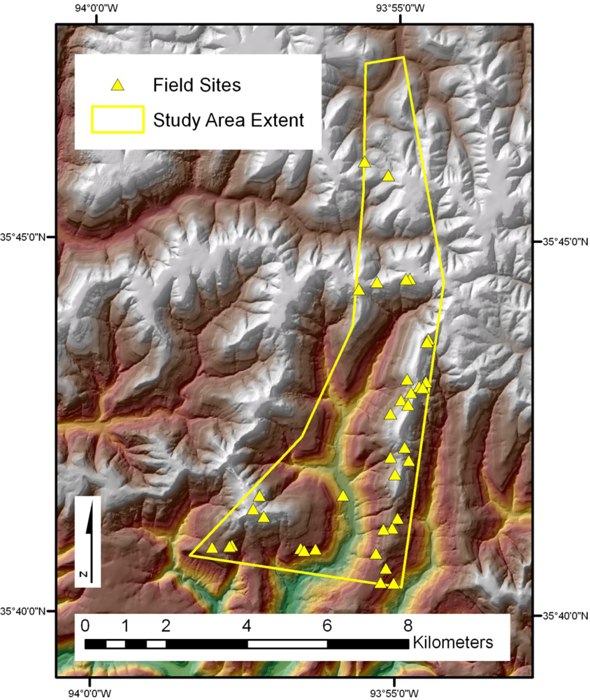
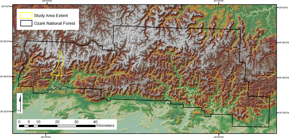
The 32 km2 study area (Figure 1) was located within the Ozark National Forest in Arkansas. The area is blanketed in an oak-hickory forest defined as an even mixture of upland oak and hickory [40]. The entire area of interest is contained within a box defined in latitude and longitude by an upper left-hand corner at 93°58′27″W and 35°47′24″N and a lower right-hand corner at 93°54′11″W and 35°40′22″N. The study area is contained within the Delaney and Bidville USGS [41] 7.5-min quadrangles. The relief of the study area ranges from 247 to 734 m above mean sea level. Spatially distributed in situ and remote sensor data were collected within the study area as described below.
2.2. Spatial Data
2.2.1. In Situ Reference Data
Within the study area, in situ sampling was conducted randomly within a stratum of interest, a practice widely used by foresters [15,42]. A GIS-based site suitability model, described in detail in Section 3.1, was developed to map the stratum and to select a random set of field sample plots according to topography, vegetation type, proximity to a road and land ownership. In situ measurements of tree diameters at breast height (DBH) were collected in October and November, 2008. A total of 27 plots were sampled (Figure 2) within the study area.
In situ sampling of basal area was the main field component of this study. Standard methods for the measurement of basal area [10,15] were used in the selected field sites. Basal area was calculated from a prism measurement of diameter at breast height (DBH) of all trees within the plot areas based on the following:
where BAF is the basal area factor measured in square feet per acre, W is the diameter of the circular cross section of the target and D is the distance from the vertex of the angle to the target. This same equation is used to calibrate the BAF of an angle gauge against a target with a circular cross section. The variables, W and D, must be measured in the same units. Mean basal area, g, was computed as: where G is plot basal area measured and N is the total number of measured trees in a plot. This is a more useful reference variable as it applies to the aged oak-hickory stands of the Ozark Plateau [19]. For this reason, the latter Equation (2) was incorporated in this study.First Bitterlich [43], and then Grosenbaugh [44,45], realized the application of sampling proportional to some characteristic of individuals in a population. This technique is referred to as probability proportional to size (PPS) and is widely used by foresters in basal area sampling. The most frequent application of PPS in forest sampling is horizontal point sampling. Under this schema, the probability of selecting a tree is proportional to the basal area of that tree. Horizontal point sampling usually occurs using a calibrated angle gauge, such as a prism [13]. This study used two calibrated optical prisms as angle gauges. The BAF is determined through the geometric relationship between the width of a target, the distance between the target and the angle of the gauge used [10].
2.2.2. Hyperion Hyperspectral Imagery
The Hyperion hyperspectral imagery is comprised of 220 spectral bands with wavelengths ranging from approximately 0.4–2.5 μm and nominal bandwidths of 10 nm. Hyperion was engineered with two separate linear arrays, including visible near-infrared (VNIR) and short-wave infrared (SWIR) spectroradiometers with a nominal spatial resolution of 30 × 30 m (USGS 2009). The Level 1 GST product acquired from USGS had incorporated a terrain correction using a digital elevation model (DEM) based on the February 2000 Shuttle Radar Topography Mission (SRTM) flown on Space Shuttle Endeavor. The spectral data were organized as an 8 × 40 km swath in a band-interleaved-by-line (BIL) format with a signed 16-bit data structure.
2.2.3. LIDAR-Derived Normalized Height Percentiles
The LIDAR-derived normalized height percentiles were generated using a 10 × 10 m moving neighborhood across a 1 × 1 m grid. Each point in the grid was processed using the neighborhood to calculate (1) a minimum elevation and (2–12) eleven normalized height percentile (NHP) surfaces [21]. These included the 5th, 15th, 25th, 45th, 55th, 65th, 75th, 85th, 95th and maximum (100th) percentile heights (in m) above the minimum. Riggins et al.[21] incorporated these same twelve LIDAR-derived vertical structure statistics in a regression tree biomass model using Cubist [46]. The machine learning feature selection process within Cubist revealed that the 15th and 100th percentile layers from the LIDAR data were the most useful descriptive statistics for predicting biomass (in kg/ha). As a comparative linkage, these same descriptive statistics were utilized in the present study for evaluating Hyperion information content with respect to vertical structure.
2.3. Data Processing Setup
The data utilized in this study comes from a range of sources; each data element had its own associated geographic information, spatial resolution, footprint size and format. All spatially-distributed variables were preprocessed to ensure uniform geographic projections. For the convenience of leaving the Hyperion hyperspectral imagery in its original projection, the WGS84 UTM Zone 15 N coordinate system was set as the standard geographic reference. All variables to be included in the project were formatted to allow their inclusion in an ASCII text file, and data were subset to the boundaries of the study area (Figure 1).
Remote sensor derivatives for model inputs and other derivatives, such as slope and aspect, were generated using the ESRI ArcGIS and ERDAS Imagine platforms.
2.4. GIS and Remote Sensing Constraints on Field Sites
To select sites for field sampling within the study area, a GIS model was designed to meet the needs of limited in situ data collection resources and the nature of the remote sensor derivatives. First, due to the nature of the LIDAR-derived statistics, reported previously by Riggins et al.[21], it was determined that analysis would need to be constrained to samples within a similar slope range, since the calculation of the LIDAR-derived neighborhood height statistics did not take slope into account. (The neighborhood elevation range on a steep slope is significantly higher than on flat topography with the same forest vegetation, and calibration of the data to incorporate the slope was beyond the scope of this study.) Second, a simple random sample of field sites within the study area would produce many useless sites (e.g., open fields or other areas not dominated by oak or hickory); therefore a stratified random sample was selected. Third, the positions and 30 × 30 m horizontal dimensions of the Hyperion pixels constrained how point sites were addressed in situ. Sample sites covered an area of a pixel with geolocational errors compensated for in the sampling methodology.
3. Methods
3.1. Site Selection Model
The input layers for the GIS-based field plot site selection model included (1) minimum LIDAR point elevation within each 10 × 10 m neighborhood, (2) each of the eleven normalized height percentile (NHP) surfaces representing vegetation canopy, (3) percent forest canopy cover, (4) high potential for evergreen, (5) Forest Service roads, (6), ridge top polygons and (7) the study area boundaries. The spatial resolution of the first two input layers (1,2) was 1 × 1 m and the resolution of the remaining raster layers (3,4) was 30 × 30 m. Differences in raster spatial resolution and in coordinate systems necessitated the standardization of projections and spatial resolutions between all data elements.
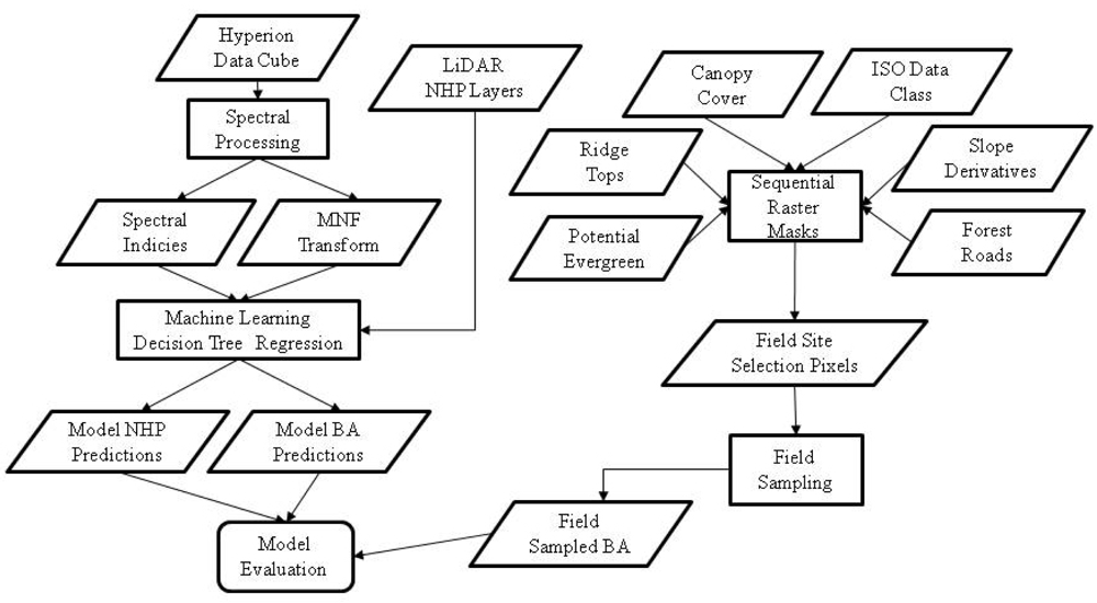
From the first NHP layer, both slope and aspect were generated and clipped to the extent of the study area. The base elevation from the LIDAR derivatives and the canopy layers were individually clipped and subsequently compiled into a multiband raster file prior to ISODATA clustering. The final number of classes was decided on through iterative visual inspection; a maximum of 20 classes was selected as the desired output, though 17 classes were actually generated. The ISODATA classes were then used to differentiate forest cover containing oak-hickory from other forest cover types. Once the various input layers were compiled, they were combined as successive masks (Figure 3).
A primary goal in the site selection model was to restrict the slope to a range from 0 to 15 degrees, with the assumption that this is sufficient to remove or minimize the influence of NHP canopy data not calibrated for slope within the LIDAR point cloud. A secondary goal of the site selection process was to ensure that input pixels contained only oak-hickory forest cover. The resulting raster was converted to a polygon layer and a random sample of points was generated within its confines. All of these points were separated by at least 30 m (the dimension of a Hyperion pixel).
Of the 17 ISODATA clusters generated, seven contained a majority of oak-hickory forest cover. These seven classes were combined with only slope in the 0–15 degree range, and the output was combined with the canopy cover layer as an additional mask to remove pixels containing a majority of open fields and roads. The selection criteria included only canopy classes with 85%–95% cover. A subsequent visual comparison of the ISODATA classes to a high resolution DOQQ image identified pine stands that were included in the seven classes above. In order to fully separate all oak-hickory and evergreens into unique classes, a potential evergreen layer was added to remove pine trees that had been misclassified into oak-hickory classes. Slope aspect was used to further reduce the potential sampling zone area. The aspect was limited to south, southwest, north and northeast aspects identified as being of particular interest to oak-hickory decline research at the University of Arkansas Forest Entomology Lab.
Ridgetop polygons developed by Tullis et al.[47] were buffered by 250 m and subsequently used as a raster mask. The ridgetops ensured sites were well drained (not riparian zones) with similar topography and also corresponded with the team’s interest in red oak borer-induced stresses in Ozark National Forest. Finally, an additional buffer zone of 250 m from forest roads was used to maximize site accessibility with the resources that were available. The output from this final step was converted from a raster format to a vector-based polygon layer. Within this polygon, a random set of points (separated from each other by at least 30 m) was generated.
3.2. Field Sampling Methods
Plots were sampled in the Ozark National Forest based on a random sample of 27 points generated by the site selection model. A horizontal point sampling scheme was used based on the probability proportional to size (PPS) method [13]. The actual in situ sampling method employed a pair of calibrated prisms as angle gauges.
Plots were located using a GPS receiver (Trimble Juno) with an external antenna attached to the hat of the surveyor. Upon reaching the point indicated by the receiver, trees were sampled from the center of the plot using the BAF 10 prism supplemented by the BAF 1 prism every third plot. Two prisms were used to ensure accurate sampling across variations in the forest cover within the study area.
Each prism was held at eye level over the designated center of the plot. The observer rotated around the prism in a full 360 degree circle sighting on each tree in view. Trees were identified as being included in the sample using the prism optical angle gauge. At least four in situ photographs were taken at right angles to one another from the center of each plot, allowing a visual reference of site conditions. Care was taken in the conversion of English units to metric units for the calculation of basal area. Conversion was necessary because the units of measurement on the BAF 10 prism were ft2 per acre, while the units on the BAF 1 prism were m2 per hectare.
3.3. Spectral Processing
The NASA EO-1 Hyperion imagery was provided in radiance values recorded in a signed 16-bit data structure in the GEOTIFF file format. The radiance values were supplied in scaled digital numbers (DN) with units of W·m−2·sr−1·μm−1. For the bands from the SWIR sensor, the radiance values were scaled by a factor of 80, and the VNIR bands were scaled by a factor of 40.
Using a simple band math function, the supplied radiance values were converted to reflectance using the following equation:
where ρP is the unitless planetary reflectance, Lλ is the spectral radiance at the sensor for wavelength λ, d is the distance between the Earth and the Sun in astronomical units (AU), ESUNλ is the Hyperion solar radiance in W·m−2·sr−1[41] for wavelength λ and θs is the solar zenith angle in degrees [48].A visual inspection was performed on the Hyperion signal-to-noise ratio (SN) stack and bands containing high levels of noise were identified. Bands identified in accompanying Hyperion metadata as non-calibrated were also removed, resulting in a final image stack containing 135 bands from the original 220 band Hyperion image. Noise was evaluated over the confluence of the Mulberry and Arkansas rivers captured in the southern third of the Hyperion hyperspectral image. These two water bodies provided regions of uniform spectra against, whose noise could be visually evaluated. The bands used in the spectral derivatives discussed in the next section were taken from the 135 band image stack. This represents a 56% reduction from the raw Hyperion image stack. The resulting bands were spatially subset to match the extent of the study area.
3.4. Hyperspectral Indices
Modified normalized difference (mND) and modified simple ratio (mSR) are two indices that have been found to function better with hyperspectral imagery than the standard normalized difference or the simple ratio [49]. In the model utilized in this study, the mND and mSR were calculated using Equations (4) and (5). In this case, ρ1 is 1,194.97 nm (band 105), ρ2 is 2,224.03 nm (band 207) and ρ3 is 915.23 nm (band 56) from the Hyperion hyperspectral image stack.
Normalized difference vegetation indices (e.g., NDVI) have been used for many years by researchers to track vegetation changes [17,50]. There have been many modifications of the basic NDVI and for this project the narrow band NDVI described by Thenkabail et al.[51] was used. Equation (6) is taken from Thenkabail et al.[51], but for this research, it was modified by using 813.48 nm (band 46) and 609.97 nm (band 26) in place of ρ860 and ρ660, respectively. This change was made to avoid noise bands while maintaining the spectral separation between reflectance values.
The canopy structure index (CSI) was developed by Sims and Gamon [50] as a tool for extracting the variability in canopy density across the landscape. They use scaled versions of the simple ratio (SR) and water index (WI). The inclusion of these two scaled indices was calculated to allow a wider applicability of the CSI. They found that he SR works best on thin canopies, while the WI works best on thicker canopies. Including a scaled version of both these two indices allows the CSI to function in a differential way as the canopy varies. Equations (7)–(9) are taken from Sims and Gamon [50], and in this instance (WI1180 – 1)max ≈ 206.2255 and (SR680 – 1)max ≈ 11.4154. The reflectance values used in calculating the CSI for ρ680, ρ800, ρ900 and ρ1180 are 681.20 nm (band 33), 803.30 nm (band 45), 905.05 nm (band 55) and 1,184.87 nm (band 104) from the Hyperion image stack, respectively.
A normalized difference water index (NDWI) is used by researchers to obtain information on vegetation canopy water content [50,52–54] and typically does a better job at detecting plant stress and biomass changes than other more traditional vegetation indices [55]. NDWI was calculated for this study using Equation (10) where ρ1235 is 1,235.27 nm (band 109) and ρ854 is 854.18 nm (band 50) of the Hyperion image.
The red edge position (REP) has been used successfully in previous studies [16,56,57] to extract forest biophysical variables from hyperspectral data. The REP layer used in this study was generated with Equations (11) and (12), where ρ742 is 742.25 nm (band 39), ρ701 is 701.55 nm (band 35), ρ671 is 671.02 nm (band 32) and ρ782 is 782.95 nm (band 43) of the Hyperion image [16,56].
Double Difference index (DDn) is based on a difference between derivatives of the reflectance. The DDn is calculated using the difference of the integral of reflectance derivatives, where a and b are different wavelengths and Δ is the integration window. This index has been found to be useful at the canopy level for detection of biophysical variables. It has the advantage of being computationally simple, yet maintaining the hyperspectral characteristics of the data. The simplified DDn used here is provided in Equation (13) [58]. The input reflectance bands used were as follows: Ra is 721.90 nm (band 37), Ra+Δ is 752.43 (band 40), Rb is 671.02 nm (band 32) and Ra+Δ is 701.55 nm (band 35). In this case, a value of 30 nm was used for Δ.
3.5. Minimum Noise Fraction Transformation
The MNF works through a linear process consisting of two separate principle components analyses. A MNF transformation requires a normal distribution in the data; typically most software applications perform a normalization procedure on the data prior to the MNF transformation. The first PCA uses the noise covariance matrix to decorrelate and rescale the data generating a transformed data set with unit noise variance and no between-band correlations. The second PCA uses those values derived by the first PCA to output PCA-like bands ordered relative to the signal-to-noise values [59]. The MNF determines the inherent dimensionality of the data and it is also useful to segregate the noise from the signal in the data.
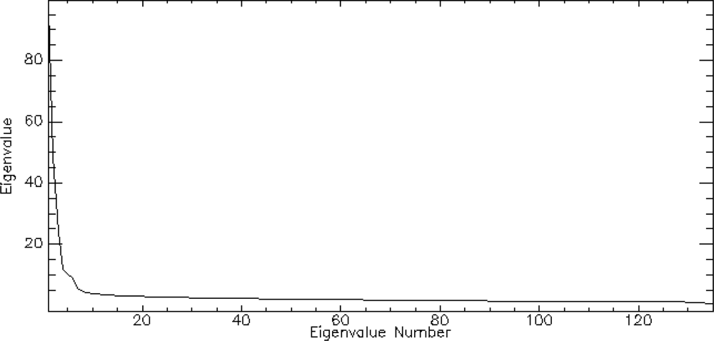
A minimum noise fraction transformation was performed on the 135 bands of the noise reduced and spatially subset Hyperion image stack. An existing commercial algorithm contained within the ENVI MNF process was used to estimate noise statistics from the data, since there were no statistics derived from in situ collection for the imagery in question. The first six components of the forward MNF transformation were determined to contain signal information; the stack of 135 bands of Hyperion hyperspectral image was reduced to six MNF components.
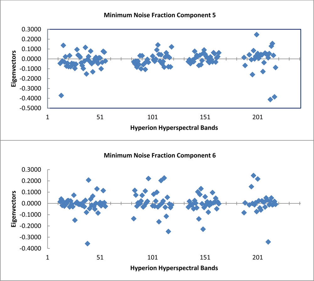
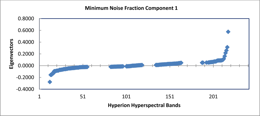
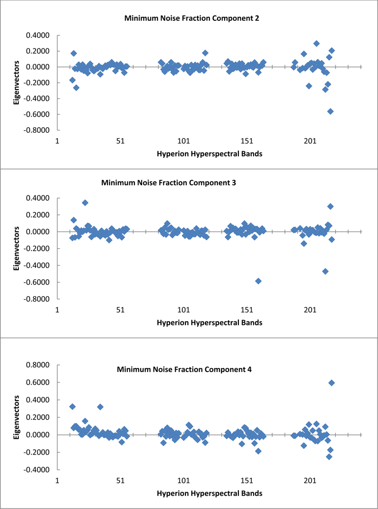
The graph of the eigenvalues shows a clear break point at 9.0 (Figure 4). The eigenvectors resulting from the second principle components rotation preformed as part of the minimum noise fraction transformation show, which spectral bands were important in the generation of each MNF component band (Figure 5). The spectral regions that seem to contribute the most to the first six MNF components are all in the infrared region of the electromagnetic spectrum (Table 1).
3.6. LIDAR Normalized Height Percentile Layers
From the LIDAR data, normalized height percentile layers (15th, 25th, 45th, 55th, 65th and the maximum) were resampled from 1 × 1 m spatial resolution to 30 × 30 m using a block statistics process. This function resampled the raster data using non-overlapping neighborhoods. The 30 × 30 m pixels that were generated were assigned the mean value of the 1 × 1 m pixels within each 30 × 30 m neighborhood. These data layers were used in the machine learning process as dependent variables.
Regression tree rule sets were generated using the Cubist 2.06 machine learning decision tree [46]. An iterative “brute force” implementation of Cubist was used as a first step to search for patterns in the preprocessed Hyperion data. A configuration file was generated for every possible combination of a single dependent variable and up to nine independent variables derived from the Hyperion hyperspectral data. No more than nine independent variables were included in any “brute force” implementation due to time constraints of a single computer workstation. (For each set of models that were run, 511 variations were generated for each dependent variable, resulting in a total of 3,066 output rule sets.) At least one independent variable was included in each of the resulting rule sets.
3.7. Machine Learning Decision Tree Regression
In the discussion of the machine learning methods and results, it is important to ensure clear terminology. In the work presented here, the word “rule set” will be used to refer to a single output rule set from the machine learning regression tree procedure. Each set of models will be referred to as an “epoch.” Each epoch is conducted using a different subset of independent variables. The performance of a particular rule set is evaluated on the basis of the average error, relative error, correlation coefficient and RMSE associated with that rule set. The average error is the absolute value of the difference between the predicted rule set and the actual rule set averaged over all of the instances of the input. The relative error is also generated by Cubist and is used to indicate the usefulness of the model. The relative error reported by the software must be less than 1 to indicate a useful rule set. The correlation coefficient is a measurement of the agreement between the actual values of the predicted variable and the rule set generated values for that variable.
The normalized height percentiles used in the model were determined based on the work of Riggins et al.[21]. Predicting the results of a previous model prediction might result in a compounding of the associated error, thus the machine learning was applied to find a model to predict the actual LIDAR inputs used by Riggins et al.[21] in their biomass model, which allowed for a more direct assessment of vertical forest structure via the Hyperion hyperspectral data.
3.8. Hyperion to NHP and Basal Area Predictions
The first stage of the forest structure assessment process was a search of the Hyperion hyperspectral image derivatives in order to determine the nine independent variables that yielded the most accurate predictions of each NHP layer. The data set used in this phase of the research included 7,284 (30 × 30 m) pixels.
Regression was performed using a set of six dependent variables (the six NHP layers) taken from Riggins at al.[21]. There were 14 independent variables included. These were the mND, mSR, NDVI_nb, CSI, NDWI, REP, DDn, aspect and the first six bands of a forward minimum noise fraction transformation all derived from the Hyperion hyperspectral data.
Of the 14 independent variables, a subset of nine variables was selected for each epoch. The number of inputs was limited to ensure speedy processing and a manageable number of outputs for each epoch. With the six dependent variables (NHP layers) and the nine independent variables, the total number of parameters input into the data mining application was 15 per epoch. The number of combinations was 511 after removing the case of no independent variables included, making a total of 3,066 rule sets per epoch. With Cubist, the associated outputs from the modeling (four files per epoch) and the output results, the number increased seven-fold to 21,462 files generated per epoch, thus approaching the limits of efficient file management capabilities on a typical workstation.
An iterative approach was used to determine the best subsets of independent variables for predicting each of the dependent variables. The top performing rule set for each dependent variable was located in the output file and the variables included were noted. For each epoch, the total number of times an independent variable was used across all six dependent variables determined if it was carried into the second epoch. This approach was used until all fourteen independent variables had been included in at least one epoch. Next, the same evaluation criteria were used to select the nine top performing independent variables from the two epochs. These nine top performing variables were then input into a third and final epoch.
The second stage of the modeling process was intended to provide validation of the independent variable selection from the data mining process. A series of rule sets were developed on a 15% random sample of pixels from the 7,284 available pixels, resulting in a sample of 1,087 pixels. These models were then tested against a non-overlapping secondary sample of 1,087 pixels.
A further structure detection step was performed to attempt to predict a known biophysical variable. The field basal area measurements were substituted into the rule sets generation process as the sole dependent variable. Based on the results from the data mining stage, a single epoch was performed to predict basal area. The rule set inputs were taken from the top performing subset in the NHP predictions. These results were evaluated on the basis of the average errors associated with each output.
A single training epoch was performed on all 27 field sampled points. This provided a point of comparison for the validation results. Because the field-intensive sample contained only 27 data points, a set of 50% training/test sample partitions was unrealistic. A 10-fold cross validation epoch was used as the validation of the training on the basal area prediction rule sets. The 10-fold cross-validation epoch took the full data set and blocked it into 10 blocks of roughly the same size. Each block then had a rule set constructed from the elements in the remaining nine blocks, and this rule set was tested against the hold-out block elements. The overall rule set results were estimated by averaging all the hold-out case results.
4. Results
4.1. In Situ Field Samples
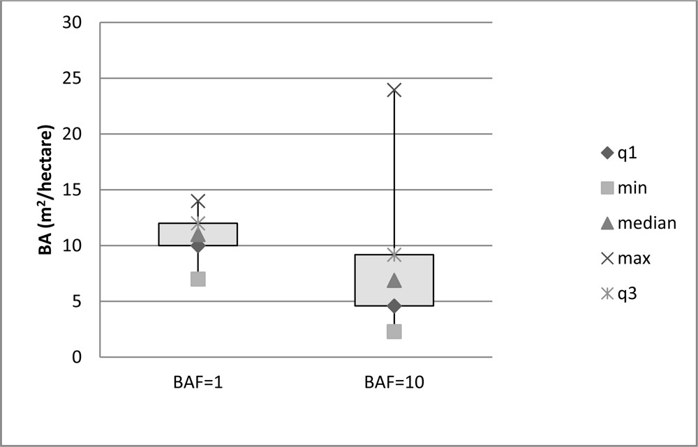
The in situ field sampling produced basal area estimations for 27 field plots. The prism angle gauge used sampled plots at a variable radius, which was determined by the DBH of the trees in the area. On average, the plots covered an area at their extreme radius of ∼80% of a 30 × 30 m pixel. The spatial separation between plots (Figure 2) ensured that no overlap occurred between any two sampled pixels. The in situ field data collected was compiled and basal area calculated from the BAF of the prisms used. Photographs at each of the field plot sites enhanced understanding of the spectral results (Figure 6).
Variability of the basal area apparent in the sampling across the study area was within the expected range. The distribution of the basal area sampled (Figure 7) was different between the two prisms (BAFs). The BAF 10 prism shows a larger spread in the distribution with a distinct skew, while the BAF 1 shows a narrower spread with a normal distribution.
4.2. Hyperion to Predict Normalized Height Percentiles
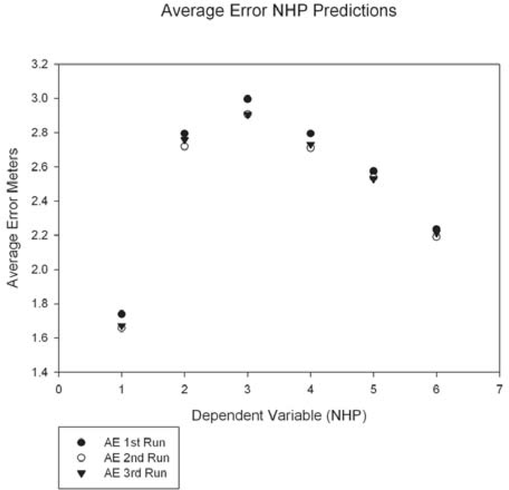
The rule sets generated by each NHP training epoch were evaluated and the top performing models from each epoch, along with the independent variables included in that model, were examined and evaluated. The average error values for each of the three epochs ranged from (1) 1.73–2.99 m, (2) 1.65–2.90 m and (3) 1.67–2.90 m. The ranges on the correlation coefficients were 0.42–0.47, 0.45–0.51 and 0.45–0.50 for epochs one through three, respectively. The RMSE accuracy ranged between 2.18–3.78 m for the first epoch, 2.08–3.69 m for the second epoch and 2.10–3.7 m for the third epoch (Table 2). For the purpose of this study, it was determined that a correlation coefficient of 0.50 would represent a medium positive correlation.
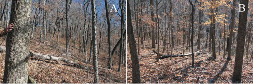
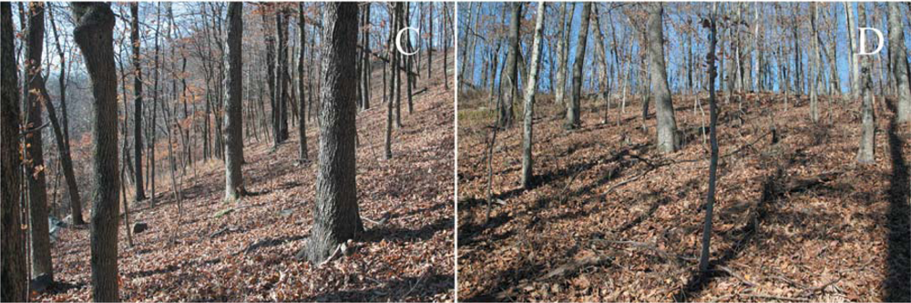
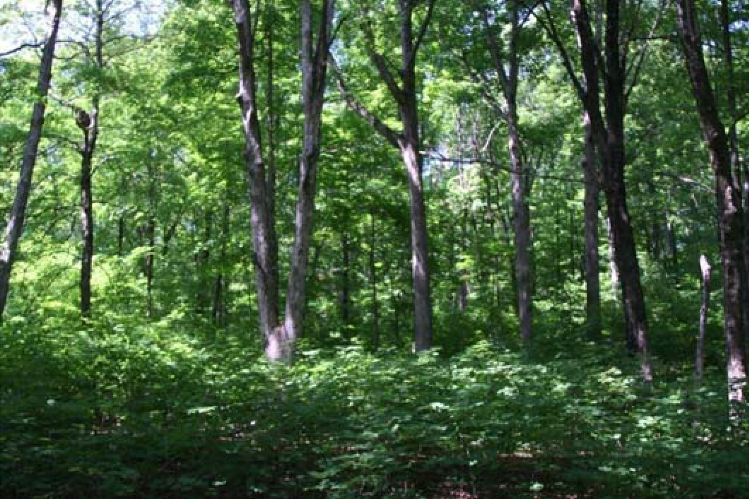
Minor decreases in the average error and RMSE were inversely mirrored by increases in the correlation coefficients of the results with the iterative approach used. The consistent pattern that emerged showed a higher accuracy in predictions on NHP 15% and NHP maximum relative to the other four NHP layers (Table 2). Typical structure in the oak-hickory forest consists of a lower understory followed by several meters of limbless trunk with spreading canopy at the very top (Figure 8). Since the highest accuracy is in predicting the lowest and highest NHP layers, it is likely that the spectral data contain structural information related to the understory and the canopy tops. Inherently, the spectral data represent the canopy most visible from space so the higher accuracy in predicting the NHP maximum makes sense from both a remote sensing and a field survey perspective.
The graph of the average errors for the three runs (Figure 9) shows an arc plot pattern with dependent variable 1 (NHP 15%) and dependent variable 6 (NHP maximum) at the lower ends and dependent variables 2–5 (mid-regions of the canopy from the NHP layers) in the peak region. Since we utilized models to predict height from spectral data, we would expect the NHP maximum to be the most accurate prediction, as it represents the top of the forest canopy. The higher accuracy in predicting NHP 15% is harder to explain. One possibility is that this represents the influence of the understory on the spectra. The lower understory canopy may show the influences of additive reflectance [17] allowing it to be used to predict the NHP 15% layer by the spectral data. As has been pointed out by previous researchers [60–62], the understory reflectance can be a major influence on spectral remote sensing of forest biophysical variables.
Of the three epochs, the first two were to ensure inclusion of all 14 independent variables at least once in an epoch. The set of 14 independent variables was subset to nine inputs to allow efficient processing and to conserve disk space. The independent variables included in the third epoch were selected from the top performing models of the first and second epochs. For CSI, aspect, MNF1 and MNF4 variables, each appeared in all six rule sets from both the first and second epoch. For NDVI, NDWI, REP, DDn and MNF3 variables, each appeared in five of the six rule sets from the first or second epoch. These nine variables were considered the top performing independent variables and were included in the third and final epoch (Table 2).Plots of average error by each dependent variable (or NHP layer) from the top performing models also show similar patterns (Figure 9). These results are as expected as the canopy is the most important part of the spectral data. Upon evaluation of the results from the three data mining epochs it was apparent that the outputs changed only slightly as the inputs were refined. The second epoch consisting of independent variables CSI, DDn, aspect and MNF band 1–6 was producing rule sets with the lowest average error and the highest correlation coefficients. Accordingly, these input variables were selected for use in the validation phase of the modeling.
Typically, the second epoch results were more accurate for the NHP 15% and NHP maximum predictions. The results showed some variation in the middle four dependent variables, suggesting that each dependent variable may be more accurately predicted by specific independent variables. It was thought at first that it might be an over simplification to try and predict all six dependent variables using the same set of independent variables. Upon closer examination of the results, however, it is apparent that the nine independent variables selected for each epoch do not show a bias toward the middle NHP layers, so further iterations are not likely to produce new results even if tailored specifically to a specific dependent variable.
4.3. Hyperion to NHP Prediction Validation Phase
Based on the machine learning steps described in the previous section, a subset of independent variables, CSI, DDn, aspect and MNF band 1–6, was determined to produce the most accurate rule sets for NHP prediction from the hyperspectral data derivatives. A set of rule sets were run on the data set using a 15% random sample of points as a training set, containing 1,087 data points. Once these rule sets were generated, they were evaluated against a second non-overlapping random sample consisting of a further 1,087 points.
On the 15% training section (Table 3), the top model results predicted canopy heights ranging from 1.97 to 3.17 m in the average error column with accuracies between 2.16–3.75 m based on the RMSE. The correlation coefficients for the test ranged from 0.25 to 0.34. The 15% test reported average errors between 1.78 and 3.07 m with accuracies between 2.20 and 3.91 m based on RMSE and correlation coefficients ranged from 0.34 to 0.41. Based on these results, Hyperion hyperspectral data may have utility for predicting structural information contained in a small footprint LIDAR-derived surface.
4.4. Hyperion to Basal Area Prediction
Unlike prediction of LIDAR-derived statistics, results indicated that we are not able to accurately predict basal area within our study. Based on the 27 pixels supported by field sampling of basal area included in a Cubist training dataset, the RMSE for the training phase of the basal area model was high at 4.97 m2/ha. Some models failed to produce any useful results, and some of the models showed a flat-line or a tendency for results to be plotted at a single prediction value (constant) with the results stretched the entire length of the reference axis. In these results, the best average error ranged from 6.55 m2/ha to 6.72 m2/ha. The correlation coefficients for the basal area prediction were less than 0.30 (Table 4).
5. Discussion
The combination of hyperspectral imagery with LIDAR-derived height statistics to evaluate structural information contained in the spectral data provides an exciting field of possibilities for remote sensing of forested environments. Of particular note is the ability to roughly estimate canopy height of the understory in the study area (RMSE = 2.2 m). In contrast, the inclusion of in situ data in the evaluation of the basal area prediction allowed field-based evaluation of the prediction results. The fact that these data were collected based on a set of parameters determined primarily by the LIDAR data is highly important. Given that, in this study, sites were sampled within a narrow range of slope values, a more thorough evaluation of the data will require LIDAR-derived statistics calibrated for surface topography. In situ sampling used for a biophysical variable might be expanded to include multiple slope ranges and comparisons between these ranges made to determine the influence of slope on any structural information that can may be extracted from the hyperspectral data.
The top performing models were able to predict NHP to within 1.6 m or 2.2 m, for NHP 15% data and NHP maximum data, respectively (Figure 9). Considering the data used was collected using a single space-based sensor and given the accuracies reported here for predictions of forest canopy height, there is the potential for future applications of combined hyperspectral and LIDAR data in remote sensing of forest structure. The influence of additive reflectance from energy transmitted through the upper canopy [17] may be one reason behind the higher accuracy in predicting the lowest NHP layer over the maximum NHP layer. However, the canopy scene is complex and the ability to sort out exactly why different structures alter the spectra could be difficult to ascertain. From the standpoint of machine learning decision tree regression, the naturally smaller vertical range of NHP 15% should also be considered as a possible factor when interpreting its relatively higher accuracy. Based on our work, rough estimates of basal area from orbital hyperspectra may be more difficult. Of course, a relatively small number of in situ sites could be dramatically increased (with significant time and expense) in an attempt to improve rule set development.
Numerous attempts have been made to measure forest biophysical characteristics using multispectral data, hyperspectral data and various combinations of the two. Hall et al.[49] used Landsat TM to map coniferous understory in a Canadian forest. Xain [63] also attempted an assessment of forest structure using forest inventory data and Landsat ETM+ imagery; however, their best results had an associated error of 51%–75%, which does not meet the accuracy requirements of 80% established for forest inventory by the USGS National Park Service Vegetation Mapping Program [64]. Hyde et al.[31] combined hyperspectral data with LIDAR data to successfully increase the accuracy of spectrally derived biophysical variable measurements. Kalacska et al.[65] use spectral remote sensing with EO-1 Hyperion hyperspectral satellite imagery to estimate forest structure in dry tropical forests. Chopping et al.[66] measure canopy characteristics using NASA multi-angle imaging spectro-radiometer (MISR) data. They worked in a shrub and coniferous dominated region of southeastern Arizona and southern New Mexico, measuring woody biomass, canopy cover and mean canopy height. They conclude that multi-angle spectral data has uses in detecting biophysical variables. Palace et al.[67] used panchromatic IKONOS imagery to analyze tree crowns in a Brazilian forest, accurately determining field measured crown widths. Schlerf and Atzberger [68] model canopy structure variables in Norway spruce stands using airborne HyMap data building a link between HyMap hyperspectral and Landsat through a model called INFORM.
Hyperspectral remote sensing has been successfully used by researchers to identify individual species within the forest. Ramsey et al.[69] use Hyperion hyperspectral data to identify and map the location of Chinese Tallow (Triadica sebifera) encroachments in the southern and southeastern regions of the United States. Cochrane [70] used a hyperspectral sensor in conjunction with a simple algorithm to discriminate species in a Brazilian tropical forest. The ability to use hyperspectral data to identify species, illustrated by researchers like Ramsey et al.[69] and Cochrane [70], in addition to the structural information derived in this study suggest hyperspectral remote sensing has the potential to be a powerful tool in forest evaluation and monitoring. Additional questions that might be addressed or clarified through future research are: (1) Does space-based (e.g., Hyperion) hyperspectral data contain sufficient structural information to predict forest biophysical variables in forest conditions beyond the oak-hickory data examined here? (2) What advantages are gained through the use of a single hyperspectral image vs. multispectral data acquired on multiple dates? (3) Can the intensity of field sampling and/or its spatial aggregation enhance the prediction of biophysical variables related to structure when compared with synergies between LIDAR and hyperspectral remote sensing?
6. Conclusion
From the results of this study, it is clear the Hyperion hyperspectral image data contains patterns related to vertical forest structural information. The data mining approach used in this study isolated a set of hyperspectral derivatives that were used to predict canopy structure in the oak-hickory forest of Ozark National Forest. These derivatives were used in a series of regression model predictions, which confirmed that the Hyperion hyperspectral data contains extractable structural information related to forest canopy height. The predictions of the LIDAR-derived understory and maximum canopy heights were the most promising, with accuracies ranging from 2.2 to 3.91 m RMSE. In contrast, efforts to extract basal area information content were not as promising (6.5 m2/ha RMSE when the average basal area across the study area was ∼12 m2/ha). The study demonstrated specific applicability of hyperspectral remote sensing (by itself) in assessment in the oak-hickory dominated forests of the Ozark National Forest. This procedure can be used as a preliminary comparison for related methods of forest evaluation, monitoring or inventory by providing information that allows the focused application of more intensive machine learning and/or expensive in situ methods in the areas of greatest need.
The nature of this structural information is related to characteristics of the canopy, which is indicated by the higher accuracies of predictions for the lowest (understory) and the maximum (top of the canopy). A spectral remote sensor-based rapid estimation technique for rough forest structure has potential for forestry, biology and ecology applications. Such a measurement technique will allow the tracking of forest conditions due to natural and anthropogenic influences over large tracts of forest. Additionally, continued improvements in forest structural assessment will allow more efficient and frequent evaluations of forest condition and biophysical parameters, as well as a basis for continuous monitoring of forest condition through time.
The authors gratefully acknowledge support provided by the University of Arkansas Agricultural Experiment Station, the Department of Entomology and the Center for Advanced Spatial Technologies; the project was funded by grants from the USDA Forest Service Southern Research Station and by AmericaView.
References
- Battles, J.J.; Fahey, T.J. Gap dynamics following forest decline: A case study of red spruce forests. Ecol. Appl 2000, 10, 760–774. [Google Scholar]
- Binkley, C.S. Climatic change and forests. Science 1989, 243, 991. [Google Scholar]
- Scott, J.T.; Siccama, T.G.; Johnson, A.H.; Breisch, A.R. Decline of red spruce in the Adirondacks, New York. Bull. Torrey Bot. Club 1984, 111, 438–444. [Google Scholar]
- Chen, J.M.; Black, T.A. Defining leaf area index for non-flat leaves. Plant Cell Environ 1992, 15, 421–429. [Google Scholar]
- Blodgett, C.F.; Jakubauskas, M.E.; Price, K.P.; Martinko, E.A. Remote Sensing-Based Geostatistical Modeling of Forest Canopy Structure. Proceedings of ASPRS 2000 Annual Conference, Washington, DC, USA, 22–26 May 2000.
- Manion, P.D. Evolution of concepts in forest pathology. Phytopathology 2003, 93, 1052–1055. [Google Scholar]
- Wardle, D.A.; Walker, L.R.; Bardgett, R.D. Ecosystem properties and forest decline in contrasting long-term chronosequences. Science 2004, 305, 509–513. [Google Scholar]
- Kasischke, E.S.; Goetz, S.; Hansen, M.C.; Ustin, S.; Ozdogan, M.; Woodcock, C.E.; Rogan, J. Temperate and Boreal Forests, 3rd ed.Ustin, S.L., Ed.; John Wiley & Sons: Hoboken, NJ, USA, 2004; Volume 4, p. 736. [Google Scholar]
- Rubin, B.D.; Manion, P.D.; Faber-Langendoen, D. Diameter distributions and structural sustainability in forests. Forest Ecol. Manage 2006, 222, 427–238. [Google Scholar]
- Wenger, K.F. Society of American Forestry Handbook; Wiley: New York, NY, USA, 1984; p. 1335. [Google Scholar]
- Skelly, J.M. A. Closer Look at Forest Decline: A Need for More Accurate Diagnostics. In Forest Decline Concepts; Manion, P.D., Lachance, D., Eds.; APS Press: Saint Paul, MN, USA, 1992; pp. 85–107. [Google Scholar]
- Franklin, S.E. Remote Sensing for Sustainable Forest Management; Lewis Publishers: Boca Raton, FL, USA, 2001; p. 407. [Google Scholar]
- Husch, B.; Beers, T.W.; Kershaw, J.A.J. Forest Mensuration, 4th ed.; John Wiley & Sons: New York, NY, USA, 2003; p. 443. [Google Scholar]
- Schreuder, H.J.; Gregoire, T.G.; Wood, G.B. Sampling Methods for Multiresource Forest Inventory; John Wilet & Sons: New York, NY, USA, 1993; p. 446. [Google Scholar]
- West, P.W. Tree and Forest Measurment; Springer: Berlin, Germany, 2004; p. 167. [Google Scholar]
- Jensen, J.R. Introductory Digital Image Processing: A Remote Sensing Perspective, 3rd ed.; Pearson Education INC.: Upper Saddle River, NJ, USA, 2005; p. 526. [Google Scholar]
- Jensen, J.R. Remote Sensing of the Environment: An Earth Resource Perspective, 2nd ed.; Pearson Prentice Hill: Upper Saddle River, NJ, USA, 2007; p. 592. [Google Scholar]
- Asner, G.P.; Hicke, J.A.; Lobell, D.B. Per-Pixel Analysis of Forest Structure: Vegetation Indices, Spectral Mixture Analysis and Canopy Reflectance Modeling. In Remote Sensing of Forest Environments: Concepts and Case Studies; Wulder, M.A., Franklin, S.E., Eds.; Kluwer Academic Publishers: Boston, MA, USA, 2003; pp. 209–254. [Google Scholar]
- Anderson, J.E.; Plourde, L.C.; Martin, M.E.; Braswell, B.H.; Smith, M.L.; Dubayah, R.O.; Hofton, M.A.; Blair, J.B. Integrating waveform lidar with hyperspectral imagery for inventory of a northern temperate forest. Remote Sens. Environ 2008, 112, 1856–1870. [Google Scholar]
- Hudak, A.T.; Lefsky, M.A.; Cohen, W.B.; Berterretche, M. Integration of lidar and Landsat ETM+ data for estimating and mapping forest canopy height. Remote Sens. Environ 2002, 82, 397–416. [Google Scholar]
- Riggins, J.J.; Tullis, J.A.; Stephen, F.M. Per-segment aboveground forest biomass estimation using LIDAR-derived height percentile statistics. GIScience Remote Sens 2009, 46, 232–248. [Google Scholar]
- Stone, J.N.; Porter, J.L. What is forest structure and how to measure it? Northwest Sci 1998, 72, 25–26. [Google Scholar]
- Leutner, B.F.; Reineking, B.; Bachmann, M.; Beierkuhnlein, C.; Dech, S.; Wegmann, M. Modelling forest a-diversity and floristic composition—On the added value of LiDAR plus hyperspectral remote sensing. Remote Sens 2012, 4, 2818–2845. [Google Scholar]
- Wynne, R.H. Lidar remote sensing of forest resources at the scale of management. Photogramm. Eng. Remote Sensing 2006, 72, 1311–1313. [Google Scholar]
- Mundt, J.T.; Streutker, D.R.; Glenn, N.F. Mapping sagebrush distribution using fusion of hyperspectral and lidar classification. Photogramm. Eng. Remote Sensing 2006, 72, 47–54. [Google Scholar]
- Foody, G.M.; Muslim, A.M.; Atkinson, P.M. Super-resolution mapping of the waterline from remotely sensed data. Int. J. Remote Sens 2005, 26, 5381–5392. [Google Scholar]
- Puzzolo, V.; Maselli, F.; Marchetti, M.; Buongiorno, F. Multi-Seasonal Classification of LANDSAT TM Images for Increasing Forest Type Discrimination in Mediterranean Environment. In Analysis of Multi-Temporal Remote Sensing Images; Smits, P., Bruzzone, L., Eds.; World Scientific: Hackensack, NJ, USA, 2003; pp. 322–329. [Google Scholar]
- Thornton, M.W.; Atkinson, P.M.; Holland, D.A. Sub-pixel mapping of rural land cover objects from fine spatial resolution satellite sensor imagery using super-resolution swapping. Int. J. Remote Sens 2006, 27, 473–491. [Google Scholar]
- Aplin, P. On scales and dynamics in observing the environment. Int. J. Remote Sens 2006, 27, 2123–2140. [Google Scholar]
- Townsend, P.A.; Foster, J.R.; Chastain, R.A.J.; Currie, W.S. Application of imaging spectroscopy to mapping canopy nitrogen in the forests of the central appalachian mountains using Hyperion and AVIRIS. IEEE Trans. Geosci. Remote Sens 2003, 41, 1347–1354. [Google Scholar]
- Hyde, P.; Dubayah, R.; Walker, W.; Blair, J.B.; Hofton, M.; Hunsaker, C. Mapping forest structure for wildlife habitat analysis using multi-sensor (LiDAR, SAR/InSAR, ETM+, Quickbird) synergy. Remote Sens. Environ 2006, 102, 63–73. [Google Scholar]
- Gemmell, F.M. Effects of forest cover, terrain and scale on timber volume estimation with Thematic Mapper data in a rocky mountain site. Remote Sens. Environ 1995, 51, 291–305. [Google Scholar]
- Peterson, D.L.; Westman, W.E.; Stephenson, N.J.; Ambrosia, V.G.; Brass, J.A.; Spanner, M.A. Analysis of forest structure using Thematic Mapper simulator data. IEEE Trans. Geosci. Remote Sens. 1986, GE-24, 113–120. [Google Scholar]
- Tokola, T.; Sarkeala, J.; van der Linden, M. Use of topographic correction in Landsat Tm-based forest interpretation in Nepal. Int. J. Remote Sens 2001, 22, 551–563. [Google Scholar]
- Bassow, S.L.; Bazzaz, F.A. How environmental conditions affect canopy leaf-level photosynthesis in four deciduous tree species. Ecology 1998, 79, 2660–2675. [Google Scholar]
- Epron, D.; Dreyer, E. Long-term effects of drought on photosynthesis of adult oak trees [Quercus petraea (Matt.) Liebl. and Quercus robur L.] in a natural stand. New Phytol 1993, 125, 381–389. [Google Scholar]
- Starkey, D.A.; Oliveria, F.; Mangini, A.; Mielke, M. Oak Decline and Red Oak Borer in the Interior Highlands of Arkansas and Missouri: Natural Phenomena, Severe Occurrences. In Technical Report SRS-73; Spetich, M., Ed.; Southern Research Station, US Department of Agriculture, Forest Service: Asheville, NC, USA, 2004; Volume SRS-73, pp. 217–222. [Google Scholar]
- Wang, C.; Lu, Z.; Haithcoat, T.L. Using Landsat images to detect oak decline in the Mark Twain National Forest, Ozark HIghlands. Forest Ecol. Manage 2007, 240, 70–78. [Google Scholar]
- Shifley, S.R.; Fan, Z.; Kabrick, J.M.; Jenson, R.G. Oak mortality risk factors and mortality estimation. Forest Ecol. Manage 2006, 229, 16–26. [Google Scholar]
- Rosson, J.F., Jr. The Woody Biomass Resource of Arkansas, 1988; USDA Forest Service Resource Bulletin: Washington, DC, USA, 1993; p. 130. [Google Scholar]
- USGS. United States Geological Survey EO-1, Available online: http://eo1.usgs.gov/index.php (accessed on 1 August 2009)..
- Shiver, B.D.; Borders, B.E. Sampling Techniques for Forest Resource Inventory; Wiley: New York, NY, USA, 1996; p. 356. [Google Scholar]
- Bitterlich, W. Die winkelzahlmessung (Measurement of basal area per hectare by means of angle measurement). Allg. Forest. Holzwirtsch. Ztg 1947, 59, 4–5. [Google Scholar]
- Grosenburgh, L.R. Better Diagnosis and Prescrirtion in Southern Forest Management; USDA Forest Service Publication: Washington, DC, USA, 1955. [Google Scholar]
- Grosenburgh, L.R. Point-Sampling and Line-Sampling: Probability Theory, Geometric Implications, Synthesis; USDA Forest Service Publication: Washington, DC, USA, 1958. [Google Scholar]
- RuleQuest, R. An Overview of Cubist, Available online: http://www.rulequest.com/cubist-win.html (accessed on 1 August 2009)..
- Tullis, J.A.; Wilson, J.; Defibaugh y Chavez, J.; Stephen, F.M.; Fierke, M.; Riggins, J. Remote Sensing-Assisted Decision Support for Red Oak Borer Hazard Response in Upland Oak-hickory Forests. Proceedings of ASPRS 2007 Annual Convention, Tampa, FL, USA, 7–11 May 2007.
- NOAA National Oceanic and Atmospheric Administration. Solar Position Calculator, Available online: http://www.srrb.noaa.gov/highlights/sunrise/azel.html (accessed on 1 August 2009)..
- Hall, R.J.; Peddle, D.R.; Klita, D.L. Mapping conifer understory within boreal mixedwoods from Landsat TM Satellite imagery and forest inventory information. Forestry Chron 2000, 76, 887–902. [Google Scholar]
- Sims, D.A.; Gamon, J.A. Estimation of vegetation water content and photosynthetic tissue area from spectral reflectance: A comparison of indices based on liquid water and chlorophyll absorption features. Remote Sens. Environ 2003, 84, 526–537. [Google Scholar]
- Thenkabail, P.S.; Smith, R.B.; de Pauw, E. Hyperspectral vegetation indices and their relationships with agricultural crop characteristics. Remote Sens. Environ 2000, 71, 158–182. [Google Scholar]
- Galvao, D.M.; Formaggio, A.R.; Tisot, D.A. Discrimination of surface varirties in southeastern brazil with EO-1 Hyperion data. Remote Sens. Environ 2005, 94, 523–534. [Google Scholar]
- Gao, B.C. NDVI—A normalized difference water index for remote sensing of vegetation liquid water from space. Remote Sens. Environ 1996, 58, 257–266. [Google Scholar]
- Hardisky, M.A.; Klemas, V.; Smart, M. The influence of soil salinity, growth from and leaf moisture on the spectral radiance of spartina alterniflora canopies. Photogramm. Eng. Remote Sensing 1983, 49, 77–83. [Google Scholar]
- Jin, S.; Sader, S.A. Comparison of time series tasseled cap wetness and the normalized difference moisture index in detecting forest disturbances. Remote Sens. Environ 2005, 94, 364–372. [Google Scholar]
- Clevers, W.B. Imaging Spectrometry in Agriculture: Plant Vitality and Yeild Indicators. In Imaging Spectrometry: A Tool for Environmental Observations; Hill, J., Megier, J., Eds.; Kluwer Academic: Dordrecht, The Netherlands, 1994; pp. 193–219. [Google Scholar]
- Pu, R.; Gong, P.; Biging, G.S.; Larrieu, M.R. Extraction of red edge optical parameters from hyperion data for estimation of forest leaf area index. IEEE Trans. Geosci. Remote Sens 2003, 41, 916–921. [Google Scholar]
- Le Maire, G.; François, C.; Dufrêne, E. Towards universal broad leaf chlorophyll indices using PROSPECT simulated database and hyperspectral reflectance measurements. Remote Sens. Environ 2004, 89, 1–28. [Google Scholar]
- Green, R.O.; Berman, M.; Switzer, P.; Craig, M.D. A transformation for orderingmultispectral data in terms of image quality with implications for noise removal. IEEE Trans. Geosci. Remote Sens 1988, 26, 65–74. [Google Scholar]
- Eklundh, L.; Harrie, L.; Kuusk, A. Investigating relationships between Landsat ETM+ sensor data and Leaf area index in a boreal conifer forest. Remote Sens. Environ 2001, 78, 239–251. [Google Scholar]
- Eriksson, H.M.; Eklundh, L.; Kuusk, A.; Nilson, T. Impact of understory vegetation on forest canopy reflectance and remotely sensed LAI estimates. Remote Sens. Environ 2006, 103, 408–418. [Google Scholar]
- Rautiainen, M. Retrieval of leaf area index for coniferous forest by inverting a forest reflectance model. Remote Sens. Environ 2005, 99, 295–303. [Google Scholar]
- Xian, G.; Zhu, Z.; Hoppus, M.; Fleming, M. Application of Decision-Tree Techniques to Forest Group and Basal Area Mapping Using Satellite Imagery and Forest Inventory Data. Proceedings of Pecora 15/Land Satellite Information IV/ISPRS Commission I/FIEOS 2002 Conference, Denver, CO, USA, 10–14 November 2002; 15, pp. 10–15.
- USGS-NPS. USGS-NPS Vegetation Mapping Program, Available online: http://www.umesc.usgs.gov/spatial-tech/umesc_npmap.html (accessed on 1 August 2009)..
- Kalacska, M.; Sanchez-Azofeifa, G.A.; Rivard, B.; Caelli, T.; White, H.P.; Calvo-Alvarado, J.C. Ecological fingerprinting of ecosystem succession: Estimating secondary tropical dry forest structure and deversity using imaging spectroscopy. Remote Sens. Environ 2007, 108, 82–96. [Google Scholar]
- Chopping, M.; Moisen, G.G.; Su, L.H.; Laliberte, A.; Rango, A.; Martonchik, J.V.; Peters, D.P.C. Large area mapping of southwestern forest crown cover, canopy height and biomass using the NASA multiangle imaging spectro-radiometer. Remote Sens. Environ 2008, 112, 2051–2063. [Google Scholar]
- Palace, M.; Keller, M.; Asner, G.P.; Hagen, S.; Braswell, B. Amazon forest structure from IKONOS satellite data and the automated characterization of forest canopy properties. Biotropica 2008, 40, 141–150. [Google Scholar]
- Schlerf, M.; Atzberger, C. Inversion of a forest reflectance model to estimate structural canopy variables from hyperspectral remote sensing data. Remote Sens. Environ 2006, 100, 281–294. [Google Scholar]
- Ramsey, E.; Nelson, G. A whole image approach using field measurements for transforming EO1 Hyperion hyperspectral data into canopy reflectance spectra. Int. J. Remote Sens 2005, 26, 1589–1610. [Google Scholar]
- Cochrane, W.G. Using vegetation reflectance variability for species level classification of hyperspectral data. Int. J. Remote Sens 2000, 21, 2075–2087. [Google Scholar]


|
Table 1. Below are listed the first six MNF components used in this study along with the percent variance and associated eigenvalues for each. Also included are the top three eigenvector (EV) contributions and the associated spectral wavelength in nm. The Hyperion band corresponding to each wavelength is included in the tabulation. |
| MNF | Eigenvalue | Var. | EV1 | Hyperion Band | Wavelength (nm) |
| 1 | 97.29 | 21.58% | 0.5761 | B218 | 2,335.01 |
| 2 | 48.54 | 32.35% | 0.2963 | B206 | 2,213.93 |
| 3 | 24.04 | 37.68% | 0.3448 | B023 | 579.45 |
| 4 | 11.87 | 40.32% | 0.5953 | B218 | 2,335.01 |
| 5 | 10.16 | 42.57% | 0.2466 | B200 | 2,153.34 |
| 6 | 9 | 44.57% | 0.2477 | B197 | 2,123.14 |
| MNF | Eigenvalue | Var. | EV2 | Hyperion Band | Wavelength (nm) |
| 1 | 97.29 | 21.58% | 0.3138 | B217 | 2,324.91 |
| 2 | 48.54 | 32.35% | 0.2073 | B218 | 2,335.01 |
| 3 | 24.04 | 37.68% | 0.3009 | B217 | 2,324.91 |
| 4 | 11.87 | 40.32% | 0.3233 | B013 | 477.69 |
| 5 | 10.16 | 42.57% | 0.1563 | B215 | 2,304.71 |
| 6 | 9 | 44.57% | 0.2259 | B112 | 1,265.56 |
| MNF | Eigenvalue | Var. | EV3 | Hyperion Band | Wavelength (nm) |
| 1 | 97.29 | 21.58% | 0.259 | B216 | 2,314.81 |
| 2 | 48.54 | 32.35% | 0.1771 | B118 | 1,326.05 |
| 3 | 24.04 | 37.68% | 0.1386 | B014 | 487.87 |
| 4 | 11.87 | 40.32% | 0.32 | B035 | 701.55 |
| 5 | 10.16 | 42.57% | 0.1423 | B106 | 1,205.07 |
| 6 | 9 | 44.57% | 0.2214 | B097 | 1,114.19 |
|
|
Table 2. The output model results for all three normalized height percentiles (NHP) predictions arranged by epoch. Average error (AE) in meters, relative error (RE) and correlation coefficient (CC) are reported. Independent variables are either included in the model (1) or not (0). DEP is the dependent variable 1–6 representing the NHP 15th, 25th, 45th, 55th, 65th and maximum layers. A root mean squared error (RMSE) is reported for each dependent variable arranged by epoch. |
| DEP | RMSE | MND | MSR | NDVI | CSI | NDWI | REP | DDn | AST | MNF1 | AE | RE | CC | |
| 1st Epoch | 1 | 2.18 | 0 | 0 | 1 | 1 | 0 | 1 | 1 | 1 | 1 | 1.73 | 0.87 | 0.44 |
| 2 | 3.46 | 0 | 0 | 1 | 1 | 1 | 1 | 1 | 1 | 1 | 2.79 | 0.87 | 0.46 | |
| 3 | 3.78 | 1 | 1 | 1 | 1 | 1 | 0 | 1 | 1 | 1 | 2.99 | 0.89 | 0.43 | |
| 4 | 3.58 | 0 | 0 | 1 | 1 | 1 | 1 | 0 | 1 | 1 | 2.79 | 0.89 | 0.42 | |
| 5 | 3.35 | 0 | 0 | 0 | 1 | 1 | 1 | 1 | 1 | 1 | 2.57 | 0.88 | 0.42 | |
| 6 | 2.99 | 0 | 1 | 1 | 1 | 1 | 1 | 1 | 1 | 1 | 2.23 | 0.86 | 0.47 | |
| DEP | RMSE | CSI | DDn | AST | MNF1 | MNF2 | MNF3 | MNF4 | MNF5 | MNF6 | AE | RE | CC | |
| 2nd Epoch | 1 | 2.08 | 1 | 1 | 1 | 1 | 1 | 1 | 1 | 0 | 1 | 1.65 | 0.83 | 0.51 |
| 2 | 3.38 | 1 | 1 | 1 | 1 | 0 | 1 | 1 | 1 | 1 | 2.71 | 0.85 | 0.5 | |
| 3 | 3.69 | 1 | 1 | 1 | 1 | 1 | 0 | 1 | 0 | 0 | 2.90 | 0.87 | 0.47 | |
| 4 | 3.49 | 1 | 0 | 1 | 1 | 1 | 0 | 1 | 1 | 0 | 2.71 | 0.87 | 0.46 | |
| 5 | 3.29 | 1 | 1 | 1 | 1 | 1 | 1 | 1 | 0 | 0 | 2.53 | 0.87 | 0.45 | |
| 6 | 2.95 | 1 | 1 | 1 | 1 | 1 | 1 | 1 | 0 | 1 | 2.19 | 0.84 | 0.49 | |
| DEP | RMSE | NDVI | CSI | NDWI | REP | DDn | AST | MNF1 | MNF2 | MNF4 | AE | RE | CC | |
| 3rd Epoch | 1 | 2.10 | 1 | 1 | 0 | 1 | 1 | 1 | 1 | 1 | 1 | 1.67 | 0.84 | 0.5 |
| 2 | 3.43 | 1 | 1 | 1 | 1 | 1 | 1 | 1 | 1 | 1 | 2.75 | 0.86 | 0.48 | |
| 3 | 3.70 | 1 | 1 | 1 | 1 | 1 | 1 | 1 | 1 | 1 | 2.90 | 0.87 | 0.46 | |
| 4 | 3.49 | 1 | 1 | 1 | 0 | 0 | 1 | 1 | 1 | 1 | 2.73 | 0.87 | 0.45 | |
| 5 | 3.28 | 1 | 1 | 0 | 0 | 1 | 1 | 1 | 1 | 1 | 2.53 | 0.87 | 0.45 | |
| 6 | 2.96 | 1 | 1 | 0 | 1 | 0 | 1 | 1 | 1 | 1 | 2.21 | 0.85 | 0.49 | |
|
|
Table 3. Top performing models from the validation phase of the NHP predictions. In the table, average error training (AE), relative error training (RE), correlation coefficient training (CC), average error test (AET), relative error test (RET) and correlation coefficient test (CCT), all ordered by the dependent variable (DEP). The models in the training section of the table were selected based on their associated average error in the AE column. Those models in the test section of the table were selected based on the average error in the AET column. A root mean squared error (RMSE) is reported for each dependent variable arranged by epoch. |
| DEP | RMSE | CSI | DDn | AST | MNF1 | MNF2 | MNF3 | MNF4 | MNF5 | MNF6 | AE | RE | CC | AET | RET | CCT | |
| Training | 1 | 2.16 | 0 | 1 | 1 | 0 | 1 | 1 | 1 | 0 | 1 | 1.59 | 0.82 | 0.52 | 1.97 | 0.96 | 0.27 |
| 2 | 3.44 | 1 | 0 | 1 | 1 | 0 | 1 | 1 | 0 | 1 | 2.61 | 0.86 | 0.49 | 3.17 | 0.96 | 0.3 | |
| 3 | 3.75 | 1 | 1 | 1 | 1 | 1 | 0 | 1 | 1 | 1 | 2.75 | 0.85 | 0.49 | 3.22 | 0.96 | 0.31 | |
| 4 | 3.57 | 1 | 1 | 1 | 1 | 1 | 0 | 0 | 1 | 1 | 2.62 | 0.88 | 0.43 | 2.93 | 0.94 | 0.31 | |
| 5 | 3.36 | 0 | 0 | 1 | 1 | 1 | 1 | 1 | 1 | 1 | 2.35 | 0.81 | 0.56 | 2.99 | 0.98 | 0.25 | |
| 6 | 3.17 | 0 | 1 | 1 | 1 | 1 | 0 | 1 | 0 | 0 | 2.03 | 0.81 | 0.54 | 2.50 | 0.91 | 0.34 | |
| DEP | RMSE | CSI | DDn | AST | MNF1 | MNF2 | MNF3 | MNF4 | MNF5 | MNF6 | AE | RE | CC | AET | RET | CCT | |
| Test | 1 | 2.20 | 1 | 1 | 0 | 1 | 0 | 1 | 1 | 1 | 1 | 1.77 | 0.91 | 0.39 | 1.78 | 0.92 | 0.35 |
| 2 | 3.78 | 0 | 0 | 1 | 1 | 0 | 1 | 1 | 1 | 0 | 2.78 | 0.88 | 0.45 | 2.90 | 0.92 | 0.37 | |
| 3 | 3.91 | 1 | 1 | 1 | 1 | 1 | 0 | 0 | 0 | 0 | 2.94 | 0.87 | 0.46 | 3.07 | 0.93 | 0.34 | |
| 4 | 3.65 | 1 | 1 | 1 | 1 | 0 | 1 | 1 | 0 | 0 | 2.81 | 0.89 | 0.42 | 2.83 | 0.92 | 0.36 | |
| 5 | 3.54 | 0 | 0 | 1 | 0 | 1 | 1 | 1 | 1 | 1 | 2.62 | 0.93 | 0.34 | 2.66 | 0.92 | 0.34 | |
| 6 | 3.49 | 1 | 1 | 1 | 1 | 1 | 0 | 1 | 0 | 1 | 2.30 | 0.89 | 0.4 | 2.40 | 0.88 | 0.41 | |
|
|
Table 4. Combined model outputs for the 10-fold cross validation basal area predictions and the training evaluation on the full 25 element dataset. Average error (AE) in m2/ha, relative error (RE) and Correlation coefficient (CC) are reported for each model. Independent variables are either included in the model (1) or not (0). Two results are included in the table the first has the lowest AE and the second the highest CC. |
| BA | CSI | DDn | AST | MNF1 | MNF2 | MNF3 | MNF4 | MNF5 | MNF6 | AE | RE | CC |
|---|---|---|---|---|---|---|---|---|---|---|---|---|
| 10-fold | 1 | 0 | 1 | 0 | 0 | 1 | 0 | 0 | 0 | 6.55 | 0.95 | 0.21 |
| 0 | 1 | 1 | 0 | 1 | 1 | 0 | 0 | 0 | 6.72 | 0.98 | 0.29 | |
| Training | 0 | 0 | 1 | 0 | 0 | 0 | 1 | 0 | 0 | 3.83 | 0.56 | 0.79 |
Share and Cite
Defibaugh y Chávez, J.; Tullis, J.A. Deciduous Forest Structure Estimated with LIDAR-Optimized Spectral Remote Sensing. Remote Sens. 2013, 5, 155-182. https://doi.org/10.3390/rs5010155
Defibaugh y Chávez J, Tullis JA. Deciduous Forest Structure Estimated with LIDAR-Optimized Spectral Remote Sensing. Remote Sensing. 2013; 5(1):155-182. https://doi.org/10.3390/rs5010155
Chicago/Turabian StyleDefibaugh y Chávez, Jason, and Jason A. Tullis. 2013. "Deciduous Forest Structure Estimated with LIDAR-Optimized Spectral Remote Sensing" Remote Sensing 5, no. 1: 155-182. https://doi.org/10.3390/rs5010155