Environmental and Human Controls of Ecosystem Functional Diversity in Temperate South America


1
Departamento de Botánica, Facultad de Ciencias, Campus Universitario de Fuentenueva, Universidad de Granada, E-18071 Granada, Spain
2
Laboratorio de Análisis Regional y Teledetección, Departamento de Métodos Cuantitativos y Sistemas de Información, IFEVA-Facultad de Agronomía, Universidad de Buenos Aires y CONICET, Av. San Martín 4453, 1417 Buenos Aires, Argentina
3
Environmental Sciences Department, University of Virginia, 291 McCormick Road, Charlottesville, VA 22904, USA
4
Departamento Biología Vegetal y Ecología, Centro Andaluz para la Evaluación y Seguimiento del Cambio Global, Universidad de Almería, Ctra. Sacramento s/n, La Cañada de San Urbano, E-04120 Almería, Spain
*
Author to whom correspondence should be addressed.
Remote Sens. 2013, 5(1), 127-154; https://doi.org/10.3390/rs5010127
Submission received: 22 November 2012
/
Revised: 24 December 2012
/
Accepted: 24 December 2012
/
Published: 4 January 2013
(This article belongs to the Special Issue Remote Sensing of Biological Diversity)
Abstract
:The regional controls of biodiversity patterns have been traditionally evaluated using structural and compositional components at the species level, but evaluation of the functional component at the ecosystem level is still scarce. During the last decades, the role of ecosystem functioning in management and conservation has increased. Our aim was to use satellite-derived Ecosystem Functional Types (EFTs, patches of the land-surface with similar carbon gain dynamics) to characterize the regional patterns of ecosystem functional diversity and to evaluate the environmental and human controls that determine EFT richness across natural and human-modified systems in temperate South America. The EFT identification was based on three descriptors of carbon gain dynamics derived from seasonal curves of the MODIS Enhanced Vegetation Index (EVI): annual mean (surrogate of primary production), seasonal coefficient of variation (indicator of seasonality) and date of maximum EVI (descriptor of phenology). As observed for species richness in the southern hemisphere, water availability, not energy, emerged as the main climatic driver of EFT richness in natural areas of temperate South America. In anthropogenic areas, the role of both water and energy decreased and increasing human intervention increased richness at low levels of human influence, but decreased richness at high levels of human influence.

1. Introduction
The biodiversity of an area is comprised of three components—composition, structure and function—evaluated at all levels of the biological hierarchy, from genes to ecoregions [1]. Composition deals with the identity and variety of entities in a collection (e.g., species lists and diversity indices); structure is the physical organization or pattern of a system (e.g., habitat complexity or physiognomy of vegetation); and function involves ecological and evolutionary processes (e.g., information, matter and energy exchanges) [1]. Traditionally, inventorying and monitoring biodiversity have been based on structural and compositional features (mainly at the species level), but rarely on functional features of ecosystems [1,2]. During the last decade, though, the role of ecosystem functioning in both environmental management and biodiversity conservation has significantly increased [3]. The ecosystem functioning dimension of biodiversity has gained attention given that global change effects on biodiversity are particularly noticeable at the ecosystem level [4] and have a faster influence on functional than on structural or compositional characteristics of ecosystems [5,6]. Both bottom-up and top-down strategies have been developed to characterize the spatial and temporal heterogeneity of ecosystem functioning based on the concept of Ecosystem Functional Types, i.e., patches of the land-surface that exchange energy and matter in a similar way and show coordinated and specified responses to environmental factors [7,8].
Bottom-up strategies to define EFTs by grouping organisms based on common structural and functional properties were first suggested by Shugart [9] to scale-up emergent functional properties from organisms to landscapes. Successive efforts have developed this strategy (e.g., [10–14]) on the basis of different relationships between ecosystem functioning and the traits used to classify species into functional types (e.g., plant functional types, [15]). However, there is a debate as to whether the functioning of ecosystems can be fully understood solely in terms of its component parts [16,17]. For instance, Wright et al.[18] showed how a priori classifications of plant functional types seldom result in significantly better predictions of ecosystem functioning than random classifications of functional types.
Alternatively, top-down strategies make use of functional characters of ecosystems identifiable at the regional scale (e.g., with the aid of remote sensors) to define EFTs. Soriano and Paruelo [19] first developed an approach to identify functional units (named biozones) based on the seasonal dynamics of net primary production. Such functional units were later defined as groups of ecosystems showing similar dynamics of primary production [8,20] and can be interpreted as patches of the land surface that exchange mass and energy in a common way, showing coordinated and specified responses to environmental factors [7]. This basic approach has been further developed in several studies to characterize ecosystem functioning (e.g., [8,21–25]), offering the potential of linking atmospheric and ecosystem processes in land-surface and climate modeling [26,27], which has been shown to significantly improve weather forecasts [28,29]. Similar methodological approaches that explicitly include the temporal dynamics of vegetation indices have also been used to characterize environmental heterogeneity at the regional scale. Though such classifications did not use the term EFTs, they were also based on the dynamics of primary production at the regional scale and aimed to identify homogeneous areas in terms of ecosystem dynamics, e.g., bioclimatic zones [30], isogrowth zones [31,32], dynamic habitats [33,34], dynamic land-covers [35] or phenological classes [36].
Many studies have evaluated the environmental controls of regional patterns of species richness using species field counts (e.g., [37–42]), with an increasing number of them taking advantage of remote sensing information (e.g., [33,43–50]). Globally, these studies found a stronger effect of water than of energy on species richness in the southern hemisphere than in the northern hemisphere [38]. In the northern hemisphere, though, Whittaker et al.[51] showed how water is more limiting in southern Europe compared to energy in northern Europe and how water has greater explanatory power than energy for plant species richness compared to animals (Table 1 and Figure 3 in Whittaker et al.[51]). Many studies have also evaluated the positive relationship between stability and species richness (and vice versa); [52–54]) and the role that spatial heterogeneity plays in favoring richness [55–57]. In addition, human activities have become a major control of the Earth’s system [58], affecting both biodiversity patterns and drivers [59–63]. The strength of such effects varies locally depending on the human pressure and the biodiversity component. Responses ranged from increases in species richness due to the introduction of exotics at low human pressure [59], to species loss or displacements at high rates of human intervention [64,65]. However, most of these studies focused at the species level and on the compositional component of biodiversity, but paid little attention to the functional aspects of biodiversity at the ecosystem level [3].
In this article, our aim was to use EFTs to characterize the regional patterns of ecosystem functional diversity and to evaluate the environmental and human controls that determine EFT richness. We compared such controls across natural and human-modified systems in temperate South America. We chose this portion of South America, since it includes a very broad range of environmental gradients: (1) Four out of the five big Köppen climate classes described for the world are represented in the region (A: tropical/megathermal climates, B: dry climates, C: temperate/mesothermal climates and D: continental/microthermal climates [66]; (2) Vegetation types vary from extreme deserts to grasslands, steppes, matorrals, dry forests and both evergreen and deciduous humid forests (from the World Wildlife Foundation Ecoregions Map, Figure 1 in [67]); (3) Land-use strongly varies from some of the largest expanses of the remaining wild areas of the world to the intensively cropped, pastured and urbanized areas of SE Brazil and E Argentina [68]. The following hypotheses (H) guided our analyses:
- H1. The main drivers of EFT richness switch from climatic variables in natural environments to human influence variables in anthropogenic environments.
- H2. In natural environments of temperate South America, H2a) water availability is a stronger limiting factor for EFT richness than energy variables, and EFT richness has a positive relationship with both H2b) water availability and H2c) energy.
- H3. In natural environments, climate stability (daily and seasonal) has a positive effect on EFT richness.
- H4. Across human influence gradients, land use has a positive effect on EFT richness at low rates of human pressure, but it switches to negative effects at high rates of human intervention.
- H5. Since topographic roughness increases spatial heterogeneity, it should have a positive relationship with EFT richness.
2. Material and Methods
2.1. EFT Identification
Ecosystem Functional Types (EFTs) were identified following the approach by Alcaraz-Segura et al. ([21,27]). EFTs were defined using fixed limits between classes, which captures the year-to-year dynamics and allows for inter-annual comparisons. The EFT identification was based on the Enhanced Vegetation Index derived from the MODIS MOD13C1 product for the 2001–2008 period and for the non-tropical portion of South America. This dataset consists of a 16-day maximum value composite global images at a spatial resolution of 0.05° × 0.05° (∼25 km2 at the Equator). EFTs were derived from three metrics of the EVI seasonal dynamics for each year that are widely known to capture most of the variability of the EVI time-series [8,69]: EVI annual mean (EVI_Mean), EVI seasonal coefficient of variation (EVI_sCV) and date of the maximum EVI value (DMAX). EVI_Mean is a linear estimator of annual primary production, one of the most integrative descriptors of ecosystem functioning [70]; EVI_sCV is a descriptor of the differences in carbon gains between seasons; and DMAX is a phenological indicator of the growing season [8,21,71,72]. Then, the range of values of each EVI metric was divided into four intervals, giving a potential number of 4 × 4 × 4 = 64 EFTs. In the case of DMAX, the four intervals agreed with the four seasons of the year that occur in temperate ecosystems. In the case of EVI_Mean and EVI_sCV, we calculated the first, second and third quartiles of the histograms of each variable for each year. Then, the limits between intervals were fixed as the 8-year median of each quartile for each variable. We assigned codes to each EFT following the terminology suggested by Paruelo et al. ([8]) based on two letters and a number (three characters). The first letter of the code (capital) corresponded to the EVI_Mean level, ranging from A to D for low to high (increasing) EVI_Mean. The second letter (small) showed the seasonal CV, ranging from a to d for high (decreasing) to low EVI_sCV. The numbers indicated the season of maximum EVI (1–4: spring, summer, autumn and winter). The definition and coding of EFTs were based only on descriptors of ecosystem functioning and allow for an ecological interpretation of the legend. Once we had the fixed limits between the four intervals of each variable, we applied them to each year to obtain eight EFT maps. Since EFT maps exhibited minor changes across years, we finally selected the median of these interannual values to summarize the ecosystem functional heterogeneity of the 2001–2008 period.
2.2. Controls of Ecosystem Functional Diversity
EFT richness was used as an indicator of ecosystem functional diversity. Climate, relief (topographic roughness), water-bodies and land-use (croplands and pastures) were used as explanatory variables. EFT richness was calculated by counting the number of different EFTs (obtained at the 0.05° × 0.05° MODIS pixel size) that fell within each 0.05° × 0.05° cell of the climate dataset (which was used as the reference grid for the statistical analyses). The climate variables were extracted from the Climate Research Unit (CRU) TS3.10 dataset and consisted of a monthly gridded time-series at a spatial resolution of 0.05° × 0.05°. They included precipitation, potential evapotranspiration, temperature, diurnal temperature range, frequency of wet days and frequency of frosts for the 2001–2008 period. For each climate variable, we obtained the long-term averages of the annual mean and of the seasonal coefficient of variation. Since both the MODIS and CRU products follow standard global climate modeling grids, 100 MODIS pixels were regularly included within each CRU cell. Altitude and relief heterogeneity (topographic roughness) of the reference grid (the 0.5 × 0.5 CRU cells) were derived from the Shuttle Radar Topography Mission (SRTM) Digital Elevation Model (500 × 500 m pixel size). For each 0.05° × 0.05° cell, we calculated the standard deviation and coefficient of variation of mean altitude and slope. The percentages of croplands and pastures within each 0.05° × 0.05° cell were obtained from the harvested area maps for the year 2000 developed by Monfreda et al. ([73]) and Ramankutty et al.[74]) at a 0.08° spatial resolution. Finally, we obtained the percentage of water bodies and rivers (mapped at a 0.05° spatial resolution) contained in each 0.5 × 0.5 reference cell. For this, we first used the MODIS Quality Assessment information to flag as “water” those 0.05° × 0.05° pixels that were covered by water for more than 75% of the dates in the 2001–2008 period. Then we added as water bodies those 0.05° × 0.05° pixels with more than 50% of their area occupied by water bodies deeper than 10 m and larger than 10 km2 from the HydroSHEDS database [75] at a 30 arc sec spatial resolution (when more than 50% of the 30 s HydroSHEDS cells contained within a 0.05° × 0.05° MODIS pixel corresponded to water bodies, that MODIS pixel was classified as water body). We decided to combine both datasets to produce a synthetic map of water bodies, because, from our experience, the combination of both produces a much better representation of surface waters than either of them separately.
To assess whether there existed differences in the environmental and human controls of EFT richness across gradients of human influence, we first classified each 0.05° × 0.05° reference cell into three subsets according to the mean Human Influence Index (HII) [68] (dataset at 1 km × 1 km spatial resolution): natural ecosystems (0 < HII < 10), mixed (10 < HII < 20) and anthropogenic systems (20 < HII < 40). Thirty-five percent of pixels of the study area were classified as natural ecosystems, 45% as mixed and 19% as anthropogenic. Then, to avoid multicolinearity, we discarded those explanatory variables that showed an absolute correlation coefficient greater than 0.7. Finally, to assess the main, one-to-one or single effect of each explanatory variable on EFT richness, we applied Poisson Generalized Linear Models (“glm” function in R) to the relationship between each explanatory variable or its quadratic transformation and the EFT richness. The Poisson distribution with Log link function was used, since EFT richness can be considered as a form of count data [76]. The relative goodness of fit index [77] of the Poisson distribution for EFT richness was 104.9%. Akaike Information Criteria was used to assess the differences in the deviance explained between models. To visualize the effect of each explanatory variable on EFT richness and the differences across human-influence categories, we used high-density colored scatter plots (“Image” function in R) and Local Polynomial Regression Fitting (LOESS) on the 10th, 50th and 90th percentiles (“Quantile.loess” function in R).
Ecosystems are spatially structured, so environmental variables are often spatially autocorrelated, which can affect estimates of statistical significance. Following the approach by Whittaker et al.[51] and as a further step in our analysis, we tested for spatial autocorrelation using Moran’s I at different distance classes to create correlograms of the residuals (“correlation” function in R “ncf” package). The optimal number of distance classes was calculated following Sturge’s Rule [78] as: 1 + 3.3 Log(m), where m is the number of elements in the triangular matrix of geographic distances.
3. Results
3.1. Regional Patterns of Ecosystem Functional Diversity
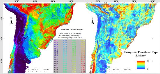
The Ecosystem Functional Types map presented in Figure 2 shows a synthetic characterization of spatial patterns of ecosystem functioning in temperate South America for the 2001–2008 period. Almost all possible combinations of EVI_mean, EVI_sCV and DMAX were identified in the study area. On average, most ecosystems showed EVI maxima in autumn and summer. EFTs with summer maxima tended to have medium-to-low productivity and high seasonality, while EFTs with autumn and spring maxima showed most of the possible combinations of productivity and seasonality. EFTs with EVI maxima during winter tended to exhibit either very low or very high productivity with very low seasonality values. The definition and coding of EFTs allow for an ecological interpretation of the legend in terms of the three EVI metrics related to productivity (EVI_Mean), seasonality (EVI_sCV) and phenology (DMAX). The greatest EVI_Mean (D) was reached in the Alto Paraná Atlantic Forests and in the Southwestern Amazonian Moist Forests. All spatial references in this article are based upon the WWF Ecoregions Map of the World [67]. The lowest EVI_Mean (A) occurred in the Atacama-Sechura Deserts, in the Central Andean Dry Puna and in some central areas of the Patagonian Steppe. The EVI_sCV was relatively low (c, d) throughout the study area. The greatest seasonality (a) occurred in the highest altitudes of: (1) the southern Andes (highest parts of the Valdivian Temperate Forests) and (2) the northern Andes (Bolivian Montane Dry Forest and Central Andean Wet Puna). High seasonality (a, b) is also found in agricultural lands of central and northwestern Argentina (across the Espinal and Dry Chaco) and eastern Brazil (across the Caatinga and Atlantic Dry Forests). The lowest seasonality (d) was observed in both: (1) the driest ecoregions, like the Atacama Desert and the Patagonian Steppe and (2) in very humid ecoregions, like the Alto Paraná Atlantic Forests and the Southwestern Amazonian Moist Forests. The phenological indicator of the growing season, DMAX, showed that most areas of extratropical South America have summer (2) and autumn (3) EVI maxima. Spring (1) maxima were observed just in the southeastern half of the Humid Pampas and the Uruguayan Savanna. Winter (4) maxima are scarce and mainly occur in the northernmost Chilean Matorral and in the Southwestern Amazonian Moist Forests.
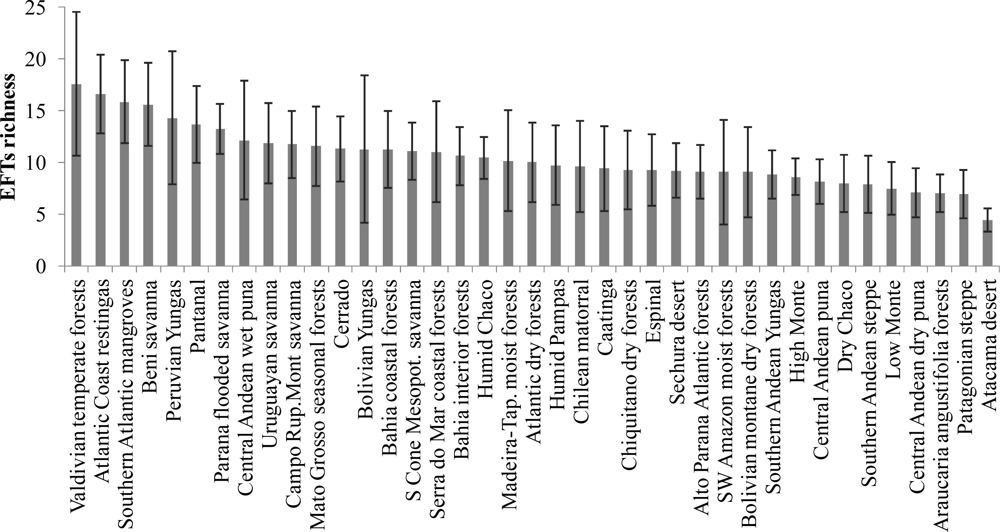
EFT richness was not evenly distributed across temperate South America, but showed contrasting and aggregated patterns across geographic features and ecoregions (Figures 3 and 4). EFT richness was locally increased by the presence of water bodies, along main river valleys and along the coastlines of Southern Brazil, Uruguay and Central-East Argentina (Buenos Aires province). The greatest EFT richness was observed in ecotones between the major vegetation types and ecoregions, such as in: (1) the ecotone of the Peruvian and Bolivian Yungas with the Central Andean Wet Punas and the Bolivian Montane Dry Forests, (2) the entire region of the Beni Savanna, (3) the ecotone between the Cerrado Woodlands and Savannas, the Matto Grosso Seasonal Forest, the Chiquitano Dry Forest and the Pantanal, and (4) the ecotone between the Chilean Matorral and the Valdivian Temperate Rainforest. The lowest values of EFT richness were reached mainly in drylands, such as the Atacama-Sechura Deserts, the Patagonian Steppe and the Southern Low Monte and the central regions of Dry Chaco and Espinal ecoregions. Relatively low values were also observed in the Araucaria Moist Forests and in areas of the Southwestern Amazonian Moist Forests close to the Andes.
3.2. Environmental and Human Controls of EFT Richness
As observed for species richness in the southern hemisphere [38], water availability, not energy, emerged as the main driver of EFT richness in natural ecosystems of temperate South America (Tables 1 and 2). Precipitation, distance to water bodies, frequency of wet days and percentage of the pixel occupied by water explained from 11 to 24% of the variability in the EFT richness. As precipitation values are mainly determined by geographic factors, the EFT richness pattern is correlated with regional climatic zones. However, the occurrence of water bodies, mainly rivers, increased EFT richness even in humid lands. Variables that combine both energy and water were also relevant, such as potential evapotranspiration and the seasonality of potential evapotranspiration and vapor pressure. This is particularly important in inlands, where there is low influence of oceans (e.g., Patagonian Steppe and Dry Chaco). Among the energy variables, only the diurnal temperature range and its seasonality show relatively low AIC and explain a deviance greater than 10%.
In anthropogenic systems, human land-use reduced the influence of environmental controls on the EFT richness. The most important variables explaining the spatial patterns of EFT richness in these systems were those related to human land-use and topography. Relief heterogeneity (CV_Alt) explained the greatest amount of variability, which illustrates how topography determines the range of possible human land-uses. The percentage of croplands and the spatial variability in human pressure were also relevant. Finally, the occurrence of water bodies also determined part of the variability of the EFT richness in anthropogenic systems.
In mixed environments, those with a mosaic of both natural and human-influenced ecosystems, the variance explained decreased in comparison with both natural and anthropogenic systems. Only precipitation and water-energy variables related to the seasonality of potential evapotranspiration and vapor pressure showed percentages of variance greater than 10% and relatively low AIC.
3.3. Sense of the Relationships between the EFT Richness and the Explanatory Variables
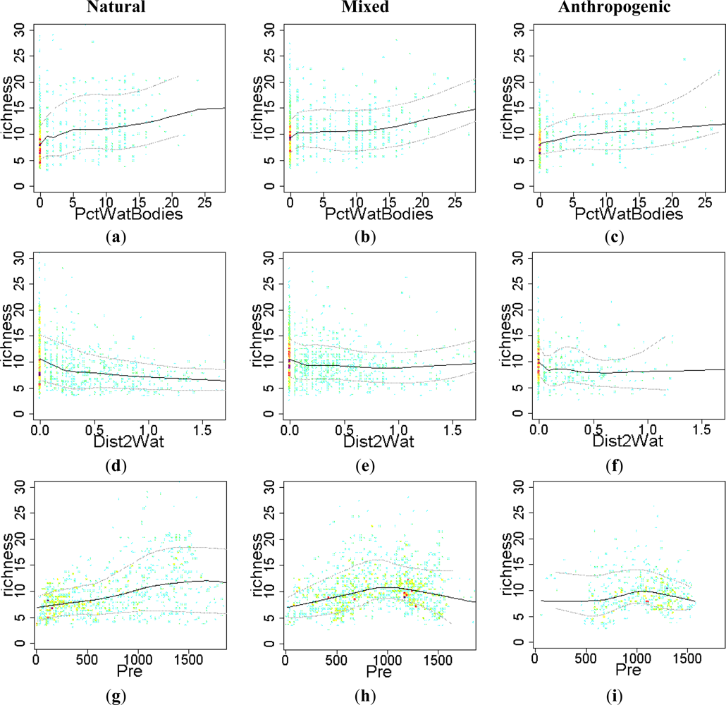
In general, water availability increased EFT richness (Figure 5), particularly in natural systems (Figure 5(a,d,g,j)). The positive effect of the percentage of water bodies was observed across the human-influence gradient, which agrees with the observed spatial pattern of high EFT richness along major rivers and water bodies in Figure 4. In natural ecosystems, the presence of surface water not only tended to increase EFT richness locally in those pixels, but also in neighbor pixels (Figure 5(d)), resulting in decreasing richness with increasing distance to water bodies. Clear examples of this effect are the great EFT richness values observed along major rivers (such as Parana, Uruguay, Río Negro and Río Colorado) and in flooded ecosystems (such as in Pantanal and Beni Savanna ecoregions). Precipitation and frequency of wet days showed similar positive effects on EFT richness, particularly in natural ecosystems, where they saturate with very humid conditions (over 1500 mm of precipitation, Figure 5(g,j)). In mixed and anthropogenic systems, precipitation and wet day frequency tended to increase EFT richness particularly in dry conditions, but the effect became negative in humid conditions (over 1,000–1,200 mm of rain).
Explanatory variables associated with both energy and water availability, such as potential evapotranspiration, tended to be negatively correlated with EFT richness (Figure 6(a–c)): the greater the mean annual potential evapotranspiration, the lower the EFT richness, particularly in natural ecosystems. On the other hand, low seasonality in either potential evapotranspiration or vapor pressure was associated with high EFT richness, particularly in natural and mixed systems (Figure 6(d,e,g,h)).
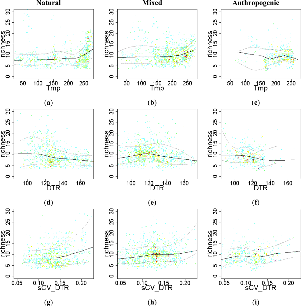
From the set of energy-related variables, only temperature showed a positive effect on EFT richness across natural and mixed ecosystems (Figure 7(a,b)). This positive effect of temperature on EFT richness was particularly noticeable in warmer locations (temperature greater than 20 °C). Increased diurnal temperature range had a negative effect on EFT richness (Figure 7(d)), while seasonal differences in the diurnal temperature range were positively related to EFT richness (Figure 7(g–i)).
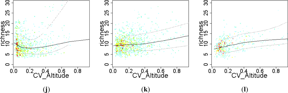
Relief heterogeneity showed a clear positive effect on EFT richness in human-influenced ecosystems (both anthropogenic and mixed, Figure 7(k,l)) and in natural ecosystems that occurred on irregular terrains (altitude coefficient of variation greater than 20%; Figure 7(j)). However, in natural ecosystems that occurred on smooth relief (up to a 10% of terrain altitude coefficients of variation), relief heterogeneity was negatively related to EFT richness (Figure 7(j)).
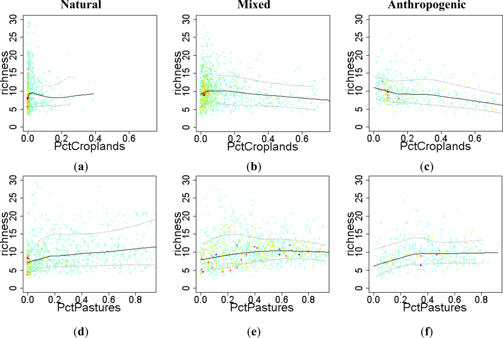
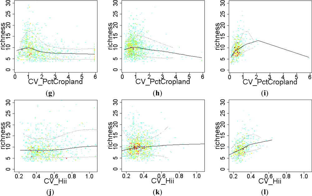
The effect of the percentage of area occupied by crops on EFT richness varied from being positive at the early stages of cropland expansion, to negative when croplands started to spread out and dominate the landscape (Figure 8(a–c)). The introduction of croplands in a natural landscape at very low densities, up to 5% of natural vegetation replaced by crops (0.05 in the graph), showed a positive relationship with EFT richness, (Figure 8(a,b)). However, replacing more than 10% of natural vegetation by crops had a clear negative effect on EFT richness (Figure 8(b,c)). In contrast to crops, pasture maintained a positive relationship with EFT richness in natural ecosystems both at low and high percentages of pastured land (Figure 8(d)). In mixed and anthropogenic systems, such a positive effect of pasture on EFT richness occurred, just up to 40% of the cell being occupied by pastures (Figure 8(e,f)). The effect on EFT richness of the spatial variability in the percentage of croplands or in the human influence index was unclear (Figure 8(g–k)). Only in anthropogenic areas, the spatial heterogeneity in human influence within a cell showed a positive relationship with EFT richness (Figure 8(l)).
Moran’s I correlograms show significant spatial autocorrelation at the finest scale of analysis in the residuals of all models (Figure A1). However, autocorrelation strongly decreases within the first 200 km and remains below 0.1 at 300 km and greater. This is indicative of the relatively high levels of unexplained deviance that remain after fitting very simple models (of just one single explanatory variable) across a very heterogeneous region. It is interesting to note that anthropogenic systems show the steepest decreases in spatial autocorrelation with distance and mixed systems the most gradual.
4. Discussion
The three components of biodiversity (composition, structure and function) at all levels of organization determine and, in fact, constitute the biodiversity of an area and should be considered in conservation efforts [1]. Recently, the ecosystem functioning dimension of biodiversity has gained attention [3] given that global change effects on biodiversity are particularly noticeable at the ecosystem level [4] and have a faster influence on functional than on structural or compositional characteristics of ecosystems [5,6]. Thus, understanding how environmental and human factors operate on the functional dimension of biodiversity at different scales is critical for sustaining and enhancing the Earth’s ecosystems. Here, we characterize the spatial patterns of functional diversity at the ecosystem level and provide evidence for the main controls of ecosystem functional diversity in temperate South America. Satellite-derived time-series of the Enhanced Vegetation Index were used to quantify functional diversity at the ecosystem level through the identification of Ecosystem Functional Types, defined here as ecological entities that have similar properties and dynamics of primary production. Numerous studies have successfully evaluated the use of remotely-sensed spectral diversity to estimate species richness [79–83] and species beta-diversity [84,85]. Our study focused not on estimating the diversity of species composition or turn-over, but on assessing the diversity of ecosystem functioning.
Our definition of EFTs is based on estimators of the seasonal dynamics of carbon gains, but remote sensing may provide additional functional variables to complement ecosystem functioning descriptions at the same and different spatial and temporal resolutions [3,86,87]. For instance, Fernández et al.[23] showed how adding shortwave albedo and surface temperature, two variables closely linked to the exchange of energy in ecosystems, to carbon gains descriptors helped to complement the ecosystem functioning characterization at more detailed spatial resolutions. Our EFT identification could have also been based on automatic algorithms (e.g., ISODATA or k-means, [8,23]) instead of on fixed-limits between classes. However, when we assessed automatic unsupervised classifications with the three EVI traits, continuity in the final map was very low and biological interpretability of the classes was not straightforward. In addition, the limits between classes when using automatic algorithms change from year to year (since they depend on the input data). In contrast, once defined, our fixed-limit classification approach allows for inter-annual comparisons, since we apply the same limits between classes in each year.
EFT richness in temperate South America showed contrasting and aggregated patterns across geographic features and ecoregions, indicating that major controls of ecosystem functional diversity correlate with regional climatic zones. EFT richness patterns showed both the effect of large-scale geographical patterns, such as mountain ranges or flatlands and local scale features, such as rivers or lagoons. The presence and proximity of surface water along the main river valleys and Atlantic coastal lagoons locally increased EFT richness. Ecotones between major vegetation types and ecoregions also showed a local increase in EFT richness. This positive effect of ecotones on ecosystem functional diversity may play an important role in explaining regional beta-diversity patterns, since biome edges have been highlighted as global hotspots of congruence of high beta-diversity values for birds, amphibians and mammals [88].
As was found to explain species richness patterns in the subtropical and warm temperate zones [38], water variables were revealed as the strongest control of EFT richness in natural and mixed systems, followed by water-energy balance variables. In addition, since the hydrological budget and the variability in temperature are the main driving factors that determine major vegetation types at global and regional scales [89,90], it was expected that the existence of biotic controls on EFT richness would be derived from the structure and composition of plant biodiversity. Thus, we found that ecoregions with the highest ecosystem functional diversity corresponded to humid forests and flooded ecosystems, particularly those that have a mosaic of forests and savannas with trees and shrubs [91,92]. However, ecoregions corresponding to grasslands and drylands showed the lowest EFT richness, which may be related to the role of frosts and droughts in constraining the diversity of plant species [37] and, hence, of ecosystem functional diversity.
Human impacts on the landscape largely remove the influence of these environmental controls of EFT richness. Our analyses across large anthropogenic areas of South America provide additional evidence as to how human forces currently outweigh environmental drivers of ecosystem processes and biodiversity [58]. Variables related to livestock systems do not show significant influences on EFT richness. This lack of influence could be associated with the similarity of vegetation structure and functioning between pastures and the vegetation type replaced (steppes, grasslands, dry forests or savannas). Such differences may become important for pastures derived from the clearing of humid forests. In contrast, the introduction of croplands and human developments clearly modified functional patterns of the landscape, with stronger effects on the seasonality of carbon gains than on total gains [93]. While low densities of croplands have positive effects on EFT richness, extending the coverage of croplands to over 5% of the land surface decreased ecosystem functional diversity. On the other hand, the increase of the spatial heterogeneity of different land-covers introduced by human land-uses, a main feature of anthropogenic systems [58], increased EFT richness. In this sense, the conversion of natural areas into croplands would only increase EFT richness if it increased the landscape spatial heterogeneity, which often occurs during the initial stages of cropland expansion. Another interesting point is the positive effect that pasture had on EFT richness, mainly at less than 20% of pastured area in natural ecosystems and 40% of pastured area in mixed and anthropogenic ecosystems.
Since ecosystems are spatially structured, it is expected that environmental variables would show high levels of spatial autocorrelation [78]. In our analyses, anthropogenic systems showed the smallest residuals with regard to spatial autocorrelation. This reinforces our result that human influence has a greater effect on EFT richness in anthropogenic systems than other environmental variables have in natural or mixed systems, where the major drivers of EFT richness correspond to the regional climate. Previous studies also showed how human land-use strongly decouples the spatial pattern of ecosystem functions from that of energy and water climate variables [94]. In any case, the presence of spatial autocorrelation in the residuals after model fitting indicates the existence of systematic spatial patterns in data quality or of missing variables (e.g., [51,95,96]). For this reason, one should be cautious in interpreting those models that have both low explanatory power and high spatial autocorrelation in the residuals.
5. Conclusions
As far as we know, this is the first study that evaluates the main controls of functional diversity at the ecosystem level. Satellite-derived time-series of the Enhanced Vegetation Index were used to quantify the spatial patterns of ecosystem functional diversity in temperate South America through the identification of 64 Ecosystem Functional Types (EFTs), defined as ecological entities that have similar properties and dynamics of primary production. Our models of the relationship between EFT diversity and environmental variables are incomplete representations of factors influencing regional scale patterns of ecosystem functional diversity. However, our models highlight how the main drivers of EFT richness agree with those found for species richness. The models show that meaningful proportions of the variance in EFT richness can be accounted for by the single-effects of climate (up to 24% explained by precipitation and 22% by potential evapotranspiration in natural environments), relief (20% explained by altitude coefficient of variation in anthropogenic environments) or human-influence (15% explained by the percentage of croplands in the landscape). Going back to our guiding hypotheses, we found general support for the consideration that water availability (24% variance explained by precipitation, 22% by distance to water and 16% by wet-days frequency) is the main limiting factor for EFT richness in natural environments of temperate South-America. It is followed by mixed water-energy (22% explained by potential evapotranspiration) and energy variables (13% explained by diurnal temperature range) (Hypotheses H2a, H2b, H2c). Contrary to our expectations (H5), EFT richness is not strongly controlled by topographic roughness in natural environments (only 2% of explained deviance). However, in anthropogenic landscapes, the effects of both energy and water-related climate variables on EFT richness is largely removed (non-significant values of explained deviance), leaving human land-use (up to 16% deviance explained by the spatial variability of the percentage of croplands), relief heterogeneity (20% explained by altitude coefficient of variation) and the presence of surface water bodies (13% of explained deviance) as the main drivers of EFT richness. Temporal variability of climate did not show a clear effect on EFT richness (H3). While diurnal temperature range showed a negative relationship with EFT richness in natural environments, seasonality of the diurnal temperature range showed a weak positive effect. In contrast, seasonality of mixed water-energy variables (potential evapotranspiration and vapor pressure) showed a negative effect on EFT richness. In human influenced environments, the introduction of human land-use has a positive effect on EFT richness at low rates of human pressure, but it switches to a negative effect at large or severe rates of human intervention (H4). For future work, our remote sensing approach to quantify functional diversity at the ecosystem level opens the possibility to evaluate how species diversity relates to ecosystem functional diversity and to determining if species and functional diversity show similar responses to environmental and human controls.
Acknowledgments
To Hugo Berbery and Esteban Jobbágy for their funding and help. Funds were given by the Inter-American Institute for Global Change Research (CRN II 2031 & 2094) under the US NSF Grant GEO-0452325, the postdoctoral program of the Spanish Ministry of Education to D. Alcaraz-Segura, FEDER Funds, Junta de Andalucía (Projects GLOCHARID & SEGALERT P09–RNM-5048), Ministerio de Ciencia e Innovación (Project CGL2010-22314), Fundación MAPFRE 2008 R+D project, Ecología de Zonas Áridas Research Group, University of Almería, CONICET, FONCYT and SNAP (Dirección Nacional de Medio Ambiente, Uruguay).
References
- Noss, R.F. Indicators for monitoring biodiversity—A hierarchical approach. Conserv. Biol 1990, 4, 355–364. [Google Scholar]
- Callicott, J.B.; Crowder, L.B.; Mumford, K. Current normative concepts in conservation. Conserv. Biol 1999, 13, 22–35. [Google Scholar]
- Cabello, J.; Fernández, N.; Alcaraz-Segura, D.; Oyonarte, C.; Piñeiro, G.; Altesor, A.; Delibes, M.; Paruelo, J. The ecosystem functioning dimension in conservation: Insights from remote sensing. Biodiver. Conserv 2012, 21, 3287–3305. [Google Scholar]
- Vitousek, P.M. Beyond global warming: Ecology and global change. Ecology 1994, 75, 1861–1876. [Google Scholar]
- Milchunas, D.G.; Lauenroth, W.K. Inertia in plant community structure: State changes after cessation of nutrient enrichment stress. Ecol. Appl 1995, 5, 1195–2005. [Google Scholar]
- McNaughton, S.; Oesterheld, M.; Frank, D.; Williams, K. Ecosystem-level patterns of primary productivity and herbivory in terrestrial habitats. Nature 1989, 341, 142–144. [Google Scholar]
- Valentini, R.; Baldocchi, D.D.; Tenhunen, J.D.; Kabat, P. Ecological Controls on Land-Surface Atmospheric Interactions. In Integrating Hydrology, Ecosystem Dynamics and Biogeochemistry in Complex Landscapes; John Wiley & Sons: Berlin, Germany, 1999; pp. 105–116. [Google Scholar]
- Paruelo, J.M.; Jobbagy, E.G.; Sala, O.E. Current distribution of ecosystem functional types in temperate South America. Ecosystems 2001, 4, 683–698. [Google Scholar]
- Shugart, H.H.; Smith, T.M.; Woodward, F.I. Plant and Ecosystem Functional Types. In Plant Functional Types. Their Relevance to Ecosystem Properties and Global Change; Cambridge University Press: Cambridge, UK, 1997; pp. 20–45. [Google Scholar]
- Díaz, S.; Cabido, M. Plant functional types and ecosystem function in relation to global change. J. Veg. Sci 1997, 8, 463–474. [Google Scholar]
- Scholes, R.J.; Pickett, G.; Ellery, W.N.; Blackmore, A.C.; Smith, T.M.; Shugart, H.H.; Woodward, F.I. Plant Functional Types in African Savannas and Grasslands. In Plant Functional Types. Their Relevance to Ecosystem Properties and Global Change; Cambridge University Press: Cambridge, UK, 1997; pp. 255–268. [Google Scholar]
- Walker, B.H.; Smith, T.M.; Shugart, H.H.; Woodward, F.I. Functional Types in Non-Equilibrium Ecosystems. In Plant Functional Types. Their Relevance to Ecosystem Properties and Global Change; Cambridge University Press: Cambridge, UK, 1997; pp. 91–103. [Google Scholar]
- Aber, J.D.; Burke, I.C.; Acock, B.; Bugmann, H.K.M.; Kabat, P.; Menaut, J.C.; Noble, I.R.; Reynolds, J.F.; Steffen, W.L.; Wu, J.; Tenhunen, J.D. Group Report: Hydrological and Biogeochemical Processes in Complex Landscapes—What Is the Role of Temporal and Spatial Ecosystem Dynamics? In Integrating Hydrology, Ecosystem Dynamics and Biogeochemistry in Complex Landscapes; John Wiley & Sons: Berlin, Germany, 1999; pp. 335–356. [Google Scholar]
- Bonan, G.B.; Levis, S.; Kergoat, L.; Oleson, K.W. Landscapes as patches of plant functional types: An integrating concept for climate and ecosystem models. Glob. Biogeochem. Cy. 2002. [Google Scholar] [CrossRef]
- Duckworth, J.C.; Kent, M.; Ramsay, P.M. Plant functional types: An alternative to taxonomic plant community description in biogeography? Progr. Phys. Geogr 2000, 24, 515–542. [Google Scholar]
- Bret-Harte, M.S.; Mack, M.C.; Goldsmith, G.R.; Sloan, D.B.; DeMarco, J.; Shaver, G.R.; Ray, P.M.; Biesinger, Z.; Chapin, F.S. Plant functional types do not predict biomass responses to removal and fertilization in Alaskan tussock tundra. J. Ecol 2008, 96, 713–726. [Google Scholar]
- Lavorel, S.; Díaz, S.; Cornelissen, J.; Garnier, E.; Harrison, S.; McIntyre, S.; Pausas, J.; Pérez-Harguindeguy, N.; Roumet, C.; Urcelay, C. Plant Functional Types: Are We Getting Any Closer to the Holy Grail? In Terrestrial Ecosystems in a Changing World; Canadell, J.G., Pataki, D.E., Pitelka, L.F., Eds.; Springer: Berlin/Heidelberg, Germany/New York, NY, USA, 2007; pp. 149–164. [Google Scholar]
- Wright, J.P.; Naeem, S.; Hector, A.; Lehman, C.; Reich, P.B.; Schmid, B.; Tilman, D. Conventional functional classification schemes underestimate the relationship with ecosystem functioning. Ecol. Lett 2006, 9, 111–120. [Google Scholar]
- Soriano, A.; Paruelo, J.M. Biozones: Vegetation units defined by functional characters identifiable with the aid of satellite sensor images. Glob. Ecol. Biogeogr. Lett 1992, 2, 82–89. [Google Scholar]
- Stow, D.; Daeschner, S.; Boynton, W.; Hope, A. Arctic tundra functional types by classification of single-date and AVHRR bi-weekly NDVI composite datasets. Int. J. Remote Sens 2000, 21, 1773–1779. [Google Scholar]
- Alcaraz-Segura, D.; Paruelo, J.M.; Cabello, J. Identification of current ecosystem functional types in the Iberian Peninsula. Glob. Ecol. Biogeogr 2006, 15, 200–212. [Google Scholar]
- Piñeiro, G.; Alcaraz-Segura, D.; Paruelo, J.M.; Oyonarte, C.; Guerschman, J.P.; Escribano, P.; Cabello, J. A Functional Classification of Natural and Human-Modified Areas of “Cabo de Gata”, Spain, Based on Landsat TM Data. Proceedings of 29th International Symposium on Remote Sensing of Environment, Buenos Aires, Argentina, 8–12 April 2002.
- Fernández, N.; Paruelo, J.M.; Delibes, M. Ecosystem functioning of protected and altered Mediterranean environments: A remote sensing classification in Doñana, Spain. Remote Sens. Environ 2010, 114, 211–220. [Google Scholar]
- Pérez-Hoyos, A.; Martínez, B.; Gilabert, M.A.; García-Haro, F.J. A multi-temporal analysis of vegetation dynamics in the Iberian peninsula using MODIS-NDVI data. EARSeL eProc 2010, 9, 22–30. [Google Scholar]
- Martínez, B.; Gilabert, M.A. Vegetation dynamics from NDVI time series analysis using the wavelet transform. Remote Sens. Environ 2009, 113, 1823–1842. [Google Scholar]
- Stoyanova, J.S. Bioclimatic Concept for Assessment of Atmosphere and Forest Land-Cover Coupling at a Regional Scale. Proceedings of 29th International Conference on Alpine Meteorology, Chambéry, France, 4–8 June 2007.
- Alcaraz-Segura, D.; Berbery, E.H.; Lee, S.-J.; Paruelo, J.M. Use of ecosystem functional types to represent the interannual variability of vegetation biophysical properties in regional models. CLIVAR Exchanges 2011, 17, 23–27. [Google Scholar]
- Muller, O.; Berbery, E.H.; Alcaraz-Segura, D. The Drought Interest Group: Using Ecosystem Functional Types as Lower Boundary Conditions in Simulations of Droughts in Southern South America. Proceedings of WCRP Open Science Conference. Climate Research in Service to Society, Denver, CO, USA, 24–28 October 2011; p. C39 TH98A.
- Berbery, E.H.; Alcaraz-Segura, D.; Muller, O. Time-Varying Biophysical Properties of Terrestrial Ecosystems: Their Use in Regional Climate Modeling. Proceedings of WCRP Open Science Conference. Climate Research in Service to Society, Denver, CO, USA, 24–28 October 2011; p. C10 M36A.
- Karlsen, S.R.; Elvebakk, A.; Høgda, K.A.; Johansen, B. Satellite-based mapping of the growing season and bioclimatic zones in Fennoscandia. Glob. Ecol. Biogeogr 2006, 15, 416–430. [Google Scholar]
- Azzali, S.; Menenti, M. Mapping isogrowth zones on continental scale using temporal Fourier analysis of AVHRR-NDVI data. Int. J. Appl. Earth Obs. Geoinf 1999, 1, 9–20. [Google Scholar]
- Azzali, S.; Menenti, M. Mapping vegetation-soil-climate complexes in southern Africa using temporal Fourier analysis of NOAA-AVHRR NDVI data. Int. J. Remote Sens 2000, 21, 973–996. [Google Scholar]
- Duro, D.; Coops, N.C.; Wulder, M.A.; Han, T. Development of a large area biodiversity monitoring system driven by remote sensing. Progr. Phys. Geogr 2007, 31, 235–260. [Google Scholar]
- Mildrexler, D.J.; Zhao, M.S.; Heinsch, F.A.; Running, S.W. A new satellite-based methodology for continental-scale disturbance detection. Ecol. Appl 2007, 17, 235–250. [Google Scholar]
- Sobrino, J.A.; Julien, Y.; Morales, L. Multitemporal analysis of PAL images for the study of land cover dynamics in South America. Glob. Planet. Change 2006, 51, 172–180. [Google Scholar]
- Geerken, R.A. An algorithm to classify and monitor seasonal variations in vegetation phenologies and their inter-annual change. ISPRS J. Photogramm 2009, 64, 422–431. [Google Scholar]
- Kreft, H.; Jetz, W. Global patterns and determinants of vascular plant diversity. Proc. Natl. Acad. Sci. USA 2007, 104, 5925–5930. [Google Scholar]
- Hawkins, B.A.; Field, R.; Cornell, H.V.; Currie, D.J.; Guegan, J.F.; Kaufman, D.M.; Kerr, J.T.; Mittelbach, G.G.; Oberdorff, T.; O’Brien, E.M.; Porter, E.E.; Turner, J.R.G. Energy, water and broad-scale geographic patterns of species richness. Ecology 2003, 84, 3105–3117. [Google Scholar]
- Hawkins, B.A. Are we making progress toward understanding the global diversity gradient? Basic Appl. Ecol 2004, 5, 1–3. [Google Scholar]
- Hawkins, B.A.; McCain, C.M.; Davies, T.J.; Buckley, L.B.; Anacker, B.L.; Cornell, H.V.; Damschen, E.I.; Grytnes, J.-A.; Harrison, S.; Holt, R.D.; et al. Different evolutionary histories underlie congruent species richness gradients of birds and mammals. J. Biogeogr 2012, 39, 825–841. [Google Scholar]
- Gaston, K.J. Global patterns in biodiversity. Nature 2000, 405, 220–227. [Google Scholar]
- Cadena, C.D.; Kozak, K.H.; Gómez, J.P.; Parra, J.L.; McCain, C.M.; Bowie, R.C.K.; Carnaval, A.C.; Moritz, C.; Rahbek, C.; Roberts, T.E.; et al. Latitude, elevational climatic zonation and speciation in New World vertebrates. Proc. Roy. Soc. B: Biol. Sci 2012, 279, 194–201. [Google Scholar]
- Gould, W. Remote sensing of vegetation, plant species richness and regional biodiversity hotspots. Ecol. Appl 2000, 10, 1861–1870. [Google Scholar]
- Kerr, J.T.; Ostrovsky, M. From space to species: Ecological applications for remote sensing. Trend. Ecol. Evol 2003, 18, 299–305. [Google Scholar]
- Buchanan, G.; Pearce-Higgins, J.; Grant, M.; Robertson, D.; Waterhouse, T. Characterization of moorland vegetation and the prediction of bird abundance using remote sensing. J. Biogeogr 2005, 32, 697–707. [Google Scholar]
- Innes, J.L.; Koch, B. Forest biodiversity and its assessment by remote sensing. Glob. Ecol. Biogeogr 1998, 7, 397–419. [Google Scholar]
- Turner, W.; Spector, S.; Gardiner, N.; Fladeland, M.; Sterling, E.; Steininger, M. Remote sensing for biodiversity science and conservation. Trend. Ecol. Evol 2003, 18, 306–314. [Google Scholar]
- Leyequien, E.; Verrelst, J.; Slot, M.; Schaepman-Strub, G.; Heitkonig, I.M.A.; Skidmore, A. Capturing the fugitive: Applying remote sensing to terrestrial animal distribution and diversity. Int. J. Appl. Earth Obs. Geoinf 2007, 9, 1–20. [Google Scholar]
- Wiens, J.; Sutter, R.; Anderson, M.; Blanchard, J.; Barnett, A.; Aguilar-Amuchastegui, N.; Avery, C.; Laine, S. Selecting and conserving lands for biodiversity: The role of remote sensing. Remote Sens. Environ 2009, 113, 1370–1381. [Google Scholar]
- Goetz, S.; Steinberg, D.; Dubayah, R.; Blair, B. Laser remote sensing of canopy habitat heterogeneity as a predictor of bird species richness in an eastern temperate forest, USA. Remote Sens. Environ 2007, 108, 254–263. [Google Scholar]
- Whittaker, R.J.; Nogués-Bravo, D.; Araújo, M.B. Geographical gradients of species richness: A test of the water-energy conjecture of Hawkins et al. (2003) using European data for five taxa. Glob. Ecol. Biogeogr 2007, 16, 76–89. [Google Scholar]
- Carnaval, A.C.; Hickerson, M.J.; Haddad, C.F.B.; Rodrigues, M.T.; Moritz, C. Stability predicts genetic diversity in the Brazilian Atlantic forest hotspot. Science 2009, 323, 785–789. [Google Scholar]
- Kiessling, W. Long-term relationships between ecological stability and biodiversity in Phanerozoic reefs. Nature 2005, 433, 410–413. [Google Scholar]
- Tilman, D.; Reich, P.B.; Knops, J.M.H. Biodiversity and ecosystem stability in a decade-long grassland experiment. Nature 2006, 441, 629–632. [Google Scholar]
- Benton, T.G.; Vickery, J.A.; Wilson, J.D. Farmland biodiversity: Is habitat heterogeneity the key? Trends Ecol. Evol 2003, 18, 182–188. [Google Scholar]
- Burnett, M.R.; August, P.V.; Brown, J.H., Jr.; Killingbeck, K.T. The influence of geomorphological heterogeneity on biodiversity I. A patch-scale perspective. Conserv. Biol 1998, 12, 363–370. [Google Scholar]
- Nichols, W.F.; Killingbeck, K.T.; August, P.V. The influence of geomorphological heterogeneity on Biodiversity II. A Landscape Perspective. Conserv. Biol 1998, 12, 371–379. [Google Scholar]
- Ellis, E.C.; Ramankutty, N. Putting people in the map: Anthropogenic biomes of the world. Front. Ecol. Environ 2007, 6, 439–447. [Google Scholar]
- Medan, D.; Torretta, J.P.; Hodara, K.; de la Fuente, E.B.; Montaldo, N.H. Effects of agriculture expansion and intensification on the vertebrate and invertebrate diversity in the Pampas of Argentina. Biodivers. Conserv 2011, 20, 3077–3100. [Google Scholar]
- Cerezo, A.; Conde, M.C.; Poggio, S.L. Pasture area and landscape heterogeneity are key determinants of bird diversity in intensively managed farmland. Biodivers. Conserv 2011, 20, 2649–2667. [Google Scholar]
- Jauni, M.; Hyvönen, T. Positive diversity-invasibility relationships across multiple scales in Finnish agricultural habitats. Biol. Invasions 2011, 14, 1379–1391. [Google Scholar]
- Tognetti, P.M.; Chaneton, E.J.; Omacini, M.; Trebino, H.J.; León, R.J.C. Exotic vs. native plant dominance over 20 years of old-field succession on set-aside farmland in Argentina. Biol. Conserv 2010, 143, 2494–2503. [Google Scholar]
- Poggio, S.L.; Chaneton, E.J.; Ghersa, C.M. Landscape complexity differentially affects alpha, beta and gamma diversities of plants occurring in fencerows and crop fields. Biol. Conserv 2010, 143, 2477–2486. [Google Scholar]
- Larsen, T.H. Upslope range shifts of andean dung beetles in response to deforestation: compounding and confounding effects of microclimatic change. Biotropica 2012, 44, 82–89. [Google Scholar]
- Strassburg, B.B.N.; Rodrigues, A.S.L.; Gusti, M.; Balmford, A.; Fritz, S.; Obersteiner, M.; Turner, R.K.; Brooks, T.M. Impacts of incentives to reduce emissions from deforestation on global species extinctions. Nature Clim. Change 2012, 2, 350–355. [Google Scholar]
- Kottek, M.; Grieser, J.; Beck, C.; Rudolf, B.; Rubel, F. World Map of the Koppen-Geiger climate classification updated. Meteorologische Zeitschrift 2006, 15, 259–263. [Google Scholar]
- Olson, D.M.; Dinerstein, E.; Wikramanayake, E.D.; Burgess, N.D.; Powell, G.V.N.; Underwood, E.C.; D’Amico, J.A.; Itoua, I.; Strand, H.E.; Morrison, J.C.; et al. Terrestrial ecoregions of the world: A new map of life on Earth. BioScience 2001, 51, 933–938. [Google Scholar]
- Sanderson, E.W.; Jaiteh, M.; Levy, M.A.; Redford, K.H.; Wannebo, A.V.; Woolmer, G. The human footprint and the last of the wild. BioScience 2002, 52, 891–904. [Google Scholar]
- Alcaraz-Segura, D.; Paruelo, J.M.; Cabello, J. Baseline characterization of major Iberian vegetation types based on the NDVI dynamics. Plant Ecol 2009, 202, 13–29. [Google Scholar]
- Virginia, R.A.; Wall, D.H.; Levin, S.A. Principles of Ecosystem Function. In Encyclopedia of Biodiversity; Academic Press: San Diego, CA, USA, 2001; pp. 345–352. [Google Scholar]
- Pettorelli, N.; Vik, J.O.; Mysterud, A.; Gaillard, J.M.; Tucker, C.J.; Stenseth, N.C. Using the satellite-derived NDVI to assess ecological responses to environmental change. Trend. Ecol. Evol 2005, 20, 503–510. [Google Scholar]
- Paruelo, J.M.; Epstein, H.E.; Lauenroth, W.K.; Burke, I.C. ANPP estimates from NDVI for the Central Grassland Region of the United States. Ecology 1997, 78, 953–958. [Google Scholar]
- Monfreda, C.; Ramankutty, N.; Foley, J.A. Farming the planet: 2. Geographic distribution of crop areas, yields, physiological types and net primary production in the year 2000. Glob. Biogeochem. Cy 2008, 22, 1–19. [Google Scholar]
- Ramankutty, N.; Evan, A.T.; Monfreda, C.; Foley, J.A. Farming the planet: 1. Geographic distribution of global agricultural lands in the year 2000. Glob. Biogeochem. Cy 2008, 22, 1–19. [Google Scholar]
- Lehner, B.; Verdin, K.; Jarvis, A. HydroSHEDS Technical Documentation; Version 1.0; World Wildlife Fund US: Washington, DC, USA, 2008. [Google Scholar]
- Crawley, M.J. GLIM for Ecologists; Blackwell Scientific Publications: Oxford, UK, 1993. [Google Scholar]
- Ricci, V. Fitting Distributions with R; CRAN: Vienna, Austria, 2005; p. 24. [Google Scholar]
- Legendre, P.; Legendre, L. Numerical Ecology: Developments in Environmental Modelling; Elsevier Publishers: Amsterdam, The Netherlands, 1998. [Google Scholar]
- Higgins, M.A.; Asner, G.P.; Perez, E.; Elespuru, N.; Tuomisto, H.; Ruokolainen, K.; Alonso, A. Use of Landsat and SRTM data to detect broad-scale biodiversity patterns in Northwestern Amazonia. Remote Sens 2012, 4, 2401–2418. [Google Scholar]
- Nagendra, H.; Rocchini, D.; Ghate, R.; Sharma, B.; Pareeth, S. Assessing plant diversity in a dry tropical forest: Comparing the utility of Landsat and IKONOS satellite images. Remote Sens 2010, 2, 478–496. [Google Scholar]
- Leutner, B.F.; Reineking, B.; Müller, J.; Bachmann, M.; Beierkuhnlein, C.; Dech, S.; Wegmann, M. Modelling forest α-diversity and floristic composition—On the added value of LiDAR plus hyperspectral remote sensing. Remote Sens 2012, 4, 2818–2845. [Google Scholar]
- Rocchini, D.; Balkenhol, N.; Carter, G.A.; Foody, G.M.; Gillespie, T.W.; He, K.S.; Kark, S.; Levin, N.; Lucas, K.; Luoto, M. Remotely sensed spectral heterogeneity as a proxy of species diversity: recent advances and open challenges. Ecol. Inform 2010, 5, 318–329. [Google Scholar]
- Rocchini, D.; McGlinn, D.; Ricotta, C.; Neteler, M.; Wohlgemuth, T. Landscape complexity and spatial scale influence the relationship between remotely sensed spectral diversity and survey-based plant species richness. J. Veg. Sci 2011, 22, 688–698. [Google Scholar]
- Rocchini, D. Commentary on Krishnaswamy et al.—Quantifying and mapping biodiversity and ecosystem services: Utility of a multi-season NDVI based Mahalanobis distance surrogate. Remote Sens. Environ 2009, 113, 904–906. [Google Scholar]
- Krishnaswamy, J.; Bawa, K.S.; Ganeshaiah, K.N.; Kiran, M.C. Quantifying and mapping biodiversity and ecosystem services: Utility of a multi-season NDVI based Mahalanobis distance surrogate. Remote Sens. Environ 2009, 113, 857–867. [Google Scholar]
- Eisele, A.; Lau, I.; Hewson, R.; Carter, D.; Wheaton, B.; Ong, C.; Cudahy, T.J.; Chabrillat, S.; Kaufmann, H. Applicability of the thermal infrared spectral region for the prediction of soil properties across semi-arid agricultural landscapes. Remote Sens 2012, 4, 3265–3286. [Google Scholar]
- Nemani, R.R.; Running, S.W. Land cover characterization using multitemporal red, near-IR and thermal-IR data from NOAA/AVHRR. Ecol. Appl 1997, 7, 79–90. [Google Scholar]
- McKnight, M.W.; White, P.S.; McDonald, R.I.; Lamoreux, J.F.; Sechrest, W.; Ridgely, R.S.; Stuart, S.N. Putting beta-diversity on the map: Broad-scale congruence and coincidence in the extremes. PLoS Biol 2007, 5, e272. [Google Scholar]
- Woodward, F.I.; Williams, B.G. Climate and plant distribution at global and local scales. Plant Ecolog 1987, 69, 189–197. [Google Scholar]
- Holdridge, L.R. Determination of world plant formations from simple climatic data. Science 1947, 105, 367. [Google Scholar]
- Archibold, O.W. Ecology of World Vegetation; Chapman & Hall Ltd: London, UK, 1995. [Google Scholar]
- Morrone, J.J. Biogeografía de América Latina y el Caribe; M&T–Manuales & Tesis SEA: Zaragoza, Spain, 2001. [Google Scholar]
- Volante, J.N.; Alcaraz-Segura, D.; Mosciaro, M.J.; Viglizzo, E.F.; Paruelo, J.M. Ecosystem functional changes associated with land clearing in NW Argentina. Agric. Ecosyst. Environ 2011, 154, 12–22. [Google Scholar]
- Liras, E.; Cabello, J.; Alcaraz-Segura, D.; Paruelo, J.; Maestre, F.T. Patrones Espaciales del Funcionamiento de los Ecosistemas: Efectos del Cambio en la Cobertura y el Uso del Suelo. In Analisis Espacial en Ecología, Métodos y Aplicaciones; Asociación Española de Ecología Terrestre: Alicante, 2008; pp. 717–730. [Google Scholar]
- Segurado, P.; Araújo, M.B.; Kunin, W.E. Consequences of spatial autocorrelation for niche-based models. J. Appl. Ecol 2006, 43, 433–444. [Google Scholar]
- Diniz-Filho, J.A.F.; Bini, L.M.; Hawkins, B.A. Spatial autocorrelation and red herrings in geographical ecology. Glob. Ecol. Biogeogr 2003, 12, 53–64. [Google Scholar]
Appendix
Figure A1.
Moran’s I correlograms of the residuals obtained after fitting Generalized Linear Models (GLM) models to the relationship between EFT richness and different environmental variables using first (circles) and second (triangles) degree polynomials. Relationships were compared across a gradient of Human Influence Index (HII): Natural ecosystems (in black; HII < 10), mixed (in blue; 10 < HII < 20) and anthropogenic systems (in red; HII > 20). Significant Moran’s I values (p < 0.05; 100 resamples) are shown as solid symbols. (Same order as in Table 1).
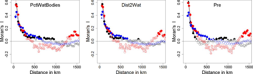


Figure 1.
Study area showing the World Wildlife Foundation Ecoregions map of South America [67].
Figure 1.
Study area showing the World Wildlife Foundation Ecoregions map of South America [67].
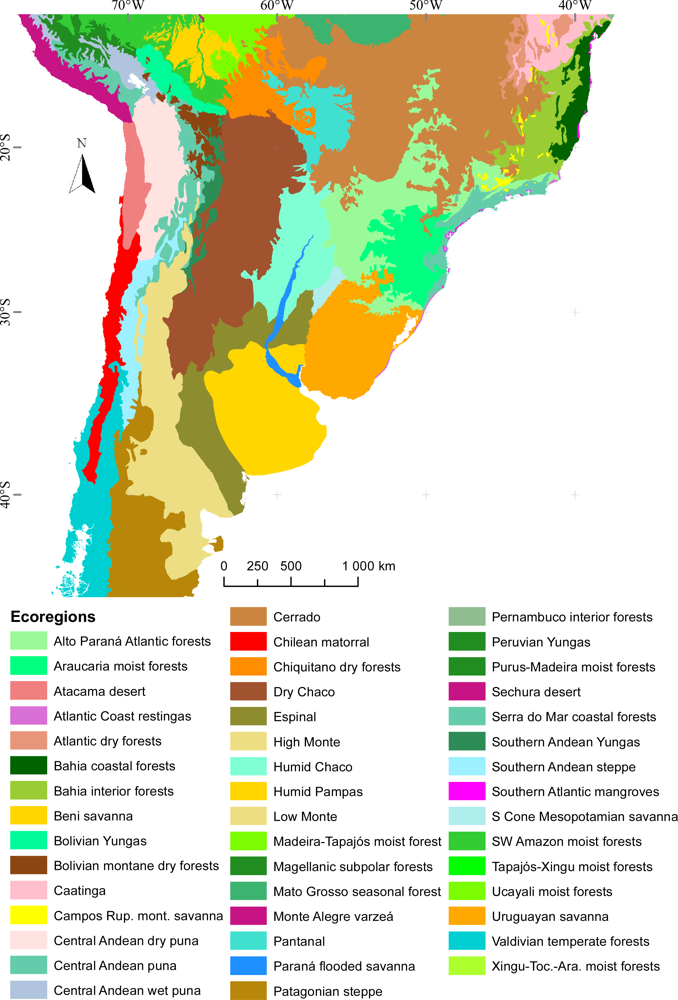
Figure 2.
Ecosystem Functional Types (EFT) of temperate South America based on Moderate Resolution Imaging Spectroradiometer Enhanced Vegetation Index (MODIS-EVI) dynamics (0.05° pixel). The map shows the EFTs corresponding to the median of the 2001–2008 period. Capital letters correspond to the EVI annual mean (EVI_Mean) level, ranging from A to D for low to high productivity. Small letters show the seasonal coefficient of variation (EVI_sCV), ranging from a to d for high to low seasonality of carbon gains. The numbers indicate the season of maximum EVI (DMAX): (1) spring, (2) summer, (3) autumn, (4) winter. The map uses the 0.05º Global Climate Model Grid in geographic projection.
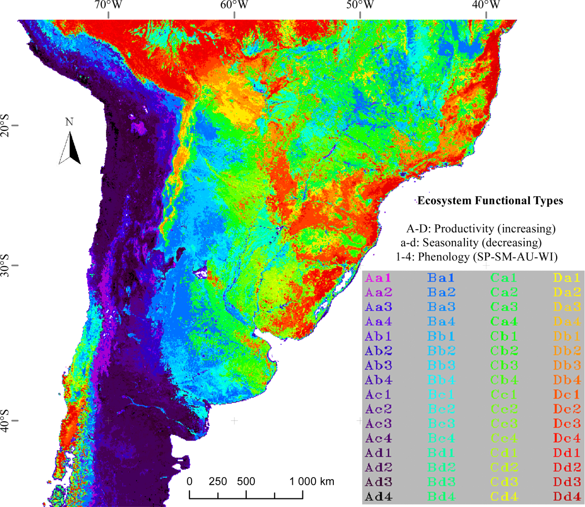
Figure 3.
Mean EFT richness across the different ecoregions of South America. Error bars indicate the spatial standard deviation.
Figure 3.
Mean EFT richness across the different ecoregions of South America. Error bars indicate the spatial standard deviation.

Figure 4.
Spatial patterns of Ecosystem Functional Types richness in temperate South America. The map shows the number of EFTs in each 0.05° × 0.05° grid cell. Rivers and water bodies are shown in white and ecoregion borders in gray.
Figure 4.
Spatial patterns of Ecosystem Functional Types richness in temperate South America. The map shows the number of EFTs in each 0.05° × 0.05° grid cell. Rivers and water bodies are shown in white and ecoregion borders in gray.
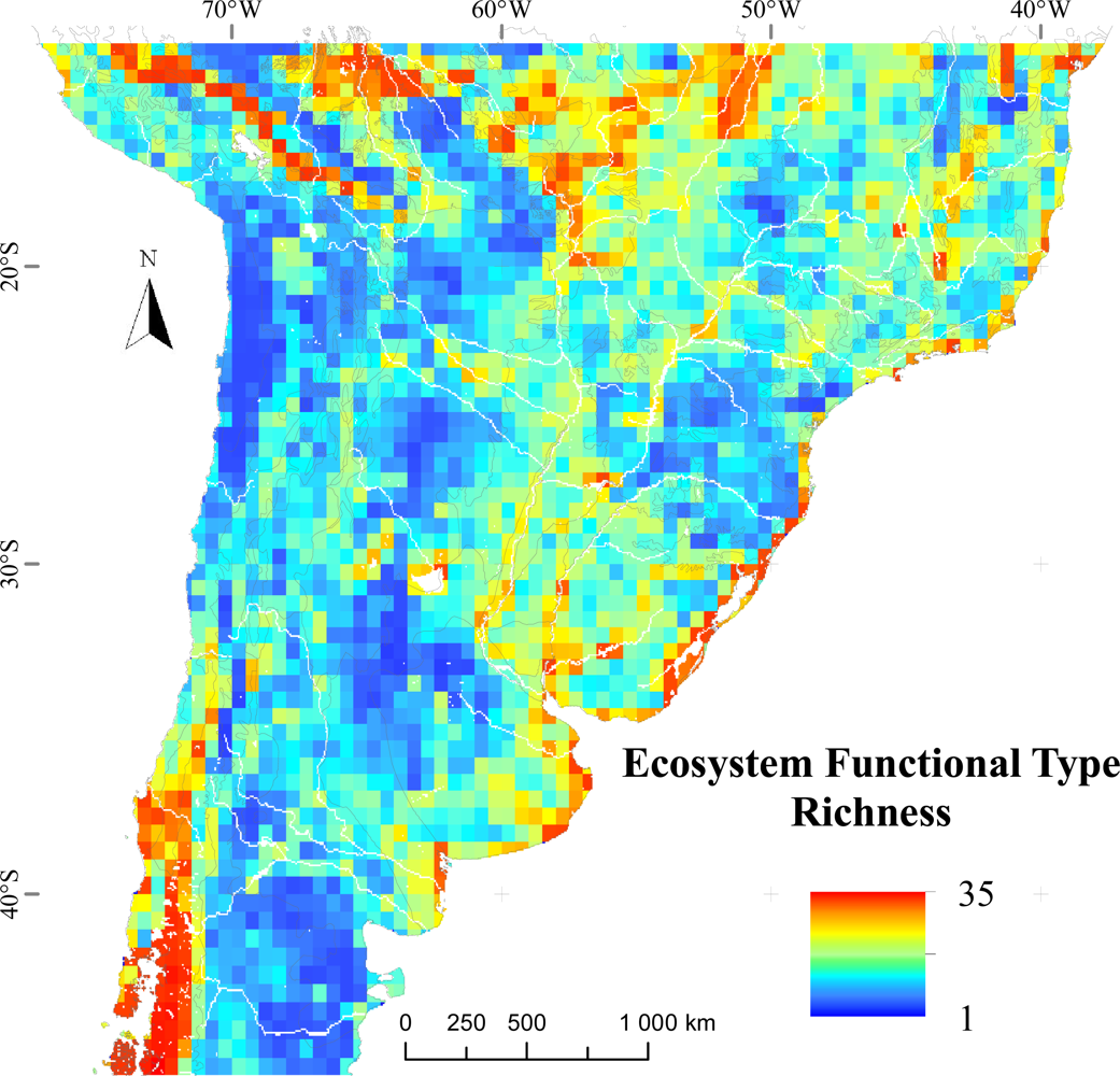
Figure 5.
Relationship between EFT richness and “water availability” variables. The sense of the effect was visualized by using warmer colors for high point density and Local Polynomial Regression Fitting (LOESS) on the 10th, 50th and 90th percentile. Relationships were compared across a Human Influence Index (HII) gradient: natural (HII < 10), mixed (10 < HII < 20) and anthropogenic systems (HII > 20). PctWatBodies: % of water bodies; Dist2Wat: distance to water; Pre: precipitation; WetDaysFrq: wet days frequency.

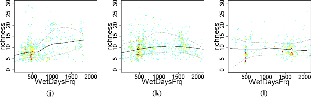
Figure 6.
Relationship between the EFT richness and “energy - water availability” variables. To visualize the sense of the effect, we used warmer colors for high point density and Local Polynomial Regression Fitting (LOESS) on the 10th, 50th and 90th percentile. Relationships were compared across a Human Influence Index (HII) gradient: natural ecosystems (HII < 10), mixed (10 < HII < 20) and anthropogenic systems (HII > 20). PET: potential evapotranspiration; sCV_PET: seasonal coefficient of variation of potential evapotranspiration; sCV_VapP: seasonal coefficient of variation of vapor pressure.
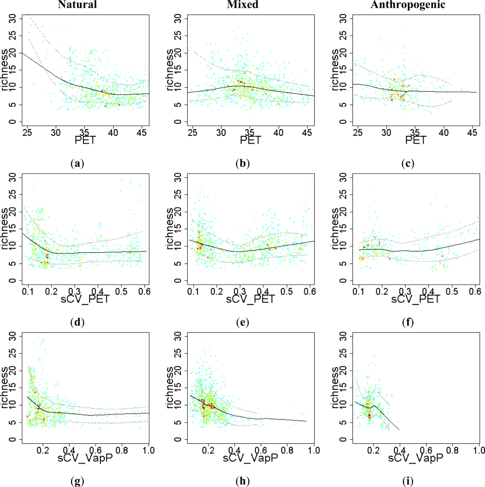
Figure 7.
Relationship between the EFT richness and “energy” and “relief” variables. To visualize the sense of the effect, we used warmer colors for high point density and Local Polynomial Regression Fitting (LOESS) on the 10th, 50th and 90th percentiles. Relationships were compared across a Human Influence Index (HII) gradient: natural (HII < 10), mixed (10 < HII < 20) and anthropogenic systems (HII > 20). Tmp: temperature; DTR: diurnal temperature range; sCV_DTR: seasonal coefficient of variation of DTR.


Figure 8.
Relationship between the EFT richness and “human influence” variables. To visualize the sense of the effect, we used warmer colors for high point density and Local Polynomial Regression Fitting (LOESS) on the 10th, 50th and 90th percentiles. Relationships were compared across a gradient of Human Influence Index (HII): Natural ecosystems (HII < 10), mixed (10 < HII < 20) and anthropogenic systems (HII > 20). CV: spatial coefficient of variation; Pct: percentage.


Table 1.
Deviance explained by the different Poisson Generalized Linear Models fitted between EFT richness and each explanatory variable (x1 column) or its quadratic transformation (x2 column). Models were compared across a gradient of the Human Influence Index (HII): Natural ecosystems (0 < HII < 10), mixed (10 < HII < 20) and anthropogenic systems (20 < HII < 40). Deviances are shown where p-values for the ANOVA Chi2 tests are lower than 0.01. The color scale is used to visualize, in green, those models that cumulated the greatest explained deviances and, in red, the lowest within the same category of human influence.
| Explained Deviance | Natural.x1 | Natural.x2 | Mix.x1 | Mix.x2 | Anthropogenic.x1 | Anthropogenic.x2 | |
|---|---|---|---|---|---|---|---|
| Water | %Water Bodies | 0.09 | 0.11 | 0.06 | 0.06 | 0.13 | 0.13 |
| Dist2Wat | 0.15 | 0.17 | 0.01 | 0.03 | 0.04 | 0.06 | |
| Precipitation | 0.14 | 0.24 | 0.03 | 0.10 | |||
| WetDaysFrq | 0.15 | 0.16 | 0.01 | 0.06 | |||
| sCV_Pre | 0.09 | 0.09 | 0.05 | ||||
| Water - Energy | PET | 0.19 | 0.22 | 0.05 | 0.05 | 0.03 | 0.03 |
| sCV_PET | 0.01 | 0.10 | 0.12 | 0.05 | |||
| sCV_VapP | 0.07 | 0.12 | 0.11 | 0.11 | 0.05 | 0.06 | |
| Energy | Temperature | 0.03 | 0.08 | 0.02 | |||
| DTR | 0.13 | 0.13 | 0.01 | 0.04 | 0.04 | 0.05 | |
| sCV_Tmp | 0.01 | 0.02 | 0.01 | 0.03 | |||
| sCV_DTR | 0.09 | 0.12 | 0.04 | 0.05 | |||
| sCV_FrostFrq | 0.02 | 0.02 | 0.03 | 0.03 | |||
| Relief | CV_Altitude | 0.02 | 0.02 | 0.06 | 0.06 | 0.18 | 0.20 |
| Human influence | %Croplands | 0.02 | 0.02 | 0.15 | 0.15 | ||
| %Pastures | 0.06 | 0.07 | 0.01 | 0.03 | 0.04 | 0.07 | |
| HII | 0.01 | ||||||
| CV_%Cropland | 0.07 | 0.07 | 0.02 | 0.06 | 0.16 | ||
| CV_%Pastures | 0.05 | 0.05 | 0.01 | ||||
| CV_HII | 0.01 | 0.01 | 0.14 | 0.15 | |||
Dist2Wat: distance to water bodies, WetDaysFrq: wet days frequency, sCV_Pre: seasonal coefficient of variation of precipitation, PET: potential evapotranspiration, sCV_VapP: seasonal coefficient of variation of vapor pressure, DTR: diurnal temperature range, sCV_Tmp: seasonal coefficient of variation of temperature, sCV_DTR: seasonal coefficient of variation of diurnal temperature range, sCV_FrostFrq: seasonal coefficient of variation of frost frequency, CV_Altitude: spatial coefficient of variation of altitude, HII: human influence index.
Table 2.
Akaike Information Criteria of the different Poisson Generalized Linear Models fitted between EFT richness and each explanatory variable (x1 column) or its quadratic transformation (x2 column). Models were compared across a gradient of the Human Influence Index (HII): Natural ecosystems (0 < HII < 10), mixed (10 < HII < 20) and anthropogenic systems (20 < HII < 40). The color scale is used to visualize, in green, those models that showed the lowest AIC values and, in red, the greatest within the same category of human influence.
| AIC | Natural.x1 | Natural.x2 | Mix.x1 | Mix.x2 | Anthropogenic.x1 | Anthropogenic.x2 | |
|---|---|---|---|---|---|---|---|
| Water | %Water Bodies | 5182 | 5151 | 6132 | 6127 | 2460 | 2462 |
| Dist2Wat | 5083 | 5046 | 6201 | 6172 | 2515 | 2507 | |
| Precipitation | 5086 | 4908 | 6176 | 6074 | 2537 | 2531 | |
| WetDaysFrq | 5076 | 5053 | 6207 | 6129 | 2536 | 2537 | |
| sCV_Pre | 5192 | 5191 | 6218 | 6146 | 2538 | 2538 | |
| Water - Energy | PET | 5011 | 4943 | 6144 | 6141 | 2522 | 2522 |
| sCV_PET | 5331 | 5174 | 6221 | 6045 | 2530 | 2512 | |
| sCV_VapP | 5217 | 5125 | 6049 | 6049 | 2506 | 2504 | |
| Energy | Temperature | 5286 | 5199 | 6213 | 6200 | 2536 | 2533 |
| DTR | 5120 | 5114 | 6206 | 6162 | 2514 | 2513 | |
| sCV_Tmp | 5335 | 5305 | 6200 | 6186 | 2538 | 2539 | |
| sCV_DTR | 5186 | 5128 | 6154 | 6150 | 2534 | 2534 | |
| sCV_FrostFrq | 5314 | 5306 | 6223 | 6222 | 2522 | 2524 | |
| Relief | CV_Altitude | 5315 | 5312 | 6129 | 6130 | 2428 | 2423 |
| Human influence | %Croplands | 5346 | 5348 | 6195 | 6193 | 2452 | 2450 |
| %Pastures | 5234 | 5230 | 6206 | 6177 | 2517 | 2500 | |
| HII | 5346 | 5331 | 6223 | 6216 | 2537 | 2532 | |
| CV_%Cropland | 5214 | 5214 | 6213 | 6194 | 2503 | 2445 | |
| CV_%Pastures | 5264 | 5261 | 6211 | 6212 | 2538 | 2540 | |
| CV_HII | 5331 | 5324 | 6221 | 6223 | 2456 | 2449 |
Dist2Wat: distance to water bodies, WetDaysFrq: wet days frequency, sCV_Pre: seasonal coefficient of variation of precipitation, PET: potential evapotranspiration, sCV_VapP: seasonal coefficient of variation of vapor pressure, DTR: diurnal temperature range, sCV_Tmp: seasonal coefficient of variation of temperature, sCV_DTR: seasonal coefficient of variation of diurnal temperature range, sCV_FrostFrq: seasonal coefficient of variation of frost frequency, CV_Altitude: spatial coefficient of variation of altitude, HII: human influence index.
Share and Cite
MDPI and ACS Style
Alcaraz-Segura, D.; Paruelo, J.M.; Epstein, H.E.; Cabello, J. Environmental and Human Controls of Ecosystem Functional Diversity in Temperate South America. Remote Sens. 2013, 5, 127-154. https://doi.org/10.3390/rs5010127
AMA Style
Alcaraz-Segura D, Paruelo JM, Epstein HE, Cabello J. Environmental and Human Controls of Ecosystem Functional Diversity in Temperate South America. Remote Sensing. 2013; 5(1):127-154. https://doi.org/10.3390/rs5010127
Chicago/Turabian StyleAlcaraz-Segura, Domingo, José M. Paruelo, Howard E. Epstein, and Javier Cabello. 2013. "Environmental and Human Controls of Ecosystem Functional Diversity in Temperate South America" Remote Sensing 5, no. 1: 127-154. https://doi.org/10.3390/rs5010127