Snow Grain-Size Estimation Using Hyperion Imagery in a Typical Area of the Heihe River Basin, China

1
School of Geographic & Oceanographic Sciences, Nanjing University, Nanjing 210093, China
2
Jinan Environmental Monitoring Center Station, Jinan 250014, China
*
Author to whom correspondence should be addressed.
Remote Sens. 2013, 5(1), 238-253; https://doi.org/10.3390/rs5010238
Submission received: 11 November 2012
/
Revised: 31 December 2012
/
Accepted: 4 January 2013
/
Published: 11 January 2013
Abstract
:It is difficult and time consuming to use traditional measurement methods to estimate the physical properties of snow. However, the emergence of hyperspectral imagery for estimating the physical properties of snow provides a powerful tool. Snow albedo, grain size, and temperature are important factors for evaluating the surface energy balance. Using the spectrum-reflection curves of the different grain sizes of snow measured in the fields of the Binggou watershed of the Heihe River Basin, China, we analyzed the spectral reflection characteristics of snow. A statistical detection method was used to choose the most sensitive bands in the field spectra and find the corresponding band (band 89) in the Hyperion imagery. The bands near 1033 nm were sensitive to the snow grain size. According to the relationship between the snow grain size and the measured spectrum, we built a snow grain-size estimation model. The results showed that the snow reflectance had a good linear and exponential relationship with the snow grain size. The correlation coefficients R of the two models were 0.81 and 0.84, respectively. We obtained the location of the absorption valley at the near-infrared wavelength, and the results showed that 6.9% of the pixels were affected by the snow water content. The locations of the absorption valley moved 1–4 bands from band 89 to shorter wavelengths. The accuracy of the snow grain size estimates based on the Hyperion imagery was relatively high.
1. Introduction
Snow is an important subject of cryosphere-environment science and is a useful environmental indicator of global changes in terms of long-term monitoring [1]. The temporal and spatial distribution of snow cover is an important indicator of the climate [2]. As one of the optical characteristics of snow, snow grain size is an important factor causing albedo changes and thus is also one of the factors affecting the global radiation balance.
Assuming snow grains to be granular spheres and ignoring the scattering effect between grains in the “near-field,” the “delta-Eddington” approximation for multiple scattering together with Mie theory for single scattering could be used to calculate the scattering of individual snow grains. Wiscombe and Warren found effects of grain size on reflectance spectra [3]. The researchers noted that (1) when the snow grain size becomes larger, the absorption and forward scattering of snow increases, and (2) the snow surface reflectance declines with increasing grain size, and, as the grain size grows, the absorption intensity in near-infrared bands is larger than in the visible bands. Dozier et al. used the theoretical model of Wiscombe and Warren and NOAA-6 AVHRR data to highlight that using remote sensing tools to measure the snow grain size was a potentially effective method [4], but their result was difficult to interpret because the authors did not address near-infrared bands, which were sensitive to grain size in the NOAA-6 AVHRR data.
According to Landsat TM images, snow types have been classified as: clean new snow, older metamorphosed snow, and snow mixed with vegetation [5], but the results were not verified with measured data at the time of the satellite transit. The contaminant content of the snow mainly affected the reflectivity in the visible range; however, the near-infrared reflectance depended on the snow grain size. The estimated results based on the TM band 4 in the near-infrared range were close to the measured data, although no atmospheric correction of the Landsat TM images was completed [6].
Nolin and Dozier used an airborne visible/infrared imaging spectrometer (AVIRIS) and discrete-ordinate model to calculate directional reflectance as a function of snow grain size [7]. Their inversion method was validated using measured data and had a higher accuracy for solar incidence angles between 0° and 30°. The authors improved their model by using a radiative transfer model based on the near-infrared reflectance characteristics of snow to obtain a quantitative retrieval of snow grain size [8]. This method had a higher accuracy and fewer errors caused by topography.
Hemisphere-directed reflections of snow cover at the wavelengths of 1.8 μm and 2.2 μm have been used to estimate snow grain size based on MODIS/ASTER data [9]. However, this approach caused large errors when the grain size was large, and the method was greatly impacted by the atmosphere and solar radiation. The normalized index or relative reflectivity of the MODIS band may estimate the snow grain size more accurately and robustly [10–12].
Several snow grain size inversion models and algorithms have been established, including models based on optical scattering theory, single-channel inversion algorithms, and ratios of multichannel algorithms. Previous images for inversion are, generally, multispectral images with low or medium spatial resolution, e.g., AVHRR or MODIS, and high resolution multispectral images, such as Landsat TM, or airborne hyperspectral images, such as AVIRIS. However, the number of studies estimating snow grain size using hyperspectral aerospace images is limited, especially combining both synchronized hyperspectral spectrometer data and snow grain size data. In this study, we used the Earth Observing-1 (EO-1) Hyperion hyperspectral imagery, which also has a high resolution, to establish the relationship between the bands and the snow grain size based on the spectral analysis of ground-synchronized measurement data. The study aimed to estimate the snow grain-size distribution of the Heihe River Basin region in the Binggou watershed and evaluate the estimates using ground-measured data.
2. Materials and Methodology
2.1. Study Area and Data
The study area is located in a typical region of the Heihe River Basin in the Binggou watershed of the Qilian Mountains. The Binggou watershed (38°01′N–38°04′N, 100°12′E–100°18′E) is located in one level 2 branch of the Qilian Mountains, upstream of the Heihe River Basin. The average elevation of the area is 3,920 m. The watershed area is 30.48 square kilometers and belongs to the permafrost regions of the western high mountain plateau. This area has abundant precipitation, and the average annual rainfall is 774 mm. The region has a continental climate, and the snow is seasonal. Interaction of the terrain and high-speed wind results in large-scale redistributions of snow. The annual average, minimum, and maximum temperatures are −2.5°C, −30.8°C, and 24.8°C, respectively. The average snow depth is approximately 0.5 m, and the greatest depths can reach 0.8–1.0 m. In the study, we selected eight flat sample plots: A, B, C, D, E, F, G and H. The A and B plots were 270 × 270 m2 in size, the C, F, G and H plots were 120 × 120 m2 in size, and the D and E plots were 90 × 90 m2 in size. Figure 1 shows the plot locations.
2.2. Data Collection and Pre-Processing of Hyperion Imagery
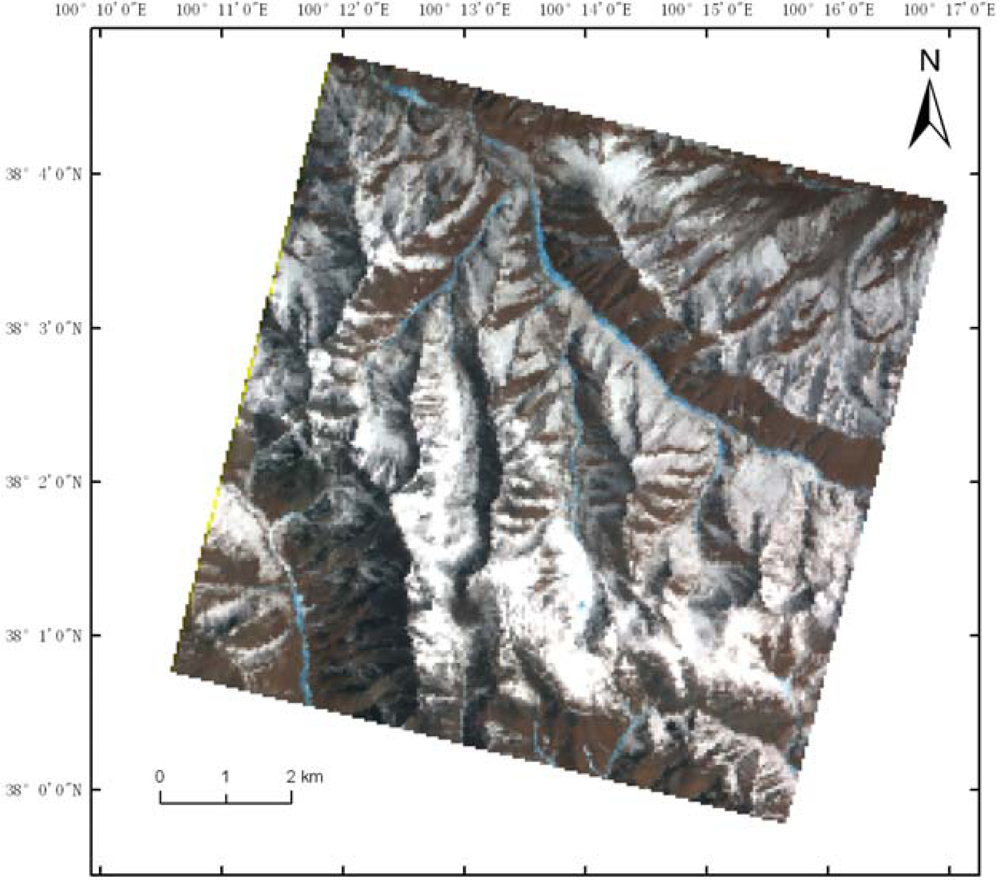
The present study used L1 production of EO-1 Hyperion imagery of the Binggou watershed of the upper Heihe River basin. The data were acquired at 11:47:50 a.m. on 17 March 2008. The zenith and azimuth angles of the sun at the time of the data collection were 45.5° and 143.85°, respectively. The sensor delivered 242 spectral channels, and the spatial resolution was 30 m. The Hyperion imagery of the study area is plotted in Figure 2.
In this study, the pre-processing included five steps. They are removal of non-calibrated bands and bands that affected by water vapor, geometric correction, absolute radiation of the values of the conversion, brightness-stripe removal, and atmospheric correction. Here we used the 6S (Second Simulation of the Satellite Signal in the Solar Spectrum) model to conduct the atmospheric correction of the Hyperion bands 81–94.
2.3. Spectrum Observation and Measurements of Snow Grain Size
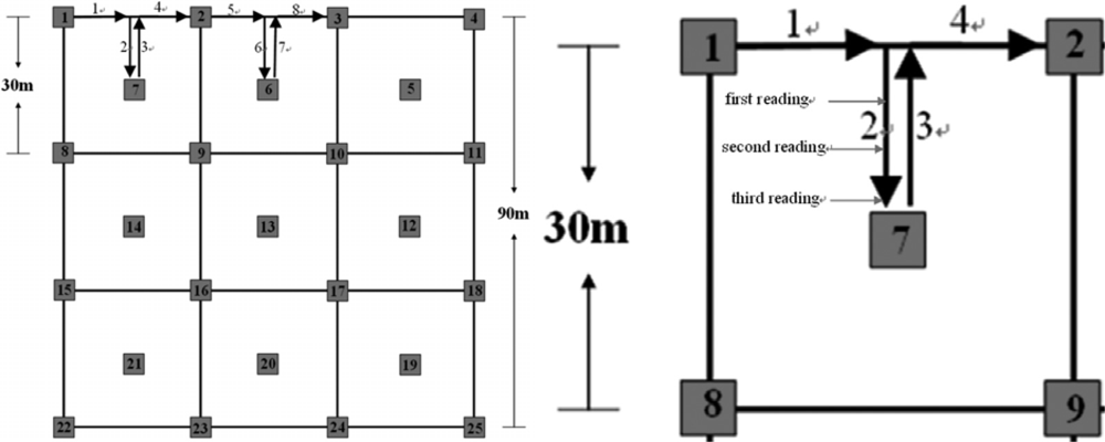
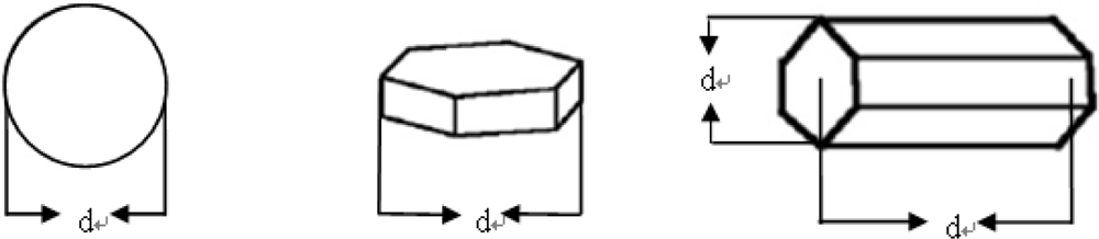
Snow spectra measurements were obtained using a single-channel field-portable radiation spectrometer from the American ASD company. The spectrum experiments were conducted in the eight flat sample plots (A, B, C, D, E, F, G and H) between 9:00 am and 12:00 am from 14 March to 22 March 2008. Each 30 m × 30 m plot corresponded to a Hyperion image pixel. We obtained approximately 244 pairs of grain size and spectral data under ideal conditions per day. The experiments ensured a sufficient solar-elevation angle and that the data were synchronous with the EO-1 Hyperion remote-sensing satellite. Typically, the spectral data were collected under the following conditions: (a) the ground visibility exceeded 10 km, (b) the cloud cover was less than 2% within the solar solid angle of 90°, and (c) the wind velocity was lower than 5.4 m/s. The data that complied with these conditions were chosen for analysis. On the satellite transit day (17 March 2008), we obtained 233 pairs of valid data and selected 70 pairs of the data randomly to establish an estimation model and the remaining 163 pairs to validate the model. In the measurements of the snow spectral reflectance, simultaneous observations of snow particle size were conducted using a portable handheld microscope, which magnifies 40 times. We complied with the following demands of the measurement process: (a) the destruction of the snow surface must be avoided as much as possible (Figure 3), (b) measurements must be conducted 3 times in every 30 m × 30 m plot, (c) the snow cover must be treated in layers of 10 cm and the snow grain size read in the surface and in the middle of every depth layer, (d) the staff must be dressed in dark clothing with their backs to the sun and conduct the measurements in the shadows, and (e) the size must be estimated according to the shape of the snow particles, the average position of a particle’s major and minor axes relative to the center column, and the diameter of the sphere and plate (Figure 4).
2.4. Analysis of the Measured Spectral Data
The ratio of snow to whiteboard-radiation brightness can be evaluated as the snow reflectance. Figure 5 shows the snow spectral reflectance sampled in the Binggou watershed. The snow reflectivity in the visible light region was relatively high, normally between 0.6 and 0.95 (Figure 5). The value decreased rapidly in the near-infrared region. Four absorption valleys appeared near 1,030 nm, 1,250 nm, 1,470 nm, and 2,000 nm. However, the value of reflectivity was almost zero near 1,470 nm and 2,000 nm, and the types of snow showed very small differences between these two wavelengths. Thus, to find the band that is sensitive to snow-particle size, one should focus on the near-infrared region, of which the corresponding bands in the Hyperion hyperspectral imagery could not be easily affected by water vapor, atmospheric scattering or attenuation.
The experiments were conducted between 9:00 am and 12:00 am, with a solar-elevation angle typically greater than 30°. With an increase of the solar elevation angle, the reflectivity of the snow surface decreased. To analyze the relationship between the spectral curves and snow-particle size near the near-infrared region, it was necessary to introduce amendments to the solar elevation angle [13]. To simplify the calculations, this research assumed a linear relationship of the snow reflectivity corresponding to the solar elevation angles at one wavelength.
Different wavelengths had different penetration depths through the snow layer, even with the same particle size. At the same wavelength, the penetration depths differed for different particle sizes. Stamnes et al. defined the photon-penetration depth as the radiation flux-attenuation depth [14], as follows:
where a is the penetration depth, h is the thickness of the snow layers, F is the downward radiation flux at h, and Fs is the downward radiation flux at the snow surface. For the wavelengths near 1,030 nm, the penetration depth of a snow layer was normally within 10 cm. Therefore, this research used the average particle size of the surface and the 0–10 cm depth snow layer to establish the relationships between the spectral curves and snow particle sizes.
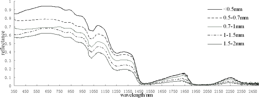
According to the different particle sizes in each pixel, the particle sizes were divided into five categories: <0.5 mm, 0.5–0.7 mm, 0.7–1 mm, 1–1.5 mm, and 1.5–2 mm. Twenty spectral curves of each category were chosen, and the means were calculated to obtain the snow spectral curves, as shown in Figure 6.
It can be seen from Figure 6 that the snow of different particle sizes had various spectral curves. In general, the snow with larger particle sizes had lower values of reflectivity. Whether in the visible or near-infrared region, the spectral curves of the different particle sizes obviously varied. However, a very small amount of strongly absorbent particles in the snow would decrease the snow reflectivity by 5%–15% in the visible region. In contrast, these particles barely had any effect on the snow reflectance when the wavelength was greater than 900 nm [15]. Therefore, to avoid this situation, we must select a band in the near-infrared region.
2.5. The Optimal Band Selection to Estimate Grain Size
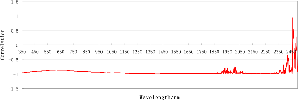
To discuss the quantitative relationship between the snow grain size and spectral reflectance, we selected 20 spectrum curves of each of the different snow types and analyzed the spectral reflection and grain size for each type to identify the correlations between them. Figure 7 shows the correlation coefficients between the grain size and the light spectrum.
Figure 7 indicates that generally, the snow reflectivity and grain size are negatively correlated. A greater grain size corresponds to a lower snow reflectivity. From the absolute value of the related coefficient, we can see there is a good correlation between the snow reflectivity and grain size in the wavelength range between 950 and 1,750 nm. Combined with Figure 6, it can be seen that a wavelength greater than 1,150 nm will lead to a low reflectivity and is not beneficial to estimate snow parameters.
Reflectivity generally varies continuously as a function of grain size. We used the variogram to find what wavelength is most appropriate for determining grain size. We calculated the M, the total of variogram for different grain sizes in the wavelength range of 700 nm to 1,300 nm. A band with a larger M is a better choice. The following formula was used to calculate the M :
where Z is the snow reflectances of the grain sizes, Xi is snow grain sizes, Δh is 0.1 mm, which is the reading accuracy of the portable handheld microscope, n is the number of categories of grain sizes.
The distribution of the M value along the wavelength bands is illustrated in Figure 8.
Figure 8 shows an apparent peak of the M function at the wavelength near 1,030 nm. The band near 1,030 nm was an obvious absorption valley of the snow reflection in the near-infrared region of the spectrum, and this band was less affected by atmospheric scattering and attenuation; therefore, we chose this band as the study object.
2.6. Extraction of Snow Cover and Histogram Statistics
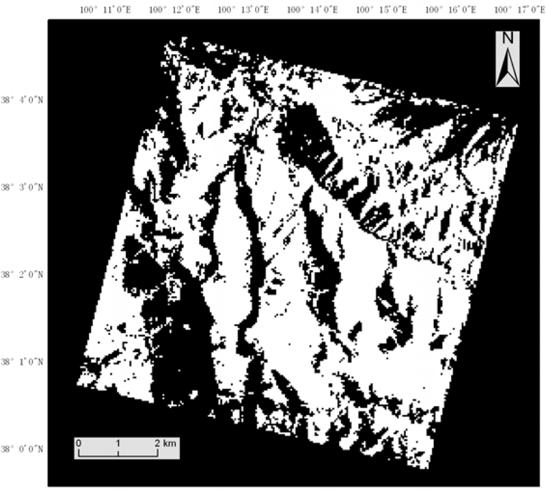
Before we estimated the grain size, we had to extract the snow cover, which requires the separation of the snow-covered surface and non-snow-covered surface. Currently, there are five main methods to extract snow cover using remote-sensing data. They are visual interpretation, a multiband imagery calculation, the brightness-threshold method, a snow-cover index, and a radiative transfer model. Considering the characteristics of the Hyperion imagery and noting that there were no clouds in the sky, we combined a brightness threshold and snow-cover indexing method to extract snow cover in this study, as presented in the following equation:
Figure 9 shows the distribution of the extracted snow cover. There were 39,301 snow pixels in the whole Binggou watershed image, with a snow-covered area of 3.53 million square meters, accounting for 61% of the Binggou watershed image.
2.7. Band Histogram Statistics
The 1,030 nm wavelength in the hyperspectral images corresponded to the Hyperion band 89 (1,033.5 nm). The mathematical statistics of the Hyperion imagery after atmosphere correction showed that the maximum value was 0.825 and that the average value was 0.346. The standard deviation was 0.135. Figure 10 contains the image histogram statistics.
3. Results and Discussion
3.1. Expression of the Grain-Size Estimation Model
Figure 11 indicates the relationship between the pixel value of the Hyperion band 89 after atmospheric correction and the snow grain size. Linear fitting and curve fitting of the pixel value and grain size led to the following relationships, respectively: ρ = −0.26R + 0.67, where ρ is the reflectance, R is the snow grain size. The correlation coefficient r of the fitting line was 0.81. ρ = 0.47R−0.51, the correlation coefficient r was 0.84. The root mean square error (RMSE) was 0.24 mm and 0.21 mm for the linear fitting and curve fitting, respectively. These results indicate that the pixel value had an index function and a linear relation with the grain size.
3.2. Mapping the Snow Grain Size Using the Hyperion Imagery
According to the linear and exponential models, we classified the snow into five categories based on the grain size, as shown in Figure 12.
Figure 12 indicates that the estimation results of the snow grain size using the linear model and exponential model were almost the same. A total of 11.7% of the snow had a grain size less than 0.5 mm; 16.2% was between 0.5 mm and 0.7 mm; 20.7% was between 0.7 mm and 1 mm; 26.2% was between 1 mm and 1.5 mm; and, 25.5% was between 1.5 mm and 2 mm. Similar estimates resulted due to the similar function curves of the two models in the grain-size range of 0.5–1.5 mm. There were differences only in the grain-size ranges of less than 0.5 mm and greater than 1.5 mm.
3.3. Improvement of the Snow Grain-Size Estimation Model
In this study, we selected a dry snowy surface as test plot to facilitate the reading of the snow grain size. However, the water content of the Binggou watershed is inconsistent, and water has a strong absorption band in the near-infrared bands near 980 nm. Because the contaminant content of the snow mainly affected the reflectivity in the visible range and almost no effect on snow albedo beyond 900 nm wavelength [15], the snow’s water content maybe the main reason of causing the spectrum-absorption valley in the near-infrared bands to shift in a short-wave direction.
For the Hyperion imagery, the snow absorption valley of the near-infrared bands was not necessarily in band 89, which led to a high snow reflectance error of a single band. In the study, we explored the location of snow spectrum-absorption valleys in the near-infrared bands. There were 36,747 pixels in the normal absorption position, which is band 89. There were 2,329 pixels whose absorption-valley location moved to band 88, 110 pixels moved to band 87, 108 pixels moved to band 86, and 7 pixels moved to band 85, as shown in Figure 13.
We assumed that the snow’s water content was proportional to the movement of the spectrum absorption valley and that the location reflected the water content of the snow. Using models of the snow reflectance and snow grain size in band 89 will result in large errors. For the 2,554 pixels that had spectrum absorption-valley movement, we could replace the assumed snow-reflectance wavelength with the new one. Figure 14 shows the new distribution of the snow grain size. These abnormal pixels were affected by both the snow humidity and grain size. The relationship between the reflectance and snow characteristics was not a simple linear or exponential relationship, and there were no measured data. The estimation accuracy of the method requires further study.
3.4. Assessment of Snow Grain-Size Estimation Results
It can be seen from the distribution of the snow grain-size inversion that the snow grain size is relatively small in places with less sunlight, such as valleys and shady slopes, and vice versa, which is consistent with the actual situation. Snow in valleys and on shady slopes can easily maintain the characteristics of new snow. Snow on sunny slopes is often affected by sunlight and wind, which lead to significant deterioration.
Remote-sensing inversion data can be validated using directly measured snow grain sizes [6,12,16,17]. The remaining 163 measured snow grain-size data in Section 2.3, corresponding to 163 pixels of the Hyperion imagery, were synchronized with the transit time of the hyperspectral remote-sensing satellite. The RMSE were calculated for both the linear and exponential models as follows:
where yi is the measured value, ŷ is an estimated value, and n is the number of samples. The RMSE were 0.14 mm and 0.12 mm for the linear model and the exponential model, respectively. The linear relationship between the estimated and measured snow grain sizes was calculated and shown in Figure 15. The linear relationship coefficient r2 is 0.86. The kappa coefficient of the estimate accuracy was calculated (Table 1).
3.6. Uncertainties
First, the error of the measured spectral data could be caused during the field measurement. The standard reference versions of the spectral resolution, central wavelength position, signal-to-noise ratio, and diffuse reflectance are less precise. The staff and the surrounding environment will also have an impact the measured spectra. The low signal-to-noise ratio of the SWIR bands is lower than that of the VNIR bands for the Hyperion data. The low signal-to-noise ratio of the Hyperion data may impact the estimation accuracy. This problem may be addressed by using multiple bands near 1,030 nm, which can average one single-band noise.
The change in snow reflectance caused by the sun’s elevation angle is not a simple linear relationship, and the changes caused by different wavelengths of snow reflectance with solar elevation angle are also different. We cannot obtain reflectance data with the same snow-surface conditions but with different solar elevation angles, and therefore, it is difficult to correct for the solar altitude angle. The analysis results can also be affected.
Secondly, measurement error of snow grain size. Currently, the best measurement method of grain size is to extract a snow sample for observation using three-dimensional measurement techniques at a low-temperature laboratory [4,18,19]. This technology can be used to observe not only the snow grain size but also the snow volume and surface area. However, with limited conditions, we used a hand-held 40-times-magnified calibrated microscope to measure the grain size and record the long axis diameter and shape of the snow particles. Measurements of the spectrum and grain size cannot be fully synchronized in exactly the same environment, which means that there will be subtle changes in the measurement process. Operating personnel may introduce reading errors due to different snow particle shapes. Different particle shapes also affect the optical properties of snow [20,21]. Forward-reflected radiances and backscattering radiances may be overestimated or underestimated, regardless of the particle shapes.
The topography can affect the snow reflectance, especially if there is shaded area. The normalized reflectance, like the absorption band depth or area [8], may reduce the topographic effect to a certain extent. Considering that the topography of the study area was mainly aligned from north to south and the satellite-transit time was close to noon, we used a single-band model. In further work, we may combine the images with DEM data to remove the topography influence.
Different wavelengths have different snow penetration depths, and a single wavelength also has different penetration depths with different grain sizes. The penetration depth of a snow layer was normally within 10 cm near the wavelength of 1,030 nm. The estimated results only represent the snow grain size within 10 cm depth. The estimation of the grain size at different depths is a problem worth further exploration.
4. Conclusions
The wavelength near 1,030 nm is most sensitive to snow grain size, which was found by implementing the variogram algorithm based on the analysis of field spectral and snow grain size measurements in the paper. This wavelength corresponding to band 89 of Hyperion imagery, whereby the waveband center is 1,033.5 nm and band width is 10 nm. We built linear and exponential models using band 89 to estimate snow grain size in the Heihe River Basin, China, and found that the exponential relationship performed slightly better than the linear correlation. The square of the correlation coefficient between estimated and measured snow grain sizes is 0.86 and the Kappa coefficient of the estimate accuracy is 0.611.
Furthermore, water had a strong absorption band in the near-infrared region at approximately 980 nm (band 63 on Hyperion imagery). Thus, the water content in snow may cause the near-infrared snow-spectrum absorption to shift to shorter wavelengths. We calculated the location of the absorption and showed the influence of water content on some pixels, in which the wavelength of the absorption shifted 1–4 bands from band 89.
The current model can be run operationally and has a robust performance over the study area of the paper. However the model needs some further development. Therefore, future endeavors should focus on multibands and radar imaging to develop a method for estimating snow grain size at different depths, while considering the influence of the more irregular snow grain shapes.
Acknowledgments
This research work is supported by the National 973 Program (2010CB951503), a Western action plan project of the Chinese Academy of Science (KZCX2-XB2-09) and the Priority Academic Program Development of Jiangsu Higher Education Institutions. The authors thank Jian Wang from the Cold and Arid Regions Environmental and Engineering Research Institute, Chinese Academy of Sciences, and Xuezhi Feng and Pengfeng Xiao from the School of Geographic and Oceanographic Sciences, Nanjing University, for their help in the collection and observation of the snow data and Hyperion data. The authors also thank Guorong Hu of Geoscience Australia, Australia for modifying the paper. Finally, the authors thank the editor and the anonymous reviewers for their valuable advices.
References
- Rinne, J.; Aurela, M.; Manninen, T. A simple method to determine the timing of snow melt by remote sensing with application to the CO2 balances of northern mire and heath ecosystems. Remote Sens 2009, 1, 1097–1107. [Google Scholar]
- Kropacek, J.; Feng, C.; Alle, M.; Kang, S.; Hochschild, V. Temporal and spatial aspects of snow distribution in the Nam Co Basin on the Tibetan Plateau from MODIS data. Remote Sens 2010, 2, 2700–2712. [Google Scholar]
- Wiscombe, W.J.; Warren, S.G. A model for the spectral albedo of snow: I Pure snow. J. Atoms. Sci 1980, 37, 2712–2733. [Google Scholar]
- Dozier, J.; Davis, R.E.; Perla, R. On the Objective Analysis of Snow Microstructure. In Avalanche Formation, Movement and Effects; Salm, B., Gubler, H., Eds.; International Association of Hydrological Sciences Publication: Wallingford, UK, 1987; pp. 49–59. [Google Scholar]
- Dozier, J.; Marks, D. Snow mapping and classification from Landsat Thematic Mapper data. Ann. Glaciol 1987, 9, 97–103. [Google Scholar]
- Fily, M.; Bourdells, B.; Dedieu, J.P.; Sergent, C. Comparison of in situ and Landsat Thematic Mapper derived snow grain characteristics in the Alps. Remote Sens. Environ 1997, 59, 452–460. [Google Scholar]
- Nolin, A.; Dozier, J. Estimating snow grain size using AVIRIS data. Remote Sens. Environ 1993, 44, 231–238. [Google Scholar]
- Nolin, A.; Dozier, J. Hyperspectral method for remotely sensing the grain size of snow. Remote Sens. Environ 2000, 74, 207–216. [Google Scholar]
- Jennifer, E.K.; Alan, R.G.; Gary, B.H. Spatial relationships between snow contaminant content, grain size, and surface temperature from multispectral images of Mt. Rainier, Washington (USA). Remote Sens. Environ 2003, 86, 216–231. [Google Scholar]
- Scambos, T.A.; Haran, T.M.; Fahnestock, M.A. MODIS-based Mosaic of Antarctica (MOA) data sets: Continent-wide surface morphology and snow grain size. Remote Sens. Environ 2007, 111, 367–375. [Google Scholar]
- Lyapustin, A.; Tedesco, M.; Wang, Y.; Aoki, T.; Hori, M.; Kokhanovsky, A. Retrieval of snow grain size over greenland from MODIS. Remote Sens. Environ 2009, 113, 1976–1987. [Google Scholar]
- Painter, T.H.; Rittger, K.; McKenzie, C.; Slaughter, P.; Davis, R.E.; Dozie, J. Retrieval of subpixel snow covered area, grain size, and albedo from MODIS. Remote Sens. Environ 2009, 113, 868–879. [Google Scholar]
- Jiang, T.; Zhao, S.; Xiao, P.; Feng, X.; Zhang, Y.; Hu, W. Spectral analysis of different snow grain size based on field measurement. J. Glaci. Geoc 2009, 31, 227–232. [Google Scholar]
- Stamnes, K.; Li, W.; Eide, H.; Aoki, T.; Hori, M.; Storvold, R. ADEOS-II/GLI snow/ice products-Part I: Scientific basis. Remote Sens. Environ 2007, 111, 258–273. [Google Scholar]
- Warren, S.G.; Wiscombe, W.J. A model for the spectral albedo of snow. II: Snow containing atmospheric aerosols. J. Atoms. Sci 1980, 37, 2734–2745. [Google Scholar]
- Painter, T.H.; Molotch, N.P.; Cassidy, M.; Flanner, M.; Steffen, K. Contact spectroscopy for determination of stratigraphy of snow optical grain size. J. Glaciol 2007, 53, 121–127. [Google Scholar]
- Aoki, T.; Hori, M.; Motoyoshi, H.; Tanikawa, T.; Hachikubo, A.; Sugiura, K.; Yasunari, T.J.; Storvold, R.; Eide, H.A.; Stamnes, K.; et al. ADEOS-II/GLI snow/ice products Part II: Validation results using GLI and MODIS data. Remote Sens. Environ 2007, 111, 274–290. [Google Scholar]
- Grenfell, T.C.; Warren, S.G. Representation of a nonspherical ice particle by a collection of independent spheres for scattering and absorption of radiation. J. Geophys. Res 1999, 104, 31697–31709. [Google Scholar]
- Painter, T.H.; Dozier, J.; Roberts, D.A.; Davis, R.E.; Green, R.O. Retrieval of sub-pixel snow-covered area and grain size from imaging spectrometer data. Remote Sens. Environ 2003, 85, 64–77. [Google Scholar]
- Jin, Z.H.; Charlock, T.; Yang, P.; Xie, Y.; Miller, W. Snow optical properties for different particle shapes with application to snow grain size retrieval and MODIS/CERES radiance comparison over Antarctica. Remote Sens. Environ 2008, 112, 3563–3581. [Google Scholar]
- Picard, G.; Arnaud, L.; Domine, F.; Fily, M. Determining snow specific surface area from near-infrared reflectance measurements: Numerical study of the influence of grain shape. Cold Reg. Sci. Techol 2009, 56, 10–17. [Google Scholar]
Figure 1.
The distribution of the study plots in the Binggou watershed.
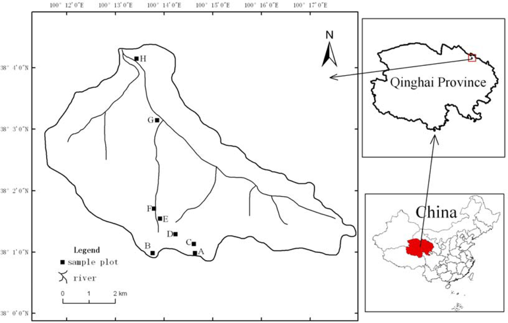
Figure 2.
EO-1 Hyperion imagery of the Binggou watershed area (R: band 96, G: band 34, B: band 19).

Figure 3.
The routes of measurement in the plots.

Figure 4.
The diameters of different snow-particle shapes.

Figure 5.
Snow spectral reflectance sampled in the Binggou watershed.
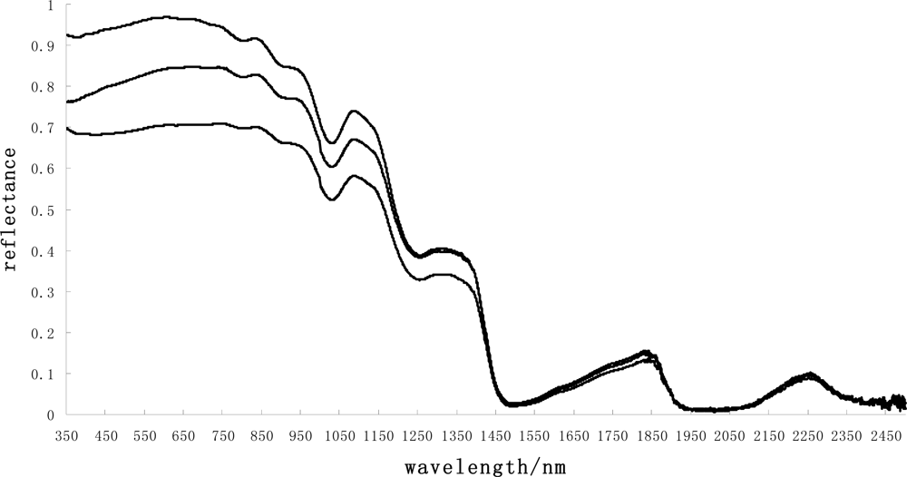
Figure 6.
Variation in the spectral reflectance at different snow grain sizes.

Figure 7.
The correlation coefficients between the grain size and light spectrum.

Figure 8.
The distribution of the M value along the wavelength bands.
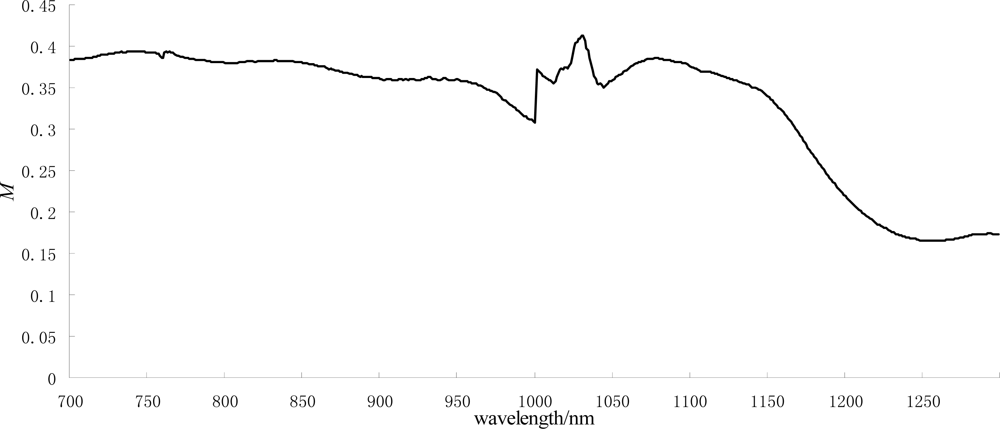
Figure 9.
Snow-covered areas of the Binggou watershed.

Figure 10.
Histogram of band 89.
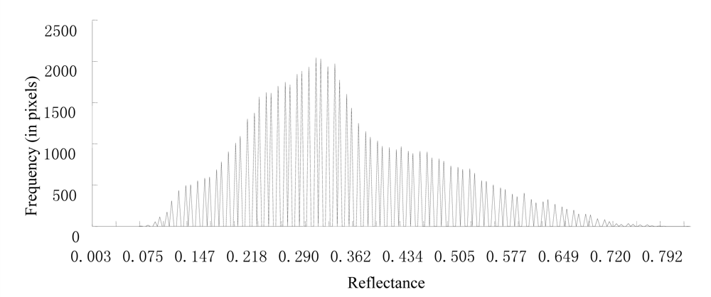
Figure 11.
The relationship between the snow grain size and reflectance at band 89.

Figure 12.
Distribution of the snow grain size estimated using the linear and exponential models. (a) Linear model, (b) Exponential model.
Figure 12.
Distribution of the snow grain size estimated using the linear and exponential models. (a) Linear model, (b) Exponential model.
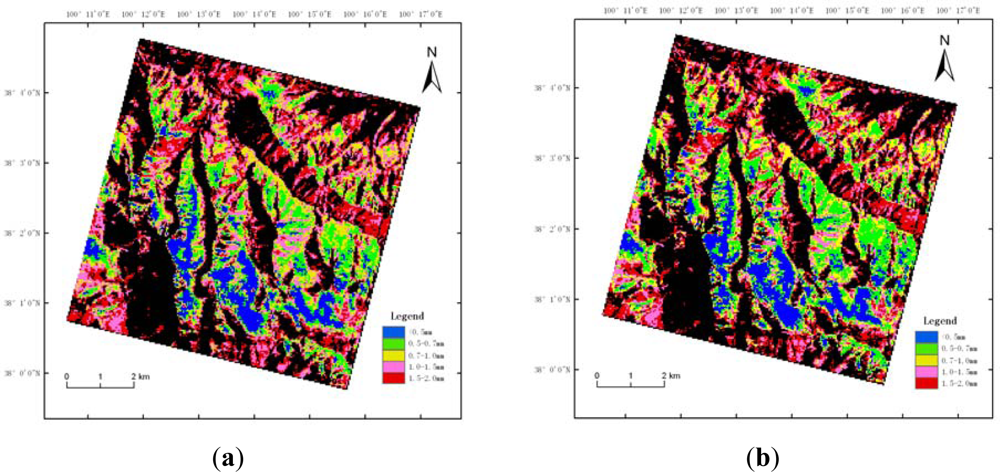
Figure 13.
The distribution of the wavelength location of absorption valleys.
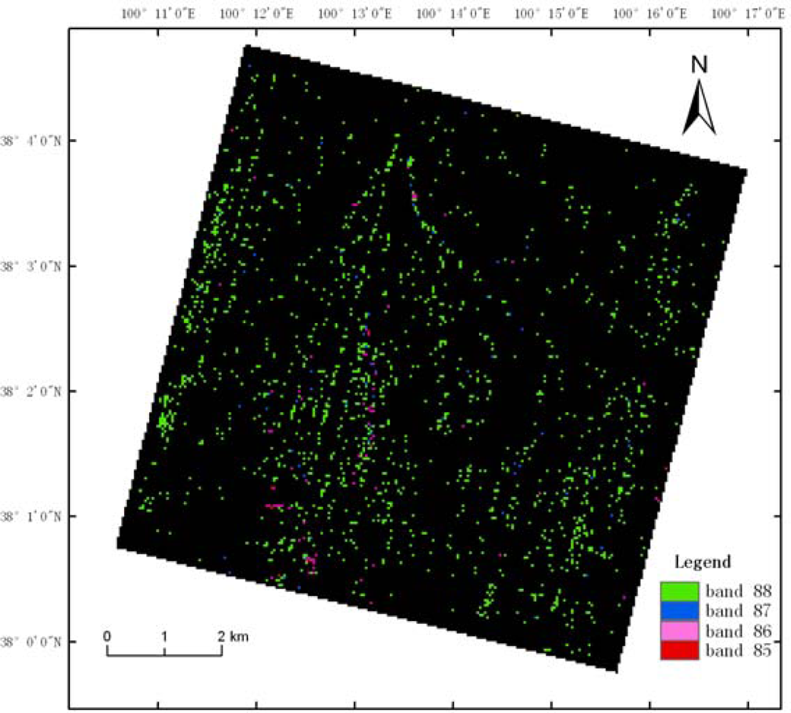
Figure 14.
New distribution of the snow grain size.

Figure 15.
Linear relationship between estimated and measured snow grain sizes.


| Measured Snow Grain Sizes | Estimated Snow Grain Sizes | Total | ||||
|---|---|---|---|---|---|---|
| <0.5 | 0.5–0.7 | 0.7–1.0 | 1.0–1.5 | 1.5–2.0 | ||
| <0.5 | 19 | 6 | 0 | 0 | 0 | 25 |
| 0.5–0.7 | 6 | 11 | 5 | 4 | 0 | 26 |
| 0.7–1.0 | 1 | 2 | 22 | 4 | 0 | 29 |
| 1.0–1.5 | 0 | 2 | 7 | 31 | 7 | 47 |
| 1.5–2.0 | 0 | 0 | 0 | 6 | 30 | 36 |
| Total | 26 | 21 | 34 | 45 | 37 | 163 |
| Total of diagonal | 113 | Kappa coefficient | 0.611 | |||
Share and Cite
MDPI and ACS Style
Zhao, S.; Jiang, T.; Wang, Z. Snow Grain-Size Estimation Using Hyperion Imagery in a Typical Area of the Heihe River Basin, China. Remote Sens. 2013, 5, 238-253. https://doi.org/10.3390/rs5010238
AMA Style
Zhao S, Jiang T, Wang Z. Snow Grain-Size Estimation Using Hyperion Imagery in a Typical Area of the Heihe River Basin, China. Remote Sensing. 2013; 5(1):238-253. https://doi.org/10.3390/rs5010238
Chicago/Turabian StyleZhao, Shuhe, Tenglong Jiang, and Zhaojun Wang. 2013. "Snow Grain-Size Estimation Using Hyperion Imagery in a Typical Area of the Heihe River Basin, China" Remote Sensing 5, no. 1: 238-253. https://doi.org/10.3390/rs5010238