Vegetation Index Differencing for Broad-Scale Assessment of Productivity Under Prolonged Drought and Sequential High Rainfall Conditions

1
Jornada Experimental Range, US Department of Agriculture, Agriculture Research Service, P.O. Box 30003 MSC3JER, Las Cruces, NM 88003, USA
2
Jornada Experimental Range, New Mexico State University, P.O. Box 30003 MSC3JER, Las Cruces, NM 88003, USA
*
Author to whom correspondence should be addressed.
Remote Sens. 2013, 5(1), 327-341; https://doi.org/10.3390/rs5010327
Submission received: 16 November 2012
/
Revised: 27 December 2012
/
Accepted: 6 January 2013
/
Published: 17 January 2013
Abstract
:Spatially-explicit depictions of plant productivity over large areas are critical to monitoring landscapes in highly heterogeneous arid ecosystems. Applying radiometric change detection techniques we sought to determine whether: (1) differences between pre- and post-growing season spectral vegetation index values effectively identify areas of significant change in vegetation; and (2) areas of significant change coincide with altered ecological states. We differenced NDVI values, standardized difference values to Z-scores to identify areas of significant increase and decrease in NDVI, and examined the ecological states associated with these areas. The vegetation index differencing method and translation of growing season NDVI to Z-scores permit examination of change over large areas and can be applied by non-experts. This method identified areas with potential for vegetation/ecological state transition and serves to guide field reconnaissance efforts that may ultimately inform land management decisions for millions of acres of federal lands.
1. Introduction
Spatially-explicit depictions of plant production that are derived in a consistent and repeatable manner are critical to monitoring landscapes in heterogeneous arid and semi-arid grassland and savanna ecosystems (hereafter “rangelands”). Change detection techniques applied to remotely sensed data provide opportunities to identify and characterize changes in land surface conditions to assist decision-making for land management and to focus field reconnaissance efforts.
Predictions for future climate are increasing temperatures and variability in the amount and timing of rainfall in the water-limited regions of the southwestern USA [1,2]. These changes in conjunction with increasing pressure on resources posed by a rapidly growing human population in this region necessitate effective, consistent, and data-driven tools to guide land management decisions and envision novel scenarios. The USA encompasses approximately 312 million hectares of rangelands, 43% of which is managed by the federal government [3]. The millions of hectares under federal jurisdiction pose a particular challenge to meeting the need for data-driven models that are linked to ecosystem function.
Understanding vegetation dynamics is central to the assessment of rangeland resources [4]. Over the last twenty years there has been a shift to using conceptual models that integrate non-linear vegetation dynamics. These models, known as state-and-transition models (STMs), encapsulate the notion that vegetation communities are present in multiple stable states, where the term “state” refers to the physical structure and set of ecological processes associated with a particular vegetation community. Transitions between states are catalyzed by both persistent environmental pressures such as drought or soil degradation and catastrophic disturbance [5]. STMs are constructed according to “ecological sites” [6,7]. Ecological sites are part of the Land Resource Hierarchy developed by the USDA-NRCS ( http://soils.usda.gov/survey/geography/hierarchy/) and are distinguished according to soil type, climate and geomorphic position. Central to ecological site classification is the potential of a place to support a given vegetation community and to exhibit specific processes that lead to transitions in vegetation composition and/or structure from the expected historic state [6].
State-and-transition models use various ecological site-specific terms to depict different states. We use the generalized nomenclature adopted by Steele et al.[8]. Historic state describes an historic unaltered vegetation community; an altered state describes a vegetation community that has undergone minor changes in ecosystem structure and governing ecological processes, but the soil profile remains largely intact. A degraded state describes a vegetation community that has undergone major changes in ecosystem structure and the ecological processes that govern transitions. Minor losses may be observed from the uppermost soil layer (A horizon). In many parts of the southwestern US, adverse changes in the vegetation structure that lead to degraded states are primarily associated with increases in woody cover and decreases in the cover of native perennial grasses to create shrub- or tree-dominated states. The most degraded state is the Bare-Annuals state, where there is widespread depletion of the A horizon and almost all vegetation has been removed except for annual pioneer species.
Establishing direct relationships between remotely-sensed data and ecological states or sites is extremely challenging in arid rangelands due to (i) the heterogeneity and sparseness of the vegetation and (ii) that fact that not all states exhibit distinct spectral signatures [8]. We suggest that radiometric change detection techniques can serve as an effective method to evaluate land surface changes in the context of vegetation dynamics (i.e., state changes) predicted by STMs and to identify locations to focus field monitoring efforts. This is achieved by integrating the change surface with available spatially-explicit ancillary data.
Vegetation index differencing (VID) using moderate spatial resolution Landsat Thematic Mapper (TM) imagery is one way to achieve consistent depictions of land surface change for its multi-decadal record and ground resolved distance. VID is a radiometric method for detecting change in pixel values between dates [9] and avoids issues associated with other change detection techniques [10,11]. We sought to broadly assess land surface conditions in actively managed rangeland landscapes that occur on the interface of the Chihuahuan and Sonoran Deserts in the southwestern USA by capitalizing on the readily available Landsat 5 Thematic Mapper image archive [12].
We examined changes between pre- and post-growing season Normalized Difference Vegetation Index (NDVI) [13] values to depict the change in photosynthetic biomass over the growing season. We selected imagery for a year following persistent below-average rainfall in the region (2003) and a year following two historically high rainfall years (2009; see Figure 1). We hypothesized that ecological states representing different degrees of degradation (i.e., Historic, Altered, Degraded) would respond differently to conditions of drought and abundant rainfall. We sought to answer the following questions: (1) What ecological states exhibit most positive and negative change in NDVI after periods of above- and below-average rainfall? and (2) What can we infer from the pattern of NDVI responses with respect to state-specific vegetation dynamics?
2. Methods
2.1. Study Site
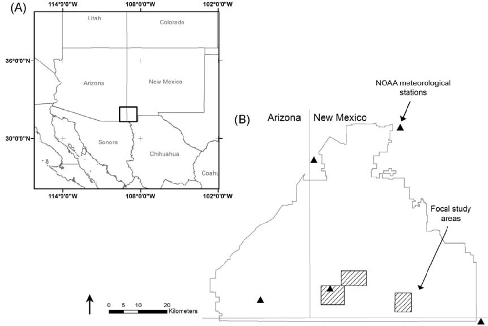
The Malpais Borderland Area (MBA) encompasses approximately 323,900 ha across southwestern New Mexico and southeastern Arizona along the border with Mexico (31.532 lat., −108.931 long.; Figure 2). Seventy-eight percent of the MBA is privately owned; the remaining 22% is under federal jurisdiction. The MBA occurs in the Basin and Range Province characterized by abrupt changes in elevation between valleys and basins interspersed among mountain ranges. Within the MBA, elevation ranges from 2,605 to 1,135 m and plant communities defined by Brown [14] include Chihuahuan Desert Scrub at the lowest elevations, Plains and Great Basin Grasslands along with Semi-desert Grasslands, Madrean Evergreen Woodlands, and Montane Conifer Forests at the highest elevations.
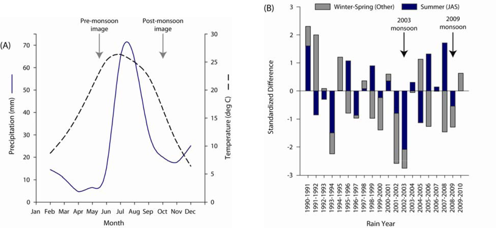
Precipitation in the region follows a unimodal distribution with 52% of annual rainfall occurring during summer months of July, August, and September (hereafter “monsoon,” Figure 1(A)). Long-term precipitation records from 1976 through 2010 were compiled for five NOAA meteorological stations that occur within two km of the MBA boundary (Figure 2). Average rainfall during monsoon months is 158.8 mm (Standard Deviation, SD = 55.3) with 146.6 mm (SD = 60.7) occurring in the remaining nine months. Average annual temperature peaks in July at 26.3 degrees C at the start of the monsoon season (Figure 1(B)).
Plant functional groups in this region exhibit marked differences in the timing of peak production, aboveground biomass, and canopy greenness. Deciduous (Prosopis and Quercus spp.) and evergreen (Larrea tridentata and Juniperus spp.) shrubs and trees that follow the C3 metabolic pathway leaf out and achieve well-developed canopies in the spring prior to the onset of monsoon precipitation in July. In contrast, co-occurring perennial grasses following the C4 metabolic pathway develop green canopies in late summer in response to the monsoon rainfall. Annual grasses and forbs may flourish in either spring or winter. The abundance of perennial grasses and annual grasses and forbs are informative criteria to distinguish the relative degree of degradation that defines ecological states. To facilitate ecological interpretation, we capitalized on phenological differences to examine a spring image prior to the monsoon rains and a late summer image (gray arrows in Figure 1(A)) for one year following prolonged below-average rainfall 2003, and one year following two years with record high rainfall during the monsoon months 2009. Four of the five years preceding 2003 exhibited below average rainfall with the two years prior under extreme drought (standardized difference values less than −2, Figure 1(B)). 2006 and 2008 were record high rainfall monsoon years.
2.2. Vegetation Index Differencing
Four Landsat 5 TM images were obtained from the Landsat Archive administered by the US Geological Survey [12] to capture spring and late summer conditions for 2003 and 2009. We selected images with <10% cloud cover and attempted to choose anniversary dates to avoid issues associated with differences in sun angle and shadow contributions to radiance emitted from surface. TM images selected for 2003 were acquired 1 May (DOY = 121) and 24 October (DOY = 297); 2009 images were acquired 17 May (DOY = 137) and 22 September (DOY = 265).
We corrected the effects of atmosphere and sun angle with the COST method using dark object subtraction and sun angle (tau) [15]. The lack of discernible invariant features (i.e., major roads, large water bodies) in the imagery precluded our ability to perform a radiometric normalization on the Landsat TM data. Normalized Difference Vegetation Index (NDVI) [13] data were derived using reflectance for each image. On a pixel-by-pixel basis, NDVI values in the spring image were subtracted from the late summer image to yield vegetation index difference (VID) images representing the change in NDVI over the growing season in the dry 2003 and wet 2009 rain years.
2.3. Change Assessment
2.3.1. Z-Score Calculation
Differences in 2003 and 2009 growing season NDVI (summer–spring; VID) were standardized to yield Z-scores to identify pixels of at the low and high ends of the tails of the distribution [16]. Standardized values for 2003 and 2009 represent anomalies of high and low growing season NDVI relative to the mean VID value for all pixels in the Malpais Borderlands study area (MBA). We assume that VID anomalies reflect plant community responses to extreme high and low growing season rainfall and that differences due to soils are accounted for by ecological sites. For 2003 and 2009 growing seasons, the Z-score for each ij pixel was calculated by subtracting the global mean VID based on values for all pixels in the MBA; this difference was then divided by the standard deviation (σ) for the global mean. Calculations for the 2003 NDVI difference values were made as specified in Equation (1):
Statistical inference using Z-scores is based on the assumption that values are normally distributed. To evaluate this assumption, we randomly sampled 2,000 pixels from the 2003 and 2009 growing season Z-score images and used a student’s t-test to determine whether the mean Z-scores are centered on zero. The 2003 growing season Z-scores were normally distributed (t = −0.63, p = 0.528) while the 2009 Z-scores were skewed to the right with a modest number of large patches (t = 6.59, p < 0.001). To demonstrate the utility of this approach to identify area of change in the tails of the distribution, we used −1.96 and 1.96 to identify the top and bottom 2.5% of the distribution based on a standard normal. Use of 1.96 as the threshold for positive change for the 2009 data that included 14 patches >100 ha in the right tail of the distribution captured greater than the top 2.5% of the distribution. In application, the threshold values can be modified to suit the mapping objectives.
2.3.2. Minimum Mapping Unit and Selection of Focal Areas
We reclassified the 2003 and 2009 Z-score images to generate contiguous patches with VID values in the tails of the distribution (positive, greater than 1.96 or negative, less than −1.96). The reclassified Z-score images were then filtered to dissolve patches that were smaller than the minimum mapping unit relevant for land management decision-making. The minimum mapping unit for this analysis was defined in conjunction with Natural Resource Conservation Service (NRCS) soil scientists to coincide with the 16.2 ha (or 40 acre) minimum size for soil inclusions. Patches were identified on the basis of four neighboring pixels; patches with less than 180 Landsat pixels were dissolved. The minimum mapping unit can be adjusted to represent the appropriate spatial scale for other applications. To represent the spatial arrangement of patches under-going extreme changes in NDVI over the growing season, we derived patch size distributions for all 2003 and 2009 patches representing anomalous increases or decreases in NDVI.
We selected three areas (hereafter, “focal areas”) that encompassed contiguous patches of pixels that signified positive anomalies (>1.96) or negative anomalies (<−1.96) in the 2003 and 2009 VID images. The three focal areas were 3,177, 3,907, and 4,358 ha in size, respectively and constitute the spatial extent for which ecological sites were mapped (hatched polygons, Figure 2(B)).
2.4. Ecological Sites and State Mapping
Within the MBA study area, ecological sites may be grouped according to the presence and amount of woody cover in the Historic state [8]. Two types of ecological sites occur in the focal areas: Type 1 Ecological sites with little woody cover in the Historic state and Type 2 Ecological sites with substantial woody cover within a grassland matrix in the Historic state. Henceforth, we refer to Type 1 Ecological sites as those with low to no woody cover component in the Historic state and Type 2 having a larger woody cover component in the Historic state (See Table 1).
Existing ecological site data are not mapped at a spatial resolution commensurate with plant community dynamics. To yield ecological state data of the appropriate scale, we created vector maps of ecological states across the three focal areas in accordance with the method and generalized state classes developed by Steele et al. [8]. This method involves photo-interpretation of fine spatial resolution aerial photography (in this case, National Agricultural Imagery Program (NAIP) 1 m imagery that was acquired in July 2009) and hand-editing of ecological site vector data, derived from Natural Resource Conservation Service Soil Survey Geographic database (SSURGO) soil map unit components of the National Cooperative Soil Survey [6].
We summarized VID results in the context of ecological states within Type 1 and Type 2 ecological sites based on state maps generated for the three focal areas. Percentages for each ecological site/state combination were calculated as the ratio of patch area for a given year and change (i.e., increase or decrease) and the total area for that ecological/state in the three focal areas (see Table 2). To represent significant changes in growing season NDVI in relation to the potential area that could undergo change, we express significant changes in NDVI in a given state as a function of the total area of that state (ΔAS/AS; Table 2). Significant changes are defined as those that occur in the tails of the z-score distribution with values greater than 1.96 or less than −1.96. We focus our interpretation on growing season anomalies on Type 1 ecological site because of the management emphasis placed on these ecological sites that are susceptible to woody plant encroachment [8].
3. Results
3.1. Patch Size Distributions for Positive and Negative Growing Season Anomalies
Over the 2003 growing season 5,178 ha (or 1.6% of the MBA study area) experienced significant decreases in NDVI. The majority of patches experiencing decreases in 2003 NDVI were small with 68 patches ranging from 10 to 20 ha in size while only two patches were greater than 100 ha; the maximum patch size was 300 ha. The 2009 growing season was characterized by increases in NDVI over 16,144 ha (or 5.0% of the study area). The number and size of patches of significant increase in 2009 were high. There were 100 patches between 10 and 20 ha in size and 14 patches greater than 100 ha; maximum patch size was 3,666 ha.
3.2. Ecological State Responses
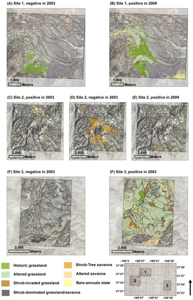
Ecological state responses were characterized for three focal areas covering 11,442 ha (Figure 2(B)). The widespread reductions in 2003 growing season NDVI occurred more commonly on Type 2 (i.e., Hills) ecological sites in 18.8% of the areas classified as Shrub-tree savanna state and 15.6% of the Shrub-dominated savanna state (Table 2). The 171.8 ha extent of Type 1 ecological sites that showed significant decreases in NDVI was dominated by response of Historic grassland state on the Clay Loam Upland ecological site (Figure 3(A)). Areas with increasing NDVI over the 2003 growing season were small (i.e., 81.3 ha) and dominated by Bare-Annuals (5.4%) and Shrub-invaded grassland (5.0%) ecological states (Figure 3(C)).
The broad-scale pattern of increases in NDVI over the 2009 growing season was consistent within the focal areas; there were no cases of 2009 decreases in NDVI in the focal areas. Increases in NDVI occurred in most ecological states, but with a 10-fold greater distribution on Type 1 ecological sites (2,936.2 ha or 45% of the area of Type 1 sites, Figure 3(G)) than occurred on Type 2 ecological sites (246.6 ha or 5% of the area of Type 2 sites, Figure 3(E)). Of the Type 1 ecological sites experiencing a significant increase in growing season NDVI, most changes occurred on the Altered grassland state (4,111.6 ha and 54.9% of Altered grasslands; Table 2, Figure 3(G)). The second largest increases occurred on the Historic grassland state (1,427.0 ha and 24.9% of Historic grasslands; Table 2, Figure 3(B,G)).
We highlight three examples of how changes in NDVI can be interpreted with respect to the vegetation dynamics conceptualized in STMs. We focus on Historic and Altered grasslands and Bare-Annuals states on Type 1 Ecological sites with a low woody cover component in the Historic state because of their susceptibility to woody plant encroachment.
3.2.1. Historic Grassland and Altered Grassland: Decrease of NDVI in 2003
Clay Loam Upland ecological sites in Historic and Altered grassland states exhibited significant decreases in growing season NDVI in 2003 following multiple dry years (e.g., Figure 3(A)). This decrease in NDVI over the growing season indicates that cool season plants which were photosynthetically active prior to the onset of monsoon rains (i.e., March–April) became increasingly senescent. Under prolonged dry conditions without sufficient moisture, there was little to no growing season production of photosynthetic biomass by ecologically important warm season grasses (e.g., Bouteloua sp.). Loss of perennial grass species is a precursor of a transition to an alternative ecological state [6,7], therefore negative growing season anomalies in NDVI for areas mapped as Historic or Altered grassland states would be a high priority for field assessment and survey.
3.2.2. Historic Grassland and Altered Grassland: Increase of NDVI in 2009
The significant increase in NDVI over areas in Historic grassland states in 2009 suggests that the stability of that ecological state is maintained or even improved; this increase in production could be driven by perennial grasses or annual species. Annual species are usually indicative of disturbance, but in some Historic grasslands such as those located on Clay Loam Upland Ecological sites, perennial grasses (Bouteloua sp. and Hilaria belangeri) are subdominant to native annual forbs such as Heliomeris longifolia var. annua[18]. Therefore, where Heliomeris is dominant, positive NDVI anomalies can be attributed to increased production by annual forb species, thus highlighting the value added to interpretations of change detection outputs by using Ecological site descriptions as a source of ancillary data.
In the Altered grassland state, native perennial grass species are less abundant, so increases in NDVI are more likely to portend a transition to an alternative less desirable state, such as the Exotic-invaded state. Over Clay Loam Upland sites in the MBA, Bothriochloa ischaemum, Eragrostis curvala and Eragrostis lehmanniana are known invasive species that are common in Exotic-invaded ecological states. Invasive plant species reduce biodiversity, displace desirable native species, alter disturbance (e.g., fire) regimes, and decrease productivity [19]. Mitigating the transition to an Exotic-invaded ecological state is of paramount importance to rangeland resource managers; field reconnaissance efforts would be greatly enhanced by spatially-explicit depictions of candidate sites.
3.2.3. Bare-Annuals: Increase of NDVI in 2003 and 2009
Increases in growing season NDVI are not necessarily associated with improved ecological states. Table 2 indicates that 5.4% of the Bare-Annuals (degraded) state in Type 1 Ecological sites represented positive NDVI anomalies in the 2003 drought year. In 2009, 33% of the area occupied by the Bare-Annuals state experienced significant increases in NDVI. In both cases of rainfall extremes, the positive NDVI anomalies occurred primarily on Loamy Bottom ecological sites. The 2003 significant increase can be attributed to the fact that these ecological sites are situated in topographic lows and are characterized by loamy soils with high water retention properties. Additionally, Loamy Bottom ecological sites often experience repeated disturbance associated with livestock activity (i.e., trampling and grazing of perennial grass species) because these sites commonly contain water tanks for livestock use. The Loamy Bottom Ecological Site Description [20] states that annual composite forbs that are typical of disturbed areas (e.g., Ambrosia psilostachya, Xanthocephalum gymnospermoides, Heliomeris longifolia var. annua, and other Asteraceae species) produce abundant photosynthetic biomass in wet seasons. Further, introduced grasses (Cynodon dactylon and Sorghum halepense) are known invasive species on Loamy Bottom ecological sites that also produce substantial biomass under conditions of sufficient moisture.
4. Discussion
Broad-scale monitoring of land surface conditions is a pressing need in many parts of the world as the demand for multiple uses intensifies. Remote sensing change detection provides an opportunity to evaluate and identify areas of change and assist in natural resource problem solving [21,22]. We used a multi-scale approach that integrating ecological state mapping using fine-resolution aerial photography with vegetation index differencing using moderate resolution satellite imagery to greatly enhance our interpretation of growing season responses to high and low rainfall. Moreover, interpretations of NDVI anomalies were informed by vegetation dynamics derived from state-and-transition models in an effort to facilitate ecosystem inventory and monitoring efforts.
While we can make inferences regarding NDVI changes using knowledge of vegetation dynamics in this region, this method must be developed further and correlated with field observations to verify our inferences. A traditional accuracy assessment was beyond the scope of this initial study. This is primarily because we lack ground data suitable for determining the degree of change in vegetation indicated by VID over such an expansive area of which much is difficult to access. Yet, future efforts are planned that will incorporate field visits to areas that demonstrated dynamic responses to drought and periods of high rainfall. The effort will incorporate on-the-ground data collection with on-going analysis of fine spatial resolution imagery image analysis to refine and inform the ecological state mapping process. The classification of ecological sites using fine spatial resolution imagery is a developing field that is most successfully accomplished with iterative refinement and development as field data are compiled [8]. We uphold the integrity of the ecological state maps generated in this study with expert knowledge and experience in interpreting vegetation patterns and associations with geomorphology discernible on the digital ortho-quarter quadrangle imagery; however, we acknowledge that the mapping of ecological state polygons represents a source of uncertainty. Where this expert knowledge is not available, VID interpretations could still be informed by readily-available ecological site polygons.
We present a case study to demonstrate how a multi-scale approach to change detection can effectively focus field reconnaissance efforts that in itself provides insight where field data are presently lacking. Further development can be greatly enhanced by incorporating longer time series such as Landsat data available through the Web-enabled Landsat Data (WELD) project [23].
We contend that even in the absence of field data or expert knowledge, the use of VID is valuable for prioritizing sites for field visits. Vegetation communities occurring in altered states have been shown to respond well to management intervention whereas a vegetation community in a highly degraded state is often beyond economical means of intervention. We recommend that locations where the vegetation communities are in historic or altered states and which appear as growing season NDVI anomalies (positive or negative) should be prioritized for field visits over locations showing less significant changes in NDVI. In this manner, spatially-explicit depictions of areas with potential for vegetation/ecological state transition would greatly enhance the effectiveness of field and management efforts across millions of acres of federal lands.
All remote sensing protocols designed to provide data needed for decision-making have strengths, weaknesses, and situations for which they function optimally. That the 2009 growing season NDVI VID values were not normally distributed does not compromise our ability to identify areas in the tails of the distribution to identify patterns and guide field efforts for broad-scale landscape monitoring. When research objectives or management needs require multiple depictions of land surface condition (either multiple dates or multiple sites at one time), growing season NDVI values must be standardized. If emphasis is placed on a mapping effort for a site at one point in time, the user could alternatively rank the VID values and choose those at the upper and lower ends of the distribution. This modification and/or non-parametric techniques could be used to avoid violating assumptions associated with normally distributed data.
Coppin et al.[24] and Singh [11] provide an effective treatment of logistical considerations as well as advantages and disadvantages of different change detection methods. The use of imagery collected at different spatial resolutions and the combination of manual (ecological state mapping) and automated (NDVI difference images) remote sensing methods provided an intuitive data product. This application of vegetation index differencing (VID) combines two benefits noted by Coppin et al.[24]; first, vegetation indices are more closely related to land surface changes than individual image bands, and second, VID is capable of detecting both abrupt and progressive changes in the land surface. The latter point is of tremendous benefit to those seeking to identify indicators that portend ecological state transitions. In addition, the direct use of radiometric data (i.e., spectral vegetation indices) and translation to growing season change in NDVI circumvents image classification errors associated with multi-date comparisons, or other post-processing and did not rely on robust relationships between NDVI and biophysical parameters, of which a notable lack exists in drylands. Lastly, there is flexibility in this approach in both the selection of the appropriate Z-score threshold to define “high” and “low” responses and the scale of observation, i.e., minimum patch size. Both refinements for thresholds and patch size should reflect the specificity and focal scale required to achieve the management or research objective [21]. The ability to modify these factors in a decision-making framework is highly valued by land managers [25].
There are research applications for which remotely sensed imagery assist, but do not fulfill decision-making needs and requirements [21] and the strengths and limitations should be duly noted. Land managers and decision-makers seek remote sensing tools that provide products relevant to and consistent with STM concepts [6,8,26]. This is a compelling challenge from two perspectives. The remote sensing community is needed to augment the knowledge regarding the accuracy and suitability of the full suite of change detection algorithms not presented here, e.g., [11,24,27] to promote understanding of which techniques are best suited for different research applications. Land managers and their technical collaborators are challenged to identify existing indicators or modifications thereof that are commensurate with products derived from remotely sensed data [25]. Only with contributions from both communities and effective dialogue between them will the full potential of remote sensing for natural resource management decision-making be realized.
5. Conclusions
The ability to quantitatively evaluate large tracts of land in a consistent manner using readily available moderate resolution satellite data is a highly valuable tool for land resource managers [22]. We used a multi-scale approach that integrates ecological state mapping using fine-resolution aerial photography with vegetation index differencing using moderate resolution satellite imagery to enhance our interpretation of growing season responses to high and persistent low rainfall. The approach is built upon automated and manual image analysis techniques, holds potential to identify those areas susceptible to degradation and possible candidates for management intervention, and can effectively prioritize sites for assessment and monitoring.
Acknowledgments
We thank Jason Karl for providing helpful comments on the manuscript and acknowledge the notable contribution of the US Geological Survey for providing free access to the Landsat data archive.
References
- Overpeck, J.; Udall, B. Dry times ahead. Science 2010, 328, 1642–1643. [Google Scholar]
- Woodhouse, C.A.; Overpeck, J.T. 2000 years of drought variability in the central United States. Bull. Amer. Meteorol. Soc 1998, 79, 2693–2714. [Google Scholar]
- Joyce, L.A. An Analysis of the Range Forage Situation in the United States: 1989–2040; General Technical Report RM-180; US Department of Agriculture, Forest Service, Rocky Mountain Range and Forest Experiment Station: Fort Collins, CO, USA, 1989; p. 90. [Google Scholar]
- Briske, D.D.; Fuhlendorf, S.D.; Smeins, F.E. State-and-transition models, thresholds, and rangeland health: A synthesis of ecological concepts and perspectives. Rangel. Ecol. Manage 2005, 58, 1–10. [Google Scholar]
- Bestelmeyer, B.T.; Brown, J.R.; Havstad, K.M.; Alexander, R.; Chavez, G.; Herrick, J.E. Development and use of state-and-transition models for rangelands. J. Range Manage 2003, 56, 114–126. [Google Scholar]
- Bestelmeyer, B.T.; Tugel, A.J.; Peacock, G.L.; Robinett, D.G.; Shaver, P.L.; Brown, J.R.; Herrick, J.E.; Sanchez, H.; Havstad, K.M. State-and-transition models for heterogeneous landscapes: A strategy for development and application. Rangel. Ecol. Manage 2009, 62, 1–15. [Google Scholar]
- Briske, D.D.; Bestelmeyer, B.T.; Stringham, T.K.; Shaver, P.L. Recommendations for development of resilience-based state-and-transition models. Rangel. Ecol. Manage 2008, 61, 359–367. [Google Scholar]
- Steele, C.M.; Bestelmeyer, B.T.; Burkett, L.M.; Smith, P.L.; Yanoff, S. Spatially explicit representation of state-and-transition models. Rangel. Ecol. Manage 2012, 65, 213–222. [Google Scholar]
- Nelson, R.F. Detecting forest canopy change due to insect activity using Landsat MSS. Photogramm. Eng. Remote Sensing 1983, 49, 1303–1314. [Google Scholar]
- Alphan, H. Comparing the utility of image algebra operations for characterizing landscape changes: The case of the Mediterranean coast. J. Environ. Manage 2011, 92, 2961–2971. [Google Scholar]
- Singh, A. Review article: Digital change detection techniques using remotely-sensed data. Int. J. Remote Sens 1989, 10, 989–1003. [Google Scholar]
- Woodcock, C.E.; Allen, R.; Anderson, M.; Belward, A.; Bindschadler, R.; Cohen, W.; Gao, F.; Goward, S.N.; Helder, D.; Helmer, E.; et al. Free access to Landsat imagery. Science 2008, 320, 1011–1011. [Google Scholar]
- Tucker, C.J. Red and photographic infrared linear combinations for monitoring vegetation. Remote Sens. Environ 1979, 8, 127–150. [Google Scholar]
- Brown, D.E. Biotic Communities: Southwestern United States and Northwestern Mexico; University of Utah Press: Salt Lake City, UT, USA, 1994; p. 342. [Google Scholar]
- Chavez, P.S., Jr. Image-based atmospheric corrections--revisited and improved. Photogramm. Eng. Remote Sensing 1996, 62, 1025–1036. [Google Scholar]
- Peters, A.J.; Walter-Shea, E.A.; Ji, L.; Vina, A.; Hayes, M.; Svoboda, M.D. Drought monitoring with NDVI-based standardized vegetation index. Photogramm. Eng. Remote Sensing 2002, 68, 71–75. [Google Scholar]
- National Resources Conservation Service. Land Resource Regions and Major Land Resource Areas of the United States, the Caribbean, and the Pacific Basin; USDA Arigcultural Handbook 296; National Resource Conservation Service, USDA: Washington, DC, USA, 2006; p. 682. [Google Scholar]
- USDA-NRCS. Ecological Site Description: Clay Loam Upland (R041XA109AZ); National Resource Conservation Service, USDA: Washington, DC, USA, 2005. [Google Scholar]
- Sheley, R.L.; James, J.J.; Rinella, M.J.; Bluemthal, D.; di Tomaso, J.M. Invasive Plant Management on Anticipated Conservation Benefits: A Scientific Assessment. In Conservation Benefits of Rangeland Practices—Assessment, Recommendations, and Knowledge Gaps; Briske, D.D., Ed.; US Department of Agriculture Natural Resource Conservation Service: Washington, DC, USA, 2011. [Google Scholar]
- USDA-NRCS. Ecological Site Description: Loamy Bottom (RO41XA114AZ); National Resource Conservation Service, USDA: Washington, DC, USA, 2005. [Google Scholar]
- Ludwig, J.A.; Bastin, G.N.; Wallace, J.F.; McVicar, T.R. Assessing landscape health by scaling with remote sensing: When is it not enough? Landscape Ecol 2007, 22, 163–169. [Google Scholar]
- Forbis, T.A.; Provencher, L.; Turner, L.; Medlyn, G.; Thompson, J.; Jones, G. A method for landscape-scale vegetation assessment: Application to great basin rangeland ecosystems. Rangel. Ecol. Manage 2007, 60, 209–217. [Google Scholar]
- Roy, D.P.; Ju, J.C.; Kline, K.; Scaramuzza, P.L.; Kovalskyy, V.; Hansen, M.; Loveland, T.R.; Vermote, E.; Zhang, C.S. Web-enabled Landsat Data (WELD): Landsat ETM plus composited mosaics of the conterminous United States. Remote Sens. Environ 2010, 114, 35–49. [Google Scholar]
- Coppin, P.; Jonckheere, I.; Nackaerts, K.; Muys, B.; Lambin, E. Digital change detection methods in ecosystem monitoring: A review. Int. J. Remote Sens 2004, 25, 1565–1596. [Google Scholar]
- Karl, J.W.; Herrick, J.E.; Browning, D.M. A vision for rangeland management based on best available knowledge and information. Rangel. Ecol. Manage 2012, 65, 638–646. [Google Scholar]
- Briske, D.D.; Fuhlendorf, S.D.; Smeins, F.E. A unified framework for assessment and application of ecological thresholds. Rangel. Ecol. Manage 2006, 59, 225–236. [Google Scholar]
- Wilson, J.R.J.; Blackmon, C.; Spann, G.W. Land use change detection using Landsat data. Remote Sens. Earth Resour 1977, 5, 79–91. [Google Scholar]
Figure 1.
Climatic patterns for the Malpais Borderland Area calculated using data from five NOAA meteorological stations from 1990 through 2010. Panel (A) depicts the mean monthly precipitation (solid blue line) and temperature (black dotted line); gray arrows indicate the temporal range of Landsat TM 5 imagery used in this study. Panel (B) is a standardized difference from long-term average calculated seasonally based on standard water year (October through September). In this region, the growing season (July, August, and September; Panel (A)) occurs at the end of the water year.

Figure 2.
(A) Location of 324,000 ha Malpais Borderland study area in southwestern USA. (B) Meteorological stations within 2 km of the study site and three focal areas for which ecological states were mapped (hatched polygons) are presented in Panel (B).
Figure 2.
(A) Location of 324,000 ha Malpais Borderland study area in southwestern USA. (B) Meteorological stations within 2 km of the study site and three focal areas for which ecological states were mapped (hatched polygons) are presented in Panel (B).

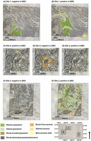
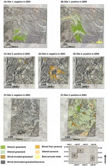
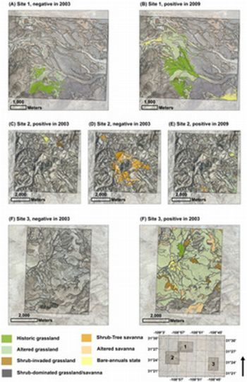
Figure 3.
Distribution of ecological states (gray outlines) within areas demonstrating NDVI growing season anomalies (A) Site 1, negative change in 2003; (B) Site 1, positive change 2009; (C) Site 2, positive change in 2003; (D) Site 2, negative change 2003; (E) Site 2, positive change, 2009; (F) Site 3, negative change in 2003; (G) Site 3, positive change 2009. Gray outlines depict ecological state boundaries prior to grouping.


Table 1.
Ecological site and state designations within the Malpais Borderlands Area (MBA) study area. Ecological sites came from the Natural Resource Conservation Service (NRCS) Soil Survey Geographic database (SSURGO) ecological site information [17]. Within these Major Land Resource Areas, ecological sites may be grouped according to the presence and amount of woody cover in the Historic state; Type 1 sites have little to no woody cover and Type 2 sites have a woody cover component in the Historic state [8].
| Type 1 Ecological Sites | Condition | Ecological State | Area (AS, [Ha]) | % of MBA |
| Clay Hills, Clay Loam Upland, Draw, Gravelly Slopes, Hills (41.1&), Loamy, Loamy Bottom, Loamy Upland | Reference | Historic grassland | 1,426.97 | 12.48 |
| Altered | Altered grassland | 4,111.91 | 35.96 | |
| Altered | Shrub-invaded grassland | 441.91 | 3.86 | |
| Degraded | Shrub-dominated grassland | 10.73 | 0.09 | |
| Degraded | Bare-Annuals | 505.69 | 4.42 | |
| Total | 6,497.21 | 56.82 | ||
| Type 2 Ecological sites | Condition | Ecological state | Area (AS, [Ha]) | % of MBA |
| Hills (42.2*) | Reference | Shrub-Tree Savanna | 1,716.83 | 15.01 |
| Altered | Altered Savanna | 3,007.03 | 26.30 | |
| Degraded | Shrub-dominated Savanna | 213.54 | 1.87 | |
| Total | 4,937.40 | 43.18 | ||
&41.1 denotes MLRA 41, Common Resource Area 1;
*42.2 denotes MLRA 42, Common Resource Area 2.
Table 2.
Distribution of ecological sites and states representing growing season anomalies (i.e., growing season NDVI Z-score > 1.96 or < −1.96). Percentages are based on the extent of Ecological states within the three focal areas (hatched polygons in Figure 2). Type 1 and Type 2 Ecological sites were grouped according to the presence and amount of woody cover in the Historic state; Type 1 sites have little to no woody cover and Type 2 sites have a woody cover component in the Historic state [8]. There were no patches of negative change (i.e., areas of anomalous decrease in NDVI) in 2009 within the three focal areas.
| Negative Change 2003 | Ecological State | Area of Change (DAS [Ha]) | Total State Area (AS [Ha]) | % Age of Total State Area (DAS/AS) |
| Type 1 Ecological sites | ||||
| Clay Loam Upland, Gravelly Slopes, Hills (41.1), Loamy, Loamy Bottom | Historic grassland | 110.60 | 1,426.97 | 7.75 |
| Altered grassland | 51.11 | 4,111.58 | 1.24 | |
| Shrub-invaded grassland | 10.07 | 441.91 | 2.28 | |
| Bare-Annuals | 0.05 | 505.69 | 0.01 | |
| Total area changed (DA) | 171.84 | |||
| Type 2 Ecological sites | ||||
| Hills (42.2) | Shrub-Tree savanna | 323.03 | 1,716.83 | 18.82 |
| Altered Savanna | 169.12 | 3,007.03 | 5.62 | |
| Shrub-dominated Savanna | 33.42 | 213.54 | 15.65 | |
| Total area changed (DA) | 525.57 | |||
| Positive Change 2003 | Ecological State | Area of Change (DAS [Ha]) | Total State Area (AS [Ha]) | % Age of Total State Area (DAS/AS) |
| Type 1 Ecological sites | ||||
| Gravelly Slopes, Hills (41.1), Loamy Bottom | Altered grassland | 27.31 | 4,111.58 | 0.66 |
| Shrub-invaded grassland | 21.94 | 441.91 | 4.96 | |
| Bare-Annuals | 27.04 | 505.69 | 5.35 | |
| Total area changed (DA) | 76.29 | |||
| Type 2 Ecological sites | ||||
| Hills (42.2) | Shrub-Tree Savanna | 0.81 | 1,716.83 | 0.05 |
| Altered Savanna | 4.20 | 3,007.03 | 0.14 | |
| Total area changed (DA) | 5.01 | |||
| Positive Change 2009 | Ecological State | Area of Change (DAS [Ha]) | Total State Area (AS [Ha]) | % Age of Total State Area (DAS/AS) |
| Type 1 Ecological sites | ||||
| Clay Loam Upland, Draw, Gravelly Slopes, Hills (41.1), Loamy Bottom, Loamy Upland | Historic grassland | 355.68 | 1,426.97 | 24.93 |
| Altered grassland | 2,255.08 | 4,111.58 | 54.85 | |
| Shrub-invaded grassland | 146.29 | 441.91 | 33.11 | |
| Shrub-dominated grassland | 10.73 | 16.85 | 63.70 | |
| Bare-Annuals | 168.40 | 505.69 | 33.30 | |
| Total area changed (DA) | 2,936.18 | |||
| Type 2 Ecological sites | ||||
| Hills (42.2) | Shrub-Tree savanna | 16.97 | 1,716.83 | 0.99 |
| Altered Savanna | 173.69 | 3,007.03 | 5.78 | |
| Shrub-dominated Savanna | 55.91 | 213.54 | 26.18 | |
| Total area changed (DA) | 246.58 | |||
Share and Cite
MDPI and ACS Style
Browning, D.M.; Steele, C.M. Vegetation Index Differencing for Broad-Scale Assessment of Productivity Under Prolonged Drought and Sequential High Rainfall Conditions. Remote Sens. 2013, 5, 327-341. https://doi.org/10.3390/rs5010327
AMA Style
Browning DM, Steele CM. Vegetation Index Differencing for Broad-Scale Assessment of Productivity Under Prolonged Drought and Sequential High Rainfall Conditions. Remote Sensing. 2013; 5(1):327-341. https://doi.org/10.3390/rs5010327
Chicago/Turabian StyleBrowning, Dawn M., and Caitriana M. Steele. 2013. "Vegetation Index Differencing for Broad-Scale Assessment of Productivity Under Prolonged Drought and Sequential High Rainfall Conditions" Remote Sensing 5, no. 1: 327-341. https://doi.org/10.3390/rs5010327